the Creative Commons Attribution 4.0 License.
the Creative Commons Attribution 4.0 License.
 | 09 Aug 2021
Inhomogeneous precursor characteristics of rock with prefabricated cracks before fracture and its implication for earthquake monitoring
Andong Xu
Yonghong Zhao
Muhammad Irfan Ehsan
Jiaying Yang
Ru Liu
Earthquake precursors and earthquake monitoring are always important in the earthquake research field, even if there is still debate about the existence of earthquake precursors. However, it is extremely difficult to observe the seismogenic environment of earthquakes directly. Laboratory rupture experiment is a useful technique to simulate and gain an insight into the complex mechanisms of earthquakes. Five marble samples with prefabricated cracks are used for uniaxial loading experiments to investigate whether there is a precursory signal before rock fracture and to simulate the rupture process of strike-slip fault. The existence of a precursory signal is confirmed by the coefficient of variation (CV) results, from which we can see two patterns which are known as seismicity acceleration and quiescence before an earthquake. Moreover, these CV findings are applied to determine the locations of large deformation sampling points on the rock surface at different loading stages. Similar results are obtained when we consider actual seismicity at the northern end of the San Andreas Fault in California, which provides crucial evidence to prove the existence of precursor characteristics. In this case, three kinds of seismic monitoring models are designed to find out how to monitor these characteristics more effectively.
- Article
(13843 KB) - Full-text XML
-
Supplement
(1085 KB) - BibTeX
- EndNote


The issues of earthquake such as initiation, growing, and monitoring are difficult but attractive. Considerable efforts have been made to understand earthquake source mechanisms (Goff et al., 1987; Frohlich and Apperson, 1992; Frohlich, 2001; Kagan, 1991, 2005, 2013; Aldamegh et al., 2009; Butler, 2019). It is now generally believed that earthquakes are caused by a sudden release of accumulated energy, which induced a sudden failure of intact rock or sudden stick-slip motions on pre-existing faults. The essential factors that affect these sudden stick-slip motions depend on fault properties, but it is extremely difficult to directly measure these properties such as friction strength and stress state. Laboratory rock experiment is a useful approach to gain insights into rock and fault properties, including rate-and-state friction (Dieterich, 1979; Ruina, 1983; Rubin, 2008) and deformation under different conditions, such as in torsion or low temperature (Paterson and Olgaard, 2000; Beeler et al., 2007). Some of the other experiments which are known as laboratory earthquakes provide deep understanding of dynamic rupture processes, including supershear (Xia et al., 2004, 2005; Kammer et al., 2018) and fracture energy (Lockner et al., 1991; Kammer and McLaskey, 2019). However, this is still an unsolved problem, as Kammer and McLaskey (2019) said how these laboratory observations should be scaled to the sizes and rates of naturally occurring earthquake fault ruptures. We try to make a different type of analysis to link the laboratory observations with natural seismicity by comparing their similar characteristics.
More and more precursors before rock fracture have been observed under the progress of rock experiment in the laboratory. Brace et al. (1966) showed that the dense igneous rocks increase in volume before fracture. Under differential stress, rocks dilate before failure, which is caused by the development of new cracks within the rock. These observations led Nur (1972) to suggest that the ratio of (where Vp is the seismic P-wave velocity and Vs is the seismic S-wave velocity) should decrease if the rock becomes dilatant under stress and then increase again if water flows into the cracks from the surrounding regions. When a rock is stressed to failure, cracking on a microscopic scale occurs. These microcrack activities known as acoustic emission are considered a scale model of seismicity in the earth. There is a strong correlation between the amount of nonelastic strain and the number of acoustic emission events (Scholz, 1968). Some researchers find that as the rock approaches fracture, the acoustic emission rate increases (Scholz, 1968; Lockner and Byerlee, 1977), while others have discovered a decrease just before failure (Brady, 1975; Kahir, 1977). Acoustic emission has been used to predict rock bursts in deep mines in the late 1930s (Obert, 1977). In order to analyze the rock properties for understanding the natural dynamic rupture processes, characteristics and deformation of rock fracture have been observed with the development of the experimental technique, including the influence of crack size on the fracture behavior (Harlin and Willis, 1990), scaling and universality in rock fracture (Davidsen et al., 2007), and triggering processes in rock fracture (Davidsen et al., 2017). However, how these experimental results correspond to natural seismic observations is still less discussed, which may be essential for application of rock experiments and simulating actual earthquake. We attempt to make a comparison between laboratory consequences and natural findings to explore the possibility of this connection.
We introduce an attribute statistic called the coefficient of variation (CV) to quantify the deformation characteristics of rock fracture and to find the potential precursor that is useful for coupling laboratory experiments with natural earthquakes. We use five marble rock samples with prefabricated cracks to simulate the actual strike-slip fault such as the northern end of the San Andreas Fault (SAF) and to analyze the process of dynamic rupture during loading with the digital speckle correlation method (DSCM) (Peters and Ranson, 1982; Yamaguchi, 1981; Ma et al., 2004). By quantifying the deformation of rock fracture, the precursor characteristics have been identified. These features are used to determine the position of the sampling points with relatively large deformation, and we then detect their changes with the increase in load. We also study the distribution of epicenters in the seismic catalogue near the northern end of the SAF and try to compare the experimental results with it in order to investigate the common features between them. Finally, considering the actual situation, we design three different seismic monitoring models and compare their monitoring effects on precursors, hoping to provide some guidance for the earthquake monitoring work.
2.1 Digital speckle correlation method
The DSCM was proposed by Peters and Ranson (1982) and Yamaguchi (1981) in the early 1980s, respectively. The basic governing phenomena of the DSCM are to calculate the correlation coefficient between the source image and the target image, as shown in Fig. 1. We first co-register images of rock sample surfaces acquired before and after deformation based on a high-speed camera (about 3.74 fps s−1) and a speckle pattern. Then, we distribute image patches (with the size of 41-by-41 pixel squares in one patch) covering the rock sample surfaces (take “f” in the source image and “g” in the target image for example) and calculate pixel offsets using a certain correlation function (Ma et al., 2004). The difference (u,v) in pixel coordinates between “P” and “P′” is the displacement after deformation, and its derivative represents the strain.

The DSCM extracts the displacement and strain information from random speckle signals produced by artificial or natural texture. Dynamic measurement can be achieved by high-speed video recording or a high-speed photography system as the DSCM is the direct solving process of two recorded images. We use an artificial speckle and photography system (about 3.4 frames per second) to record the deformation images of the marble samples with prefabricated cracks during loading. By recording the images under different loads, the surface displacement and strain of the samples are worked out by the DSCM. For precision measurement, the pixel-level search is not enough, and the sub-pixel-level search should be completed by interpolation, iterative or fitting, which are introduced in Ma et al. (2004). The accuracy for displacement in our research is expected to be 0.01 pixels, and each pixel represents 0.04 mm.
2.2 Experiments with uniaxial loading
Five marble samples with prefabricated cracks are used in the experiments in order to discover and analyze the common rather than unique precursor characteristics before rupturing under loading. The five marble samples are all prepared as shown in Fig. 2a, and the precast cracks are used for simulating the actual strike-slip faults such as the northern end of the SAF. We analyze the dynamic rupture process during loading by the DSCM.
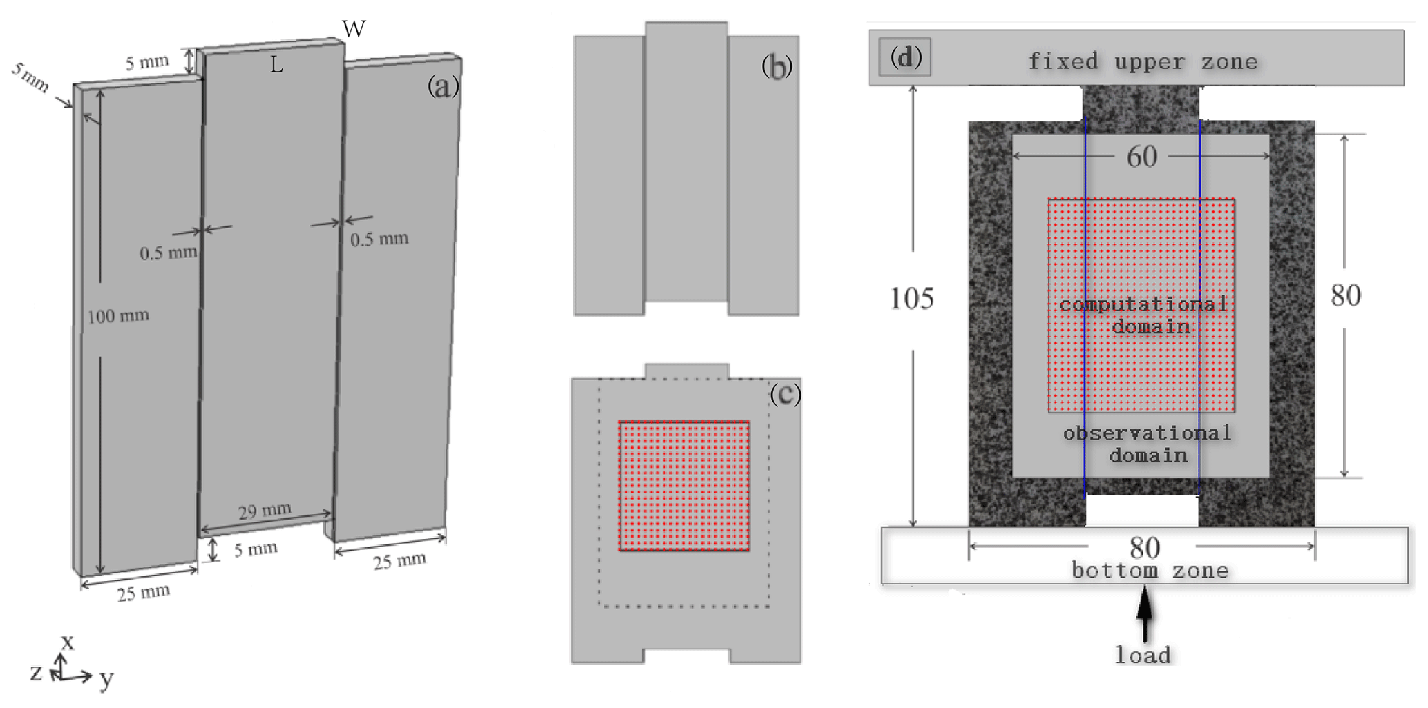
Figure 2Schematic diagram of the sample and experimental device. Three-dimensional shape of the sample. (a) The deep black lines indicate the prefabricated cracks. L is the length of the upper surface, while W is the width of it. The directions of three-dimensional coordinates are shown in the lower left corner. (b) Two-dimensional shape of the sample. (c) Two-dimensional shape of the sample. The area enclosed by the dash-line rectangle is the observational domain, and the solid-line rectangle is the computational domain. The red dots space 5 pixels apart from each other are the sampling points in the computational domain. (d) Experimental loading mode and observational and computational domain of the sample. There are random artificial speckle signals on the sample. The arrow indicates the direction of loading, and the two blue lines show the precast cracks. The gray zone represents the observational domain, and the area enclosed by the rectangle is the computational domain.
The size indicated in Fig. 2a is ideal, and there may be some deviation in the actual production of the samples. We spray speckles on the surface of these five marble samples to construct grayscale characteristics that can be used for the DSCM. Before the experiments, we measured the length and width of the upper surface of each sample since load would act on it (i.e., L and W in Fig. 2a). The detailed data of the five samples were listed in Table 1.
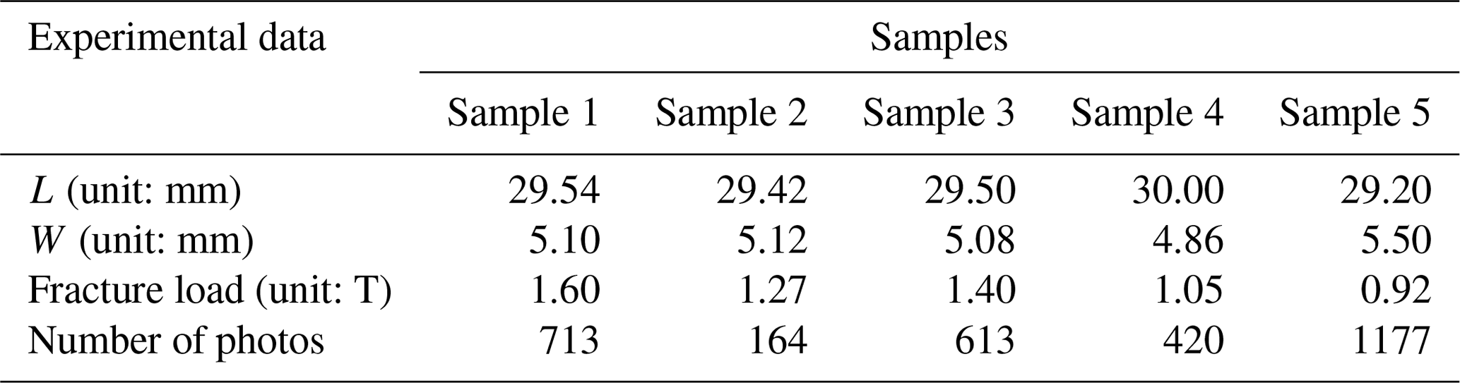
All of the experiments are performed in the same way on a uniaxial loading apparatus whose upper zone could be fixed as shown in Fig. 2d. The direction of loading was also shown in Fig. 2d, and the rate of load increase was artificially controlled. A photography system (about 3.4 frames per second) is used to film the entire process from initiation to destruction of the samples during loading. The number of photos we got for each sample during loading and the maximum load were listed in Table 1. We calculated all the photos using the DSCM in the case of the selected observation and computation domains shown in Fig. 2d.
2.3 Coefficient of variation
The CV, defined by a formula (Eq. 1), is a statistical relationship which is used to describe the dispersion degree of a set of data ().
where σ represents the standard deviation and μ is the mean value of the data set. The computation of σ is described in Eq. (2),
and the mathematical expression of μ is given in Eq. (3).
Kagan and Jackson (1991) used this statistic to describe the clustering of earthquake inter-occurrence time. Here, we applied the CV to describe the precursory characteristics of failure of the samples with prefabricated cracks, since the deformation degree of each part of the samples is intuitively different with the increase in load. In other words, we wanted to use this statistic to find out whether there is a significant signal before rupturing since the dispersion degree of the data fluctuates with loading. We have chosen the image of each sample in the initial state (i.e., without load) as the source image, and the third, fifth, seventh, and so on till the destruction image as the target images, which were all taken by the photography system. Various results can be obtained with the DSCM, including the displacement and strain of each sampling point in the computational region. Therefore, selecting the proper data to calculate the CV is the next crucial step.
Actually, the data we have recorded in real life, such as GPS data, crustal stress data, and other data, are all compared with a certain state rather than the initial state because we cannot know and record the initial state of a natural area. Thus, we proposed a so-called increment method to calculate our data to be consistent with the actual situation. Firstly, we obtained the displacement and strain of every moment during loading by selecting the initial state image as the source image and the later state images as target images. Then, the differential displacement and strain of each sampling point in the computational domain were acquired by subtracting the results of the previous moment from the results of the later moment, which is what we call increment. The displacement and strain of each sampling point obtained by this method constituted what we call differential displacement field and differential strain field. It is worth noting that we focus on the dispersion degree rather than the positive or negative characteristics of the data, so we calculated the CV after taking the absolute value of the increment. Except for the linear and shear strain, which we can obtain from the DSCM directly, we have also considered the maximum and minimum principal strains. Relationships for calculating these two strains are shown below.
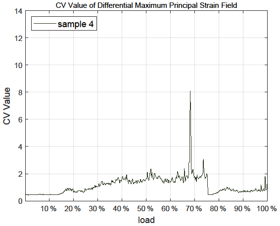
εx and u are linear strain and in parallel direction of the load; εy and v are linear strain and displacement perpendicular to load direction; εxy and γxy are shear strain in rock mechanics and engineering, respectively. The calculation steps of the corresponding differential maximum and minimum principal strain fields were consistent with the increment method. The CVs of all data above are calculated by using Eqs. (1)–(3). We put the CV of differential maximum principal strain for sample 4 here to analyze since its characteristics are clear (the others are in Fig. S1 in the Supplement). The similar images of the other samples are in the Appendices (Figs. A1–A4).
As can be seen from this image, the CV fluctuates with load and shows a significant jump at about the 70 % loading stage before rock fracture (100 % loading stage), which is what we call the precursory characteristic. This kind of precursor can appear when the CVs of proper physical quantities are monitored and calculated. As for the experimental results, we believe that the CV results obtained by calculating the differential strain field are better than those got from the differential displacement field, because the displacement is actually very sensitive to loading and the displacement of each sampling point is relatively large at the laboratory scale. In this case, the variation of the CV is not so obvious, which can be seen in the CV images of multiple samples (Figs. A1–A4). In contrast, the strain field can reflect the concentration of deformation, so it is useful for extracting the dispersion characteristics of the data and such precursory signals. Furthermore, the maximum principal strain is generated by the maximum principal stress, and the CV calculated by this strain has obvious precursor signals, such as the significant jump during 60 % to 80 % and a small jump near the 100 % loading stage shown in Fig. 3. Considering these two factors, we take the differential maximum principal strain as the monitoring signal of the earthquake monitoring models.
2.4 Compare the experimental results with the natural seismicity
The differential maximum principal strain is also used to distinguish the sampling points with large deformation, which contribute to the CV jump. It is not difficult to notice that the CV reaches 8 at around the 60 %–80 % loading stage in Fig. 3, so we have taken 8 as a judgement condition (which is also called the threshold) to find these large deformation points for sample 4. Here we still take the results of sample 4 for analysis. At every 10 % loading stage, the differential maximum principal strain of each sampling point is compared with the average differential maximum principal strain of all sampling points. If the differential maximum principal strain of a sampling point is 8 or more times larger than the average value of all sampling points, we will mark the position of this sampling point on the surface of sample 4 and try to display all the qualified sampling points at the same stage. It should be mentioned that the threshold of different samples is not the same according to the CVs of samples. Therefore, we take 4 as a threshold for sample 1, 3 for samples 2 and 3, and 4 for sample 5. We show the results of sample 4 at the 100 % loading stage in Fig. 4 (the results at the other loading stage are in Fig. S2 in the Supplement), and the other samples' results are shown in Appendix B (Figs. B1–B4).
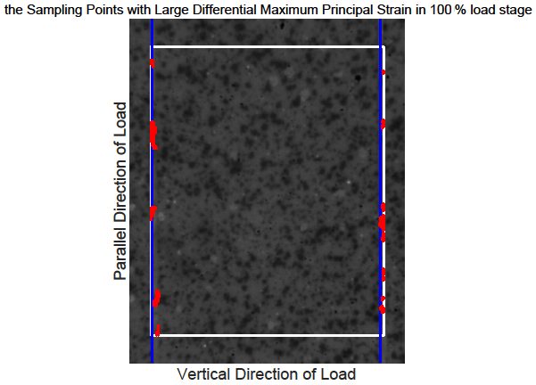
Figure 4The position of the sampling points with large differential maximum principal strain for sample 4. The blue lines indicate the prefabricated cracks. Each figure shows the observational area of sample 4 in the experiments. The area enclosed by the white rectangle is the calculation domain, and its size is constant in different loading stages. The red points represent the sampling points with large differential maximum principal strain that satisfy the judgment condition at the 100 % load stage.
Figure S2 shows that some sampling points with large differential maximum principal strain that satisfy the judgement condition began to appear at the 30 % loading stage, which corresponds to the phenomenon that the CV starts to rise in Fig. 3. Then the position of such sampling points changes with the increase in load, and the deformation becomes larger and larger. According to Fig. 3, the CV reaches the maximum level at about 70 % fracture load and then enters the quiet period until sample 4 is broken when the load is 100 %. When sample 4 approaches fracture, the sampling points with large deformation are concentrated near the precast crack. The consequences of the other samples also show this concentration phenomenon, which leads us to have an interest in investigating the location of earthquakes near strike-slip faults. In particular, we want to know how the location of small earthquakes near a strike-slip fault changes over time and where the major earthquake occurs during an earthquake cycle.
The SAF is a strike-slip fault formed by the relative motion of the Pacific and North American plates. It is a seismically active area with a rich seismic catalogue. There are many studies for this area by using the seismic catalogue (Gutenberg and Richter, 1945; Thurber et al., 2004; Barbot et al., 2012). We also focus on the seismicity of the SAF because the prefabricated cracks in the sample are used to simulate the deformation characteristics of the strike-slip fault and its surrounding area when the load increases over time. In order to eliminate the influence of other faults, we actually chose the area enclosed by the blue rectangle in Fig. 5 as the research area. The longitude and latitude of these four points in the blue rectangle are A (121.4000∘ W, 36.4949∘ N), B (120.5000∘ W, 35.6174∘ N), C (120.1500∘ W, 35.9764∘ N), and D (121.0500∘ W, 36.8539∘ N). After selecting the study area, it is necessary to determine starting and ending times of the seismic catalogue. Because the experiments are obtained in a complete loading period, a complete seismic cycle is also needed at the time of selection of the earthquake catalogue. We have taken the occurrence time of the Parkfield Mw 6.0 earthquake (the epicenter is 120.3660∘ W, 35.8182∘ N) that happened in the study area as the termination time (28 September 2004). Then, the third month after the last earthquake (magnitude ≥ 5) occurred in the study area is chosen as the starting time in order to eliminate the influence of aftershocks. Since the Md 5.0 earthquake (the epicenter is 120.4023∘ W, 36.2245∘ N) occurred in the research area on 25 July 1983, we take 25 October 1983 as the starting time. Assuming that the stress in the crustal increases uniformly with time, we divide this period of time into 10 equal parts, as we do in the experiments. We make this assumption because the interseismic slip velocity in this region is almost stable, and the mean occurrence time of Mw 6.0 earthquakes is about 20 years (Barbot et al., 2012), which is consistent with the time interval that we choose. In order to better display the seismic activity of the research area and surrounding areas in the corresponding period, we plot evolution maps of the epicenter of a large area (116–122∘ W, 32–37∘ N) that includes the research area in Fig. 5. We select 23 648 earthquakes in this large area with magnitudes greater than 2.5 and occurrence time within the above range. Moreover, we choose magnitudes of 2.5 and above for the catalogue because the chosen SAF catalogue in one seismic cycle (1983–2004) above this magnitude is complete (Fig. S3 in the Supplement). In order to show the results better, we exhibit four periods of seismicity in Fig. 5 and the other results in Fig. S4 in the Supplement.
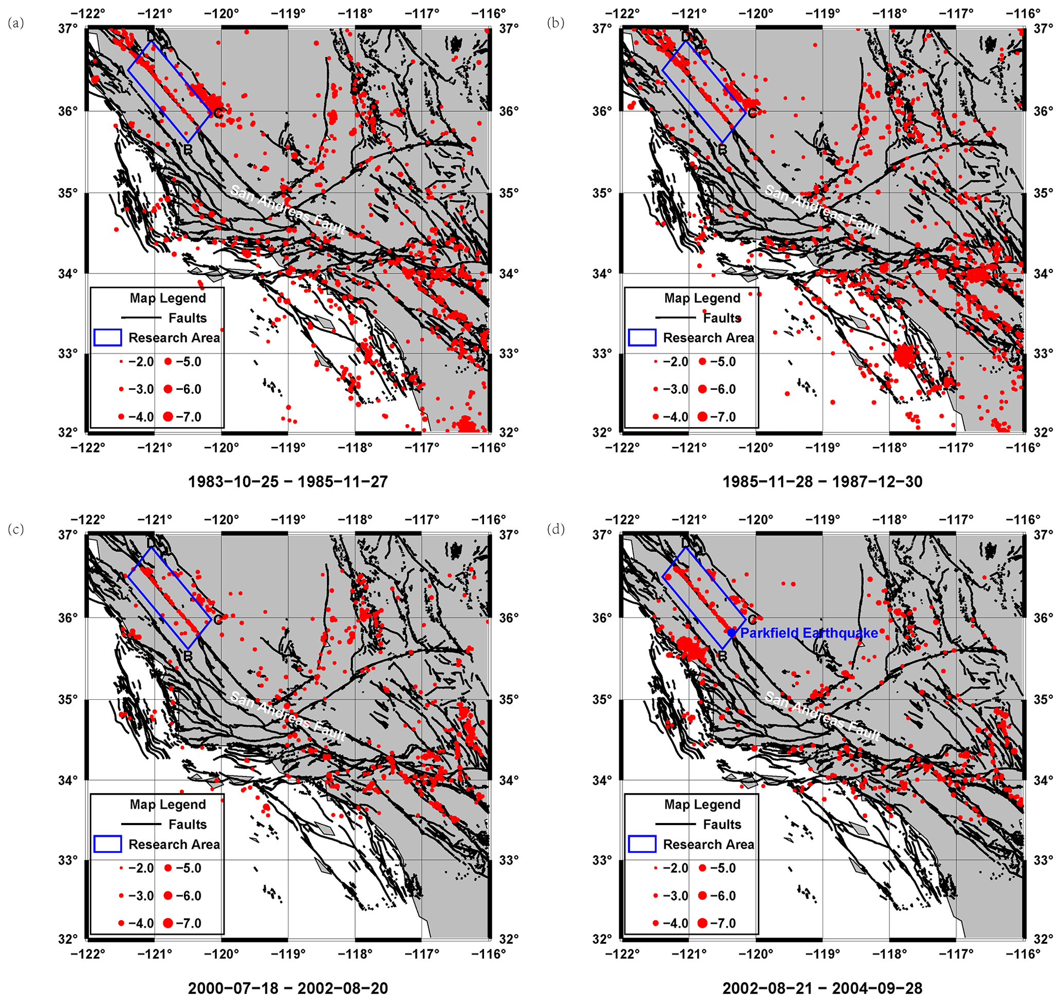
Figure 5The seismicity of the research area and surrounding area in a seismic cycle. The red points indicate the epicenters of earthquakes in the corresponding time. The location of the San Andreas Fault and the epicenter of the Parkfield earthquake are indicated on the map by white and blue fonts, respectively. The corresponding time is shown under each image. (a) Seismicity during 25 October 1983 to 27 November 1985. (b) Seismicity during 28 November 1985 to 30 December 1987. (c) Seismicity of the research area and surrounding area during 18 July 2000 to 20 August 2002. (d) Seismicity of the research area and surrounding area during 21 August 2002 to 28 September 2004.
At each stage, there are many earthquakes with magnitude less than 5 in the study area, and many of them distribute along the fault in the research area. Qualitatively, this is consistent with the experimental results. Quantitatively, if these small earthquakes are compared with the sampling points with large deformation, whether the average distance between these small earthquakes and the fault zone is consistent with the experimental results will be essential.
2.5 Seismic monitoring models
The CV results calculated by the differential maximum principal strain in the experiments show that the marble samples with prefabricated cracks have obvious precursor characteristics before rupture, so it is essential to arrange the seismic monitoring stations to capture such features. Three seismic monitoring models are proposed here, and their monitoring effects are judged. (1) Seismic stations are uniformly distributed in the study area. (2) Seismic stations are densely distributed along the fault zone, and the further away from the fault zone, the sparser the distribution of the stations along the direction parallel to the fault zone. The spacing of the stations along the direction perpendicular to the fault zone remains unchanged. (3) Seismic stations are densely distributed in the direction perpendicular to the fault zone, and the further away from the fault zone, the sparser the distribution of the stations in the direction perpendicular to the fault zone. The spacing of the stations in the direction parallel to the fault zone remains unchanged. The designs of the models are shown in Fig. 6 (sample 4 is taken as an example, and other samples are shown in Appendix C, Figs. C1–C4).
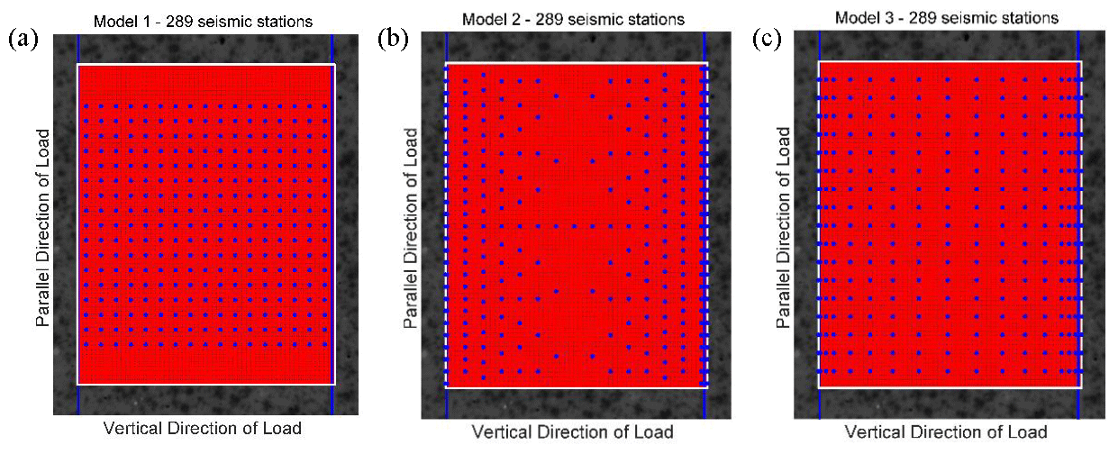
Figure 6Three kinds of seismic monitoring models with different numbers of seismic monitoring stations. Each figure shows the observational area of sample 4. The blue lines indicate the prefabricated cracks. The area enclosed by the white rectangle is the calculation area. The red points in the calculation area represent all the sampling points, while the blue points indicate the limited sampling points (seismic monitoring station) in different models. The horizontal axis is perpendicular to the direction of load, and the vertical axis is parallel to the direction of loading. (a) Model 1 with 289 seismic stations. (b) Model 2 with 289 seismic stations. (c) Model 3 with 289 seismic stations.
Using the differential maximum principal strain as the monitoring signal, simulate with these three models when the numbers of seismic stations are 289 (as shown in Fig. 6), 196, and 100 (as shown in Fig. S5 in the Supplement), respectively. By comparing the CV obtained from monitoring all sampling points and limited sampling points of different models, which model is more suitable for guiding the distribution of seismic stations and monitoring the precursory features of fracture and earthquakes is determined.
One of the starting points of this paper is to explore whether the marble rocks with prefabricated cracks have precursors before fracture. To investigate this, different kinds of CV are calculated with different physical quantities obtained by the DSCM, and the fluctuation of each CV with the increase in load is observed. Our results show that each CV is fluctuating with an obvious jump in the loading process. Thus, we have selected the differential maximum principal strain with the most obvious characteristics as an example to show this. Besides, the locations of sampling points with large differential maximum principal strain exceeding the threshold at different loading stages are shown in Fig. 4 and Appendix B. The positions of such points change with the increase in load and gradually move towards the precast cracks. We compare this feature with the seismicity in and around the northern end of the SAF in California in order to establish a connection between experimental observation and natural observation. Finally, the differential maximum principal strain is taken as the monitoring signal to explore how to use limited stations to monitor the precursor characteristics more effectively.
3.1 Precursor characteristics
There are many physical quantities obtained by the DSCM, including displacement and strain. We have used the proposed method in Sect. 2.3 to gain the corresponding differential values and compute the CV of these differential values, which are shown in Fig. 3. It can be seen obviously from Fig. 3 (and Appendix A) that each CV curve shows at least one jump during loading, which is the so-called precursor characteristics. Here, the CV calculated by the differential maximum principal strain is taken as an example to illustrate these precursor characteristics, because it has physical significance and obvious consequence.
The CVs of these five samples have a common background value (about 0.5) shown in Fig. 7, which proves the CV is a statistic that can be used to describe the characteristics of different samples. Besides, each CV curve fluctuates with the increase in load, and some of them reach the largest level at 60 %–80 % fracture load, while others reach 80 %–100 %. We believe that the reason for this difference is the uniqueness of each sample, which includes micro-cracks, porosity, joints, and so on. During direct shear, joints dilate before slip (Goodman, 1970; Goodman and Ohnishi, 1973), and even after many stick-slip cycles a small amount of dilation is observed before each event (Sundaran et al., 1976). Therefore, it is reasonable to believe that cracks begin to form in samples when the CV reaches a high level, and local deformation is relatively large and concentrated at this time. When the cracks are connected, the whole sample will rupture. Obviously, the CV indicates the development of cracks in the samples, and it is sensitive to deformation within the rocks.
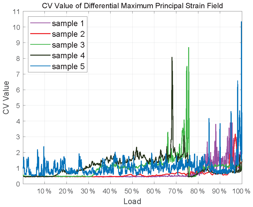
Figure 7The CV of differential maximum principal strain fields for the five samples. The colored lines represent the CV calculated by differential maximum principal strain fields of different samples.
3.2 Comparison with nature seismicity
By observing the CVs of different samples, we set different thresholds for these samples and mark the sampling points with large differential maximum principal strains that exceed the corresponding threshold on each sample's surface at different loading stages (Fig. 4 and Appendix B). It can be seen clearly from these results that the positions of these sampling points may be disordered at the beginning. This disorder is not truly disordered but is actually affected by the development of cracks and stress concentrations inside the rock during loading. When the rock is close to the rupture stage, these large deformation points appear around the precast cracks. Therefore, it is necessary to investigate the changes in the average distance between these points and the precast cracks as the load increases if we want to know whether the locations where these points appear are regular. We calculate the distance between these points and the right precast crack of each sample, since most of these points are concentrated on the right crack at the final stage. Furthermore, understanding the relationship between the locations of small earthquakes (magnitude < 5) and faults, before moderate and strong earthquakes (magnitude ≥ 5), is also the key to connecting the experimental results with the natural observations. Thus, the experimental results are compared with the seismicity of the northern end of the SAF and its surrounding area (the research area), and whether these two have similar characteristics is analyzed.
When there is no sampling point with large differential maximum principal strain satisfying the judge condition (we set for each sample in Sect. 2.4) in the corresponding loading stage, we assumed that the average distance from these sampling points to the right precast crack in this stage is zero. The results obtained under this assumption are shown in Fig. 8. It can be seen from Fig. 8 that the average distances of most samples and natural earthquakes are relatively stable at the 40 %–60 % loading stage, and then the distance changes dramatically as the load increases. For some samples (sample 3 and sample 5), there is a peak at the 90 % loading stage, which is consistent with the actual result in Fig. 8b. Finally, as the fracture approaches, the average distance between the sampling points with large differential maximum principal strain of all the samples and the right prefabricated crack become small, which proves that these sampling points are clustered around the crack at last. It is worth noting that the results of all samples are close to the same value at the 100 % loading stage, which also indicates that the sampling points meeting the judge condition are concentrated around the right prefabricated crack and that the concentration degree is nearly the same. The actual result in Fig. 8b shows that the positions of small earthquakes converge towards the fault with the approach of moderate and strong earthquakes, which is also the same as the experimental results. In particular, the result of sample 5 shows a striking similarity to the actual result. A very important phenomenon here is that the maximum values of these distances occur at a certain stage rather than the initial stage of loading. This means that a moderate or strong earthquake near the fault is possible soon after many small earthquakes have occurred in places far from the fault. This will be helpful to understand the development of ground strain and spatial evolution characteristics of earthquakes.

Figure 8Changes in distance. (a) The average distance between the positions of the sampling points with large differential maximum principal strain and the right precast crack. The colored lines represent the results of different samples. (b) The average distance between the small earthquakes (magnitude < 5) and the northern end of the SAF in the research area.
3.3 Comparison of seismic monitoring models
After showing the precursor characteristics of fracture, how to monitor this kind of precursory signal effectively becomes quite significant. Three commonly used seismic monitoring models are presented in Sect. 2.5. In fact, these three models are equivalent to taking a limited number of sampling points in the calculation area of the sample surface in three different ways. Here, the differential maximum principal strain of the chosen sampling points is used as the monitoring signal to compare the monitoring effects of these models. There are three steps to achieve this aim: firstly, calculate the CV of the limited sampling points monitored by the three models; secondly, calculate the CV of the full sampling points; finally, calculate the correlation coefficient of these two CVs with the following formula.
In this formula, is the mean differential maximum principal value of the limited sampling points (), and is the mean differential maximum principal value of the full sampling points (). The results are shown in Table 2.
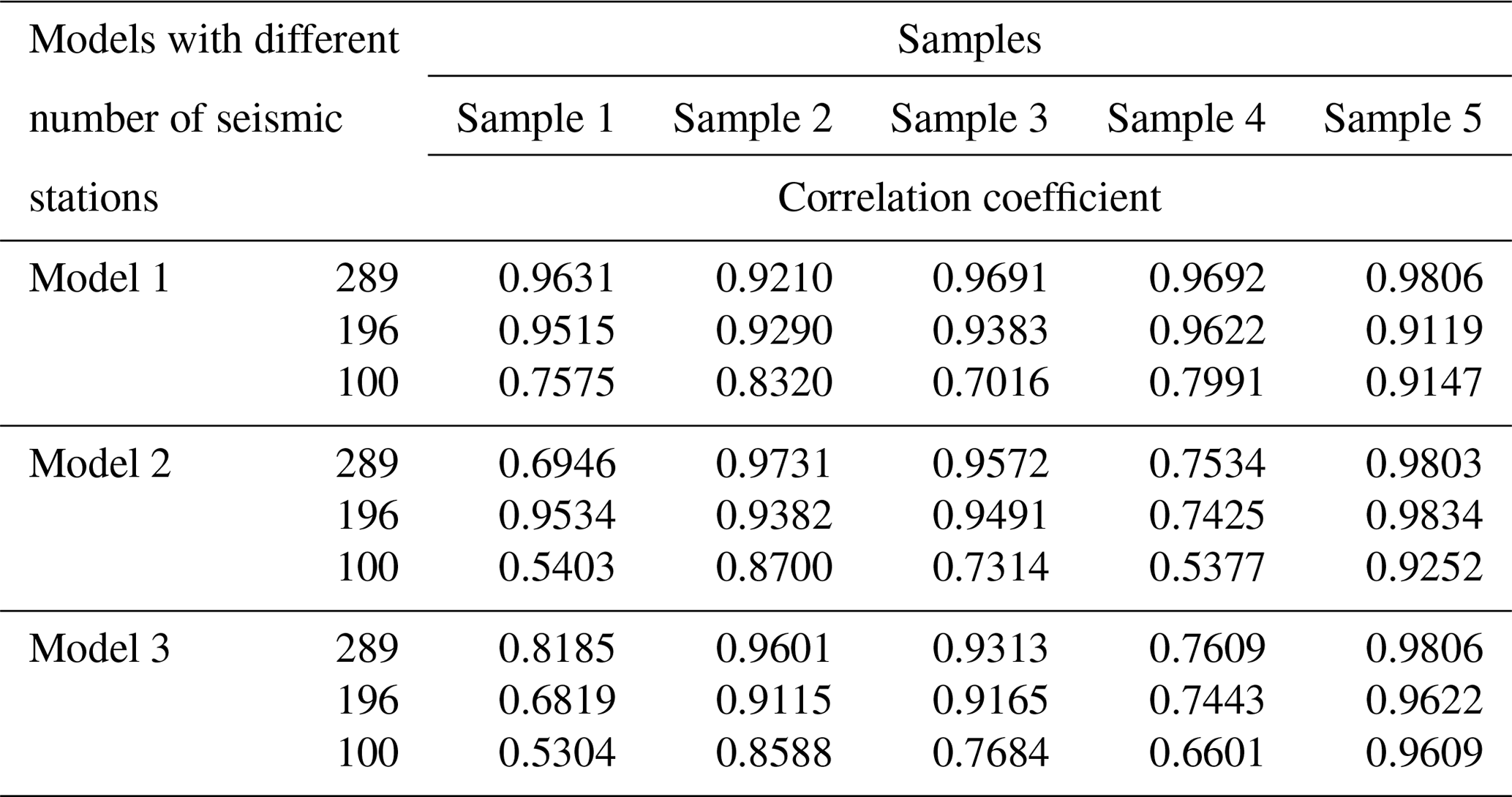
Generally, when the number of seismic stations is sufficient (≥289), arranging stations uniformly like Model 1 throughout the research area is the best way to monitor the precursory signal because most of the corresponding correlation coefficients give the highest values. When the number of seismic stations is relatively small (196 seismic stations), the monitoring effect of Model 2 is the best, even better than that of Model 1. When the number of seismic stations continues to decrease (less than 100), the monitoring effects of the three models have almost no difference. Therefore, these three models are suitable for different situations. In the case of a small number of seismic stations, selecting any model is fine due to the similar monitoring effect. As the number of stations increases, the advantages of Model 2 and Model 1 begin to emerge. According to this study, a more appropriate way to arrange seismic stations can be chosen in field work.
4.1 The CV fluctuates with the increase in load
It is apparent that the CVs of different samples do fluctuate with the increase in load and appear to dramatically jump. Simultaneously, some of these jumps occur at the 60 %–80 % loading phase, while the others happen at the 80 %–100 % loading stage. Although the existence of premonitory characteristics is proven by these jumps, the curve features of each CV are not the same. Each one has its own maximum value and fluctuation characteristics, which is why we set various thresholds to find large deformation sampling points on different sample surfaces. The causes of the distinctions are worth pondering. The main reasons for these dissimilarities are the inherent properties of the samples, including porosity, connectivity, and degree of joint development. As the crack density increases, the crack interactions become more significant (Sieradzki and Li, 1986), which is responsible for the rupture. Thus, the first obvious CV jumps occurring during diverse loading phases of the curves for these samples reveal the initial inherent level of crack density inside the samples when other properties are the same for all the samples. It is not only porosity that affects the characteristics of the CV curves, but also connectivity and degree of joint development. The higher they are, the smaller the maximum value of the CV will be and vice versa.
Another special phenomenon of CV curves is that each curve leaps significantly during a specific period of the whole loading stage. Some of them reach a high level at the 60 %–80 % loading stage, while the others jump at the 80 %–100 % loading stage. If we regard the sample fracture as a main earthquake, then this kind of jump is a concentrated release of stress, resulting in the emergence of large deformation sampling points that can be considered some small earthquakes before the main shock. The occurrence time of the CV jumps suggests that these small earthquakes can be triggered much earlier or just a little earlier than the main shock. When the former occurs, there will be a period of quiescence before the main earthquake, and if the latter happens, there will be an increase in seismicity before the main shock. The law of seismicity shows that before the occurrence of a large earthquake, the small earthquake activity may increase rapidly, decrease or even calm (Wyss, 1997) in the near-epicenter area of the large earthquake. There is controversy about these two. Some researchers find that there may be an acceleration period of seismic activity rather than the quiescence before some violent earthquakes (Bowman and King, 2001; Chen, 2003). However, with the development of seismic monitoring methods and the improvement of the earthquake catalogue, more and more phenomena of quiescence before large earthquakes have been found (Wu and Chiao, 2006; Katsumata, 2011; Pu, 2018). The relationship between accelerating seismicity and quiescence is also highly regarded, as they are two major phenomena ahead of a main shock (Di Giovambattista and Tyupkin, 2004; Mignan and Di Giovambattista, 2008). The results of CVs in this paper also show these two precursory characteristics, which indicates that this statistic is effective in describing and extracting premonitory features of rock fracture.
4.2 Connection between experimental results and natural seismicity
In fact, our experiments aim to simplify the complex mechanism of natural seismicity around a strike-slip fault and simulate the deformation process in one seismic cycle. However, the scale and model problems need to be considered during this procedure, in which the scale problem refers to the conversion between laboratory scale and natural scale and the model question refers to whether the laboratory model can be used in nature. Therefore, we set the rectangular area with only one strike-slip fault shown in Fig. 5 as a study area to limit the influence of other faults around, so that the simulations of the experiments are consistent with the natural state in a certain extent, which help us to weaken the above two problems.
There are many similarities between some experimental results and actual results, including an increase in distance at the 90 % loading stage and a decrease at the 100 % loading stage, as shown in Fig. 8. However, some samples do not show such a remarkable increase and decrease, and the reason for this difference can be divided into two parts. The first part is relevant to intrinsic properties of the samples as detailed in Sect. 4.1, which is also the main reason for the causes of this dissimilarity. The second part may be related to the practical dimensions of the samples and the prefabricated cracks on these samples, but this part may have just a little influence because the errors are very small and within the permit. A convincing argument for observation is that the final results of all samples are very close, which indicates that the sampling points with large deformation gather around the precast crack at this time. Besides, some small earthquakes may occur a little farther from the fault before the main earthquake, and this is the meaning of the sudden jump at the 90 % loading stage shown in Fig. 8. Investigating whether other areas with a relatively stable seismic cycle and a strike-slip fault also have these features is a useful way to understand the seismogenic mechanism and the seismicity included in this phenomenon.
4.3 Effects of earthquake monitoring models
After finding that the CV is effective at characterizing the precursor of rock fracture and the experimental results have some common features with the natural seismicity results, we design three monitoring models to explore how to capture it more effectively. Under the premise that each sampling point is regarded as a seismic station, these three models are actually equivalent to extracting corresponding sampling points in three ways for monitoring. The monitoring effect is judged by the correlation coefficient between the CV calculated by differential maximum principal strain of limited sampling points and all the sampling points of the models. We set a different number of stations for each model to compare the monitoring effect of them comprehensively. There is no doubt that distributing stations evenly like Model 1 is the best way to seize these precursors, while the number of stations is sufficient. However, if the number of stations dwindles, unexpected results emerge. The monitoring effect of Model 1 no longer occupies a dominant position, and the effect of the distribution mode of Model 2 has surpassed that of Model 1. If the number of stations continues to decrease, the monitoring effect of the three models showed a little difference. Starting from the formula of the correlation coefficient, the high value can be achieved if the CV of the three models coincides with that of the full sampling points. Thus, the monitoring model can have a relatively high correlation coefficient as long as it can ensure that the ratio of the sampling points with large deformation and the sampling points with small deformation conforms to that of the full sampling points. In this case, arranging the limited seismic stations uniformly in the entire area is the best way to capture the precursors if the numbers of seismic stations are large enough. However, the number of stations is very small at present, so it is beneficial for field work to explore how to distribute stations. This is a simulation of the earthquake monitoring model with a limited number of stations, hoping to provide a little help for related work.
Experiment is an effective tool to understand the complex mechanism of natural earthquakes. We perform uniaxial loading on five marble samples with prefabricated cracks and obtain their differential displacement and strain fields at different loading stages. The CV obtained from the calculation of these fields confirms the existence of precursor characteristics before rock fracture. Using results of the CV to set different thresholds, we find that large deformed sampling points on each sample surface will migrate to prefabricated cracks when the sample is close to failure. Similar features have been found on the seismicity of the San Andreas Fault in the research area. This is an attempt to link the experiment with nature. All these results prove the validity of the CV and the credibility of the CV describing the precursors. Thus, in order to monitor the precursory characteristics of this kind of rupture more effectively, we have designed three commonly useable seismic monitoring models and compare the monitoring effects of these models under the condition of limited seismic stations. It is found that the results of Models 1 and 2 are generally better than Model 3. In the field work, the most proper arrangement of seismic stations shall be selected according to the conditions, including the number of stations and the geological situation.
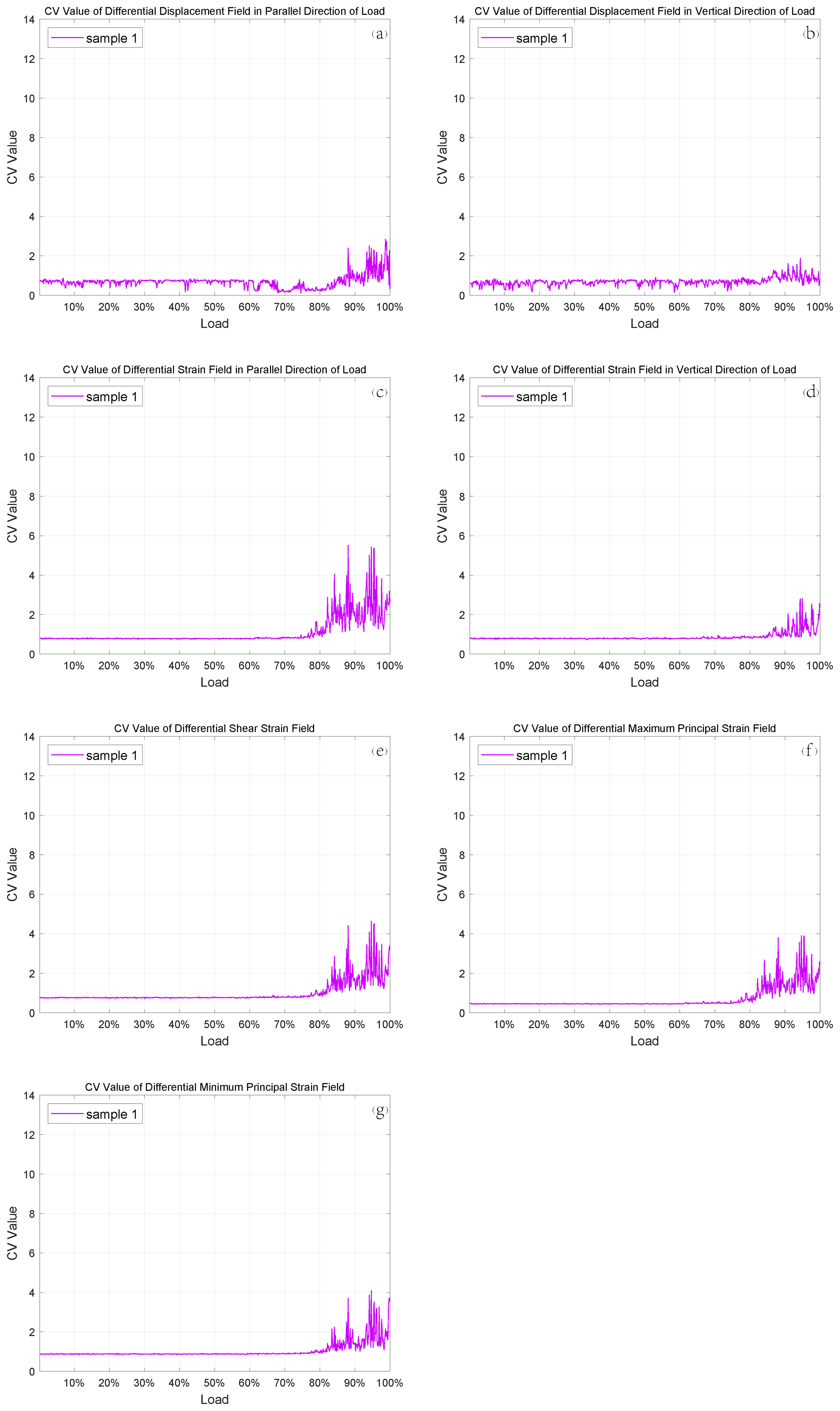
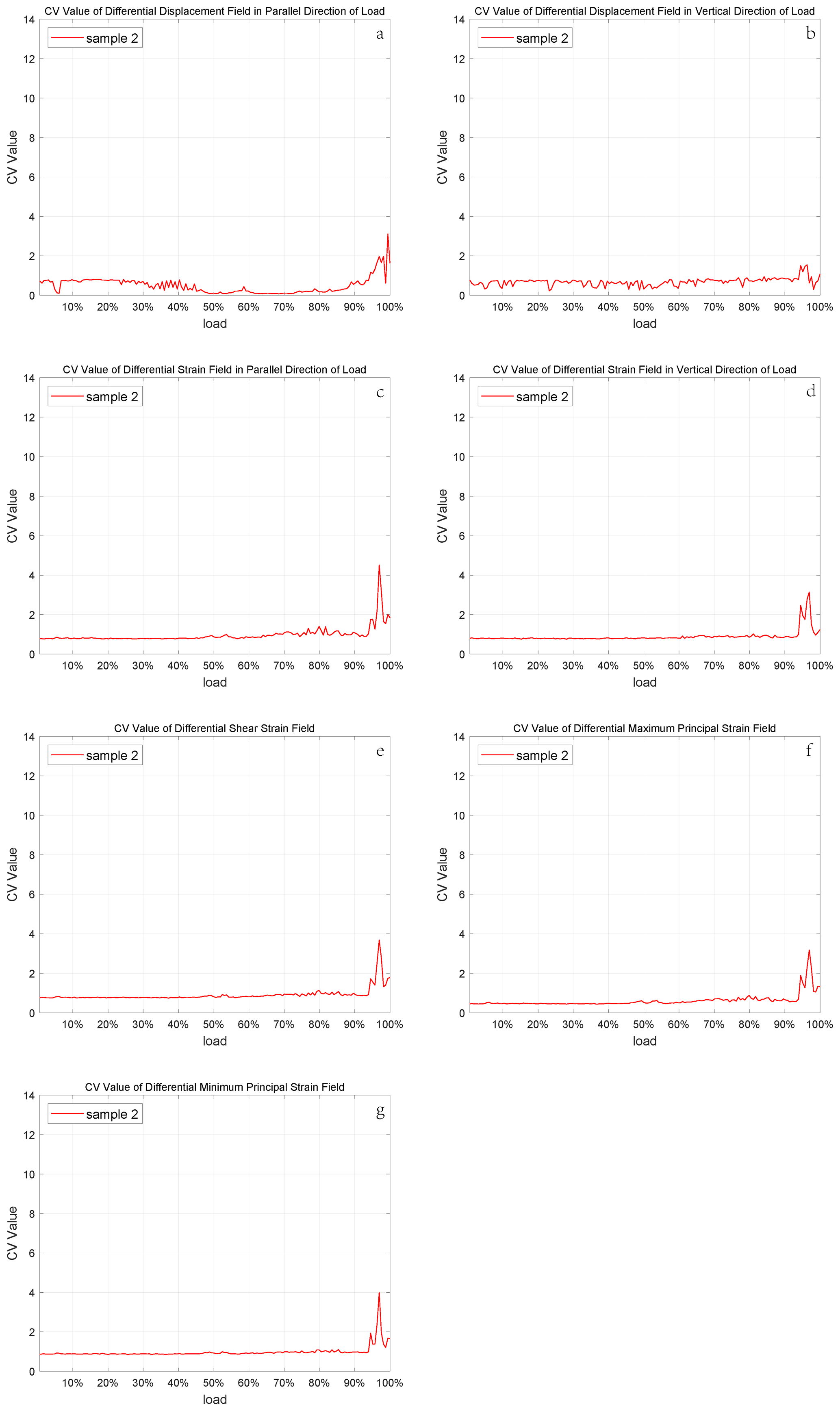
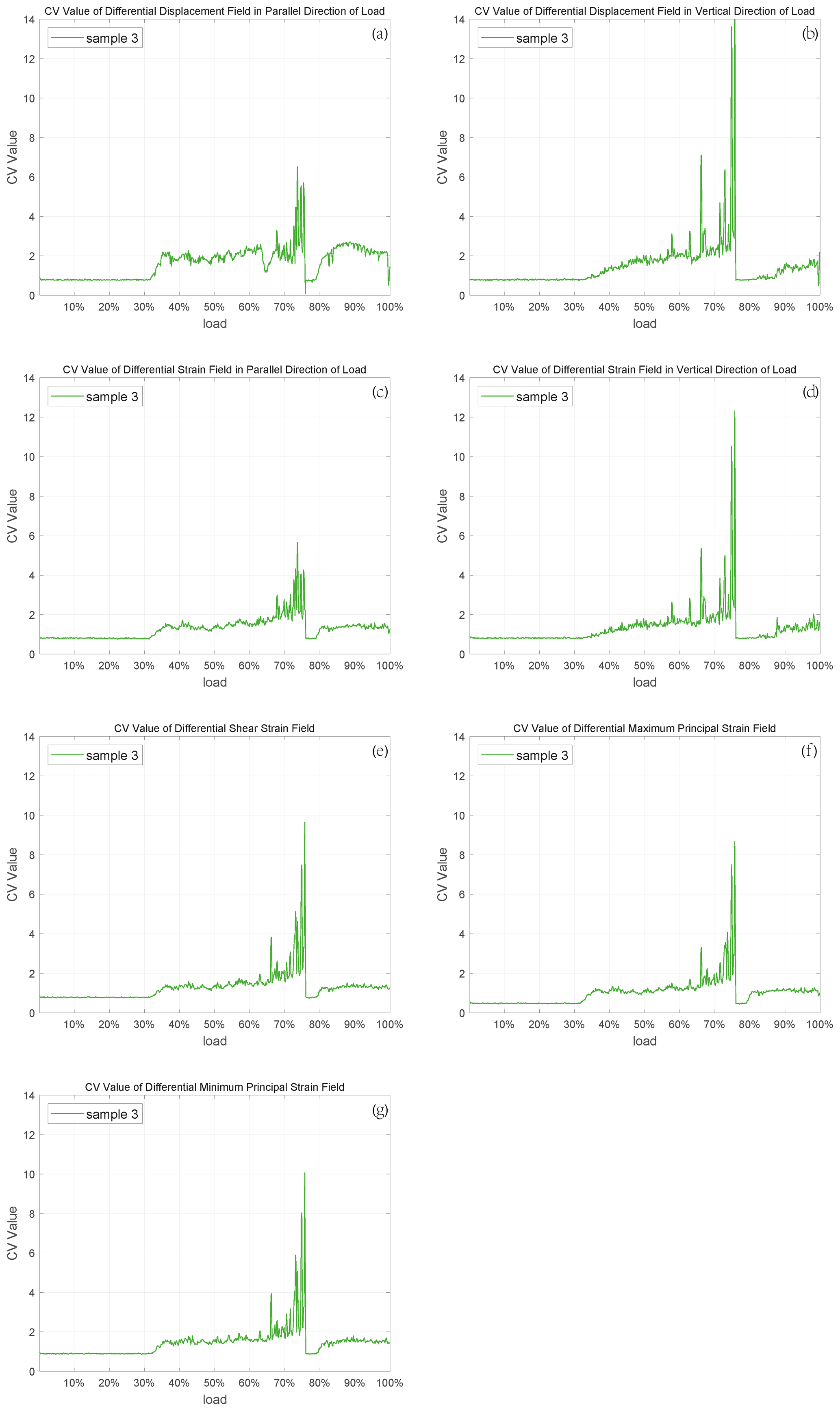
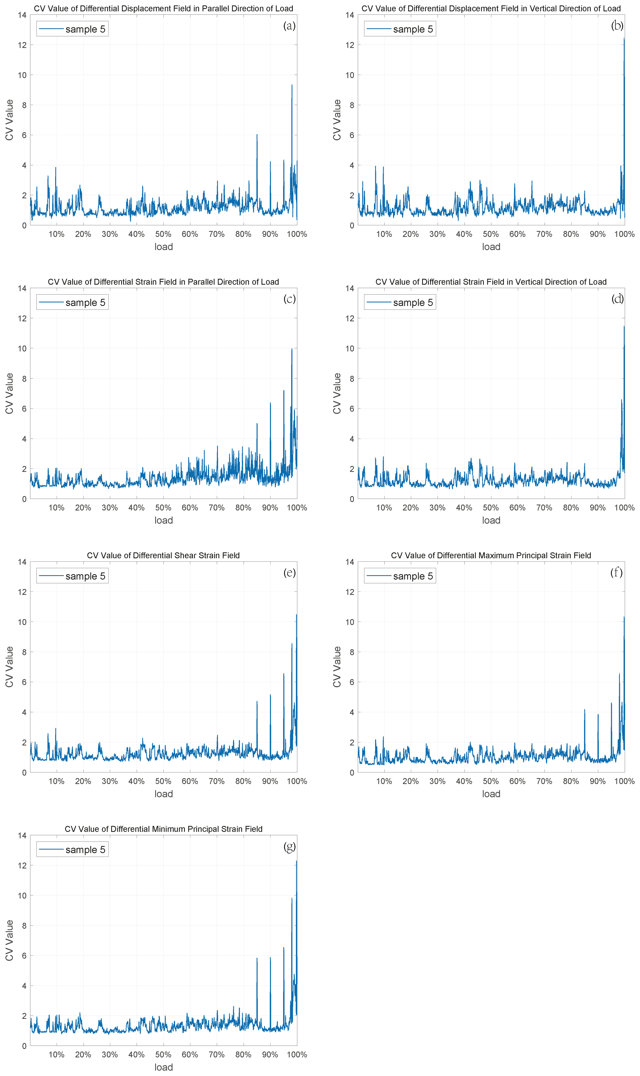

Figure B1The position of the sampling points with large differential maximum principal strain for sample 1. The blue lines indicate the prefabricated cracks. Each figure shows the observational area of sample 4 in the experiments. The area enclosed by the white rectangle is the calculation domain, and its size is constant in different loading stages. The red points represent the sampling points with large differential maximum principal strain that satisfy the judgment condition as the load increases (from a to j).
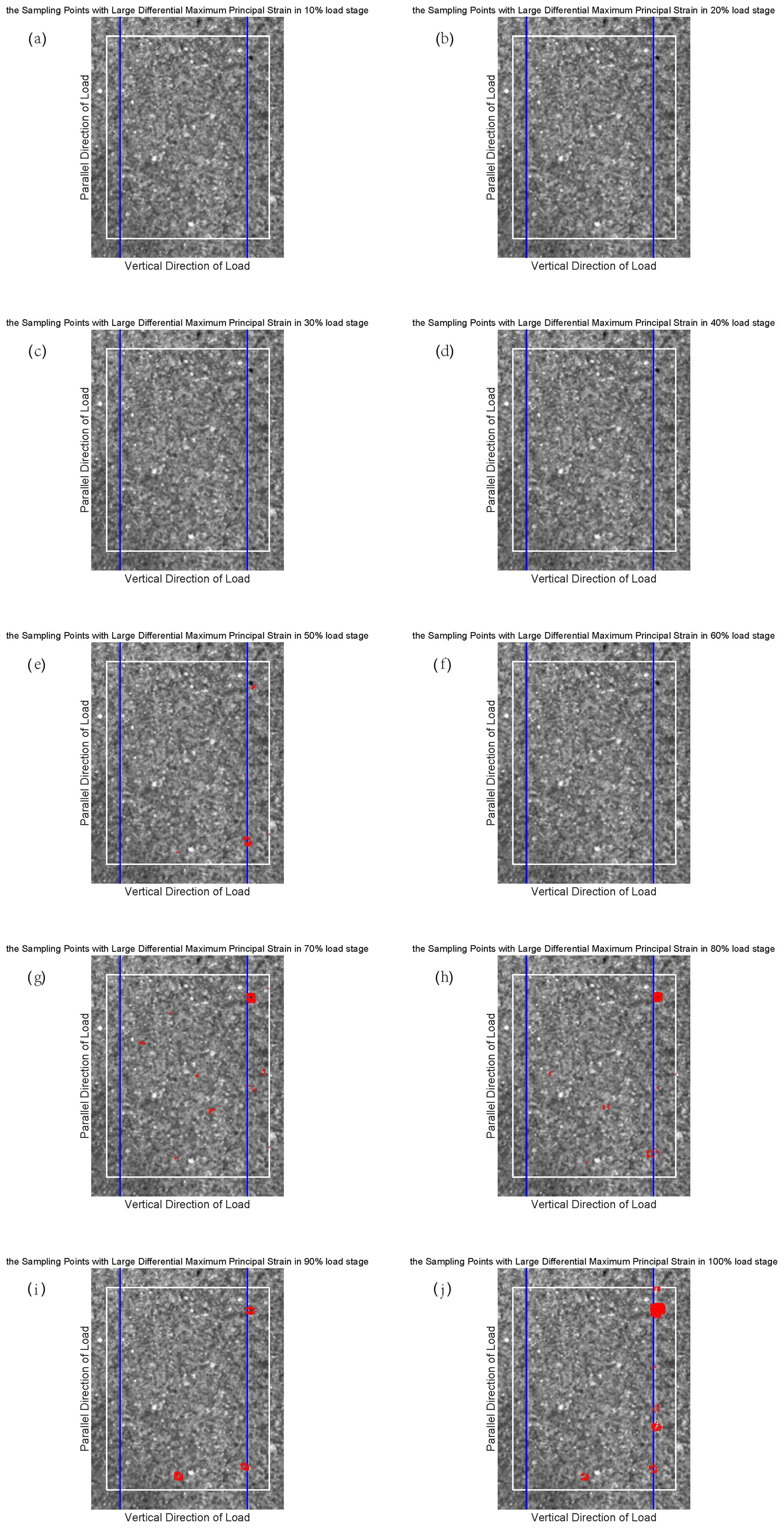
Figure B2The position of the sampling points with large differential maximum principal strain for sample 2.

Figure B3The position of the sampling points with large differential maximum principal strain for sample 3.
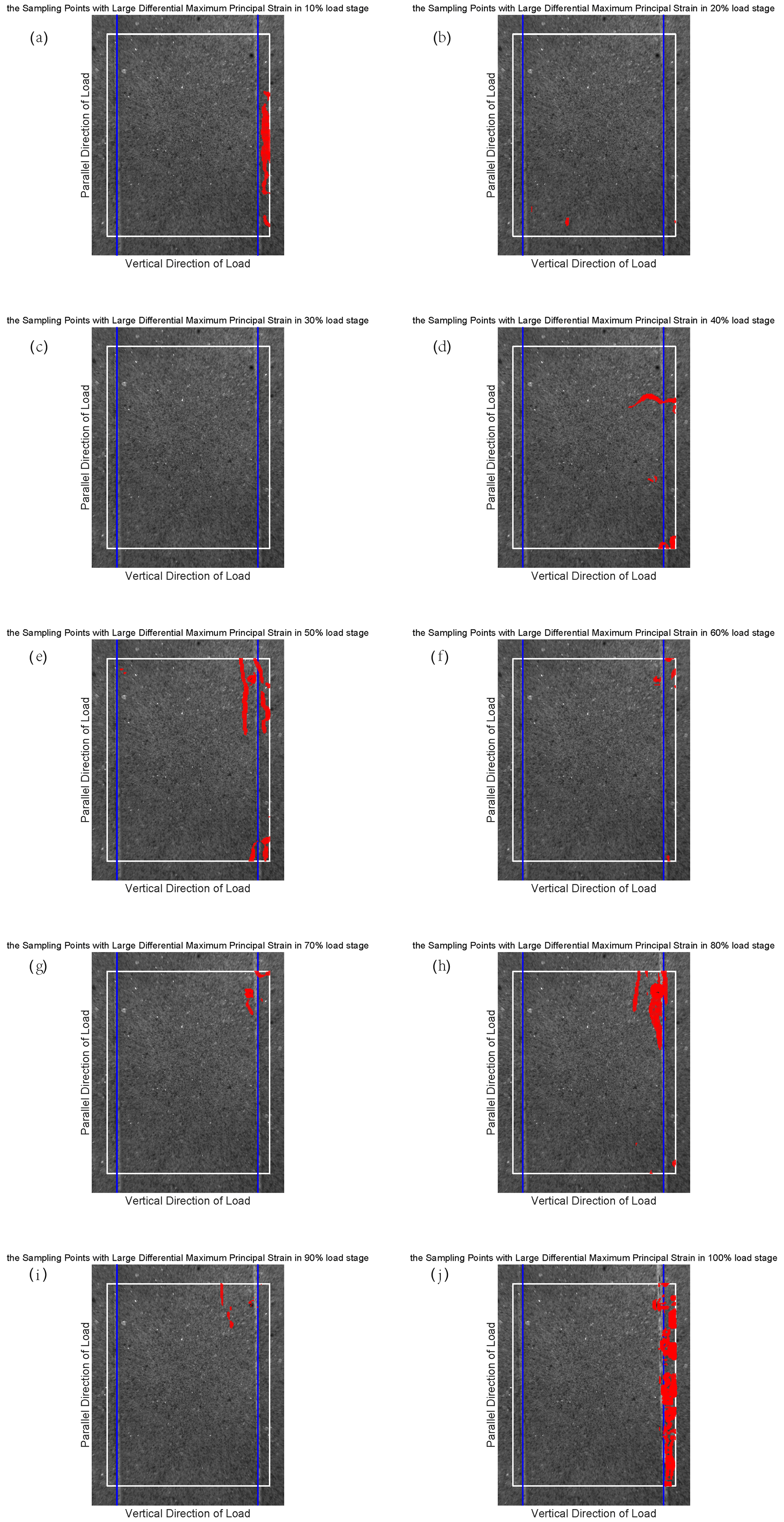
Figure B4The position of the sampling points with large differential maximum principal strain for sample 5.
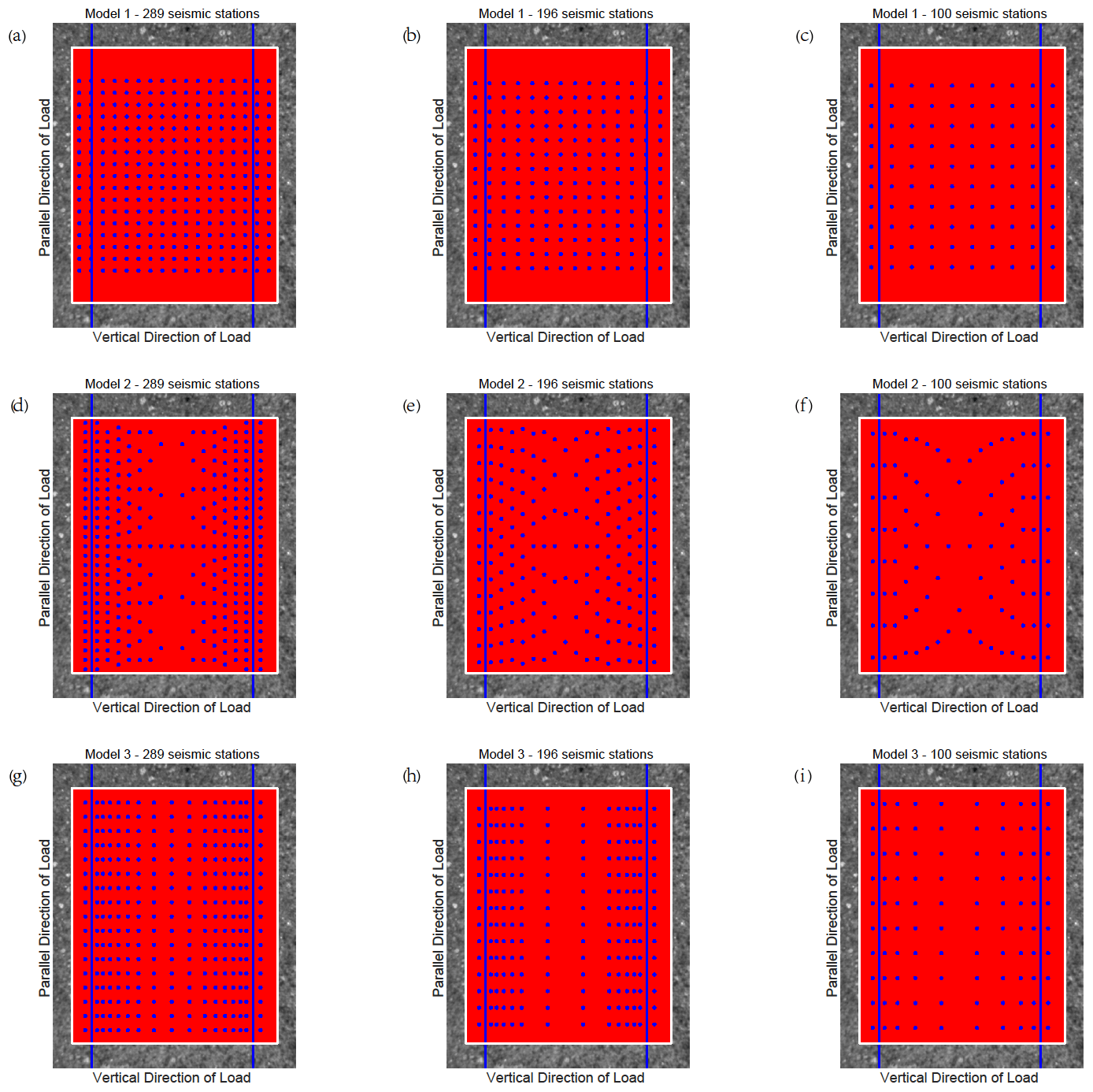
Figure C1Three kinds of seismic monitoring models with different numbers of seismic monitoring stations for sample 1. The blue lines indicate the prefabricated cracks. Each figure shows the observational area of sample 1. The area enclosed by the white rectangle is the calculation area. The red points in the calculation area represent the sampling points. The blue points indicate the locations of seismic stations in different models. The horizontal axis is perpendicular to the direction of load. The vertical axis is parallel to the direction of loading. Subfigures represent various models with different numbers of seismic monitoring stations.
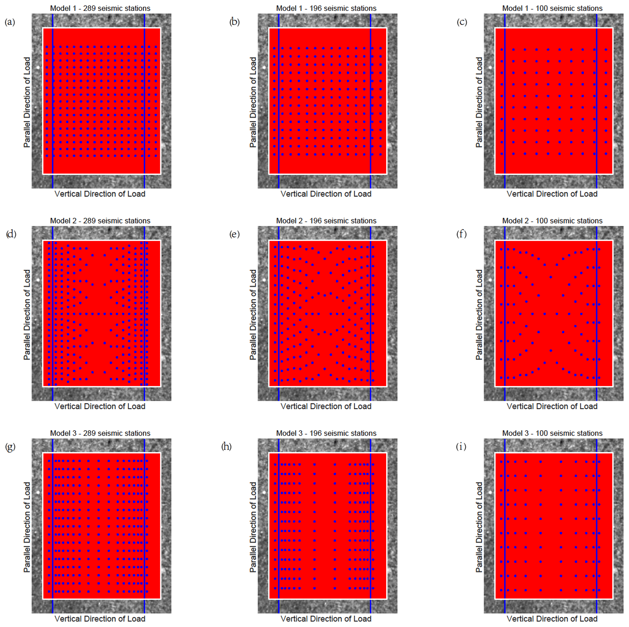
Figure C2Three kinds of seismic monitoring models with different numbers of seismic monitoring stations for sample 2.
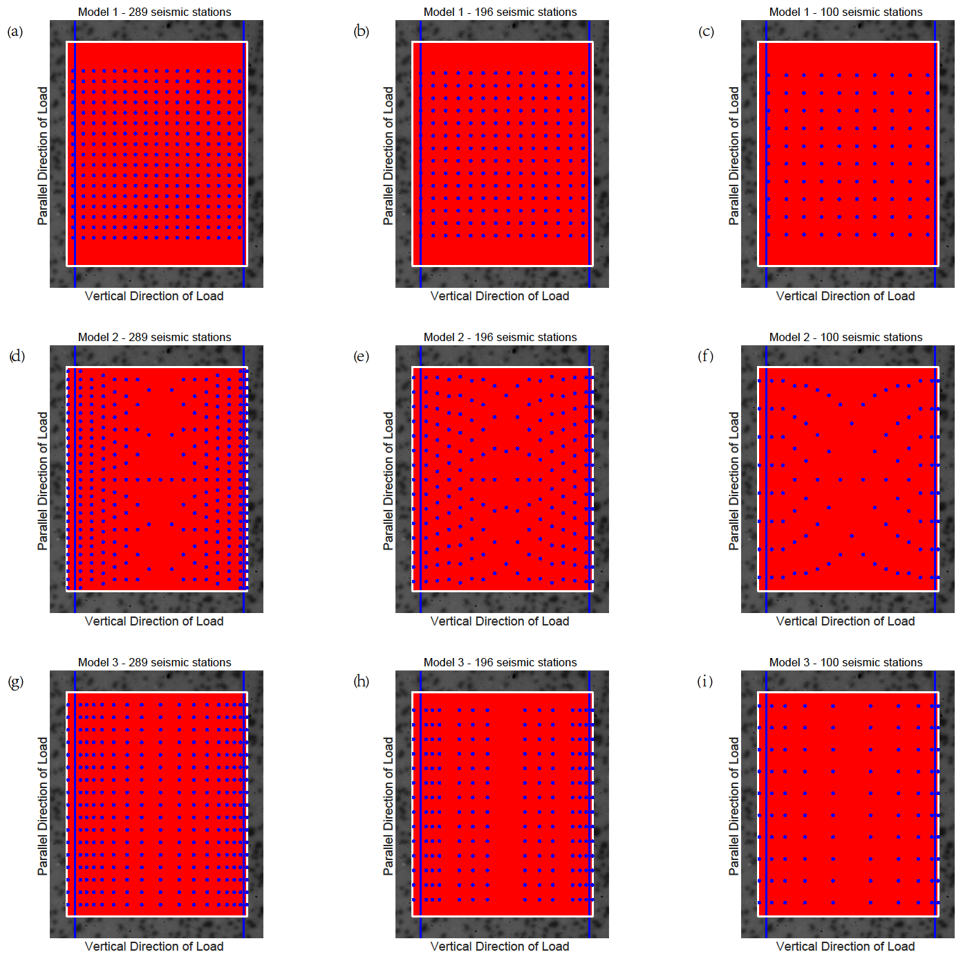
Figure C3Three kinds of seismic monitoring models with different numbers of seismic monitoring stations for sample 3.
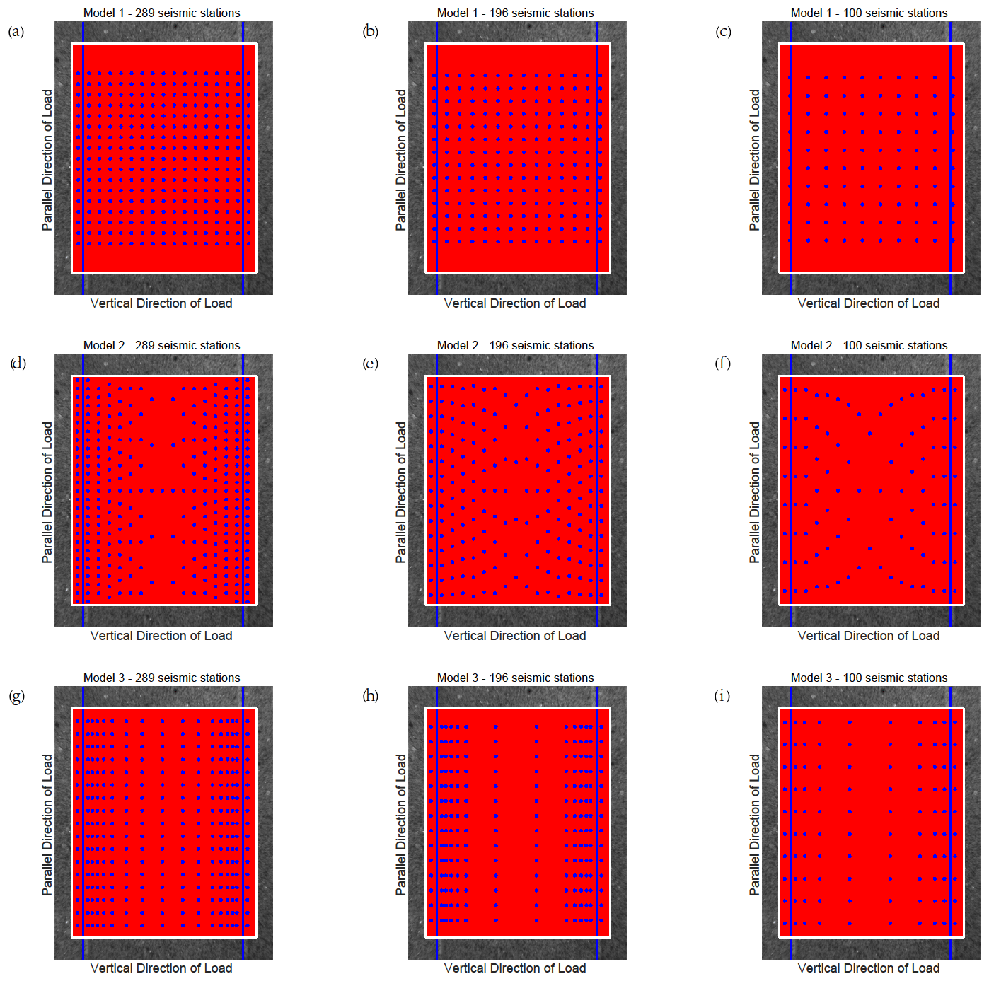
Figure C4Three kinds of seismic monitoring models with different numbers of seismic monitoring stations for sample 5.
Data are available upon request by contacting the corresponding author.
The supplement related to this article is available online at: https://doi.org/10.5194/npg-28-379-2021-supplement.
AX and YZ contributed to the conception of the study. AX performed all the experiments with JY, QZ and RL. AX also performed the data analysis and wrote the manuscript. MIE helped revise the manuscript.
The authors declare that they have no conflict of interest.
Publisher's note: Copernicus Publications remains neutral with regard to jurisdictional claims in published maps and institutional affiliations.
We thank all the people who were helpful to this article. This work was funded by the National Key Research and Development Program of China (grant nos. 2018YFC1504203 and SQ2017YFSF040025).
This research has been supported by the National Key Research and Development Program of China (grant nos. 2018YFC1504203 and SQ2017YFSF040025).
This paper was edited by Ilya Zaliapin and reviewed by two anonymous referees.
Aldamegh, K. S., Abou Elenean, K. M., Hussein, H. M., and Rodgers, A. J.: Source mechanisms of the June 2004 Tabuk earthquake sequence, Eastern Red Sea margin, Kingdom of Saudi Arabia, J. Seismol., 13, 561–576, https://doi.org/10.1007/s10950-008-9148-5, 2009.
Barbot, S., Lapusta, N., and Avouac, J. P.: Under the Hood of the Earthquake Machine: Toward Predictive Modeling of the Seismic Cycle, Science, 336, 707–710, https://doi.org/10.1126/science.1218796, 2012.
Beeler, N. M., Tullis, T. E., Kronenberg, A. K., and Reinen, L. A.: The instantaneous rate dependence in low temperature laboratory rock friction and rock deformation experiments, J. Geophys. Res.-Sol. Ea., 112, B07310, https://doi.org/10.1029/2005jb003772, 2007.
Bowman, D. D. and King, G. C. P.: Accelerating seismicity and stress accumulation before large earthquakes, Geophys. Res. Lett., 28, 4039–4042, https://doi.org/10.1029/2001gl013022, 2001.
Brace, W. F., Paulding, B. W., and Scholz, C.: Dilatancy in Fracture of Crystalline Rocks, J. Geophys. Res., 71, 3939–3954, https://doi.org/10.1029/jz071i016p03939, 1966.
Brady, B. T.: Laboratory investigations of tilt and seismicity anomalies in rock before failure, Nature, 260, 108–111, 1975.
Butler, R.: Composite earthquake source mechanism for 2018 Mw 5.2–5.4 swarm at Kīlauea Caldera: antipodal source constraint, Seismol. Res. Lett., 90, 633–641, https://doi.org/10.1785/0220180288, 2019.
Chen, C. C.: Accelerating seismicity of moderate-size earthquakes before the 1999 Chi-Chi, Taiwan, earthquake: Testing time-prediction of the self-organizing spinodal model of earthquakes, Geophys. J. Int., 155, F1–F5, https://doi.org/10.1046/j.1365-246x.2003.02071.x, 2003.
Davidsen, J., Stanchits, S., and Dresen, G.: Scaling and universality in rock fracture, Phys. Rev. Lett., 98, 125502, https://doi.org/10.1103/physrevlett.98.125502, 2007.
Davidsen, J., Kwiatek, G., Charalampidou, E. M., Goebel, T., Stanchits, S., Ruck, M., and Dresen, G.: Triggering Processes in Rock Fracture, Phys. Rev. Lett., 119, 068501, https://doi.org/10.1103/physrevlett.119.068501, 2017.
Dieterich, J. H.: Modeling of rock friction, 1: experimental results and constitutive equations, J. Geophys. Res., 84, 2161–2168, https://doi.org/10.1029/jb084ib05p02161, 1979.
Di Giovambattista, R. and Tyupkin, Y. S.: Seismicity patterns before the M=5.8 2002, Palermo (Italy) earthquake: seismic quiescence and accelerating seismicity, Tectonophysics, 384, 243–255, https://doi.org/10.1016/s0040-1951(04)00129-5, 2004.
Frohlich, C.: Display and quantitative assessment of distributions of earthquake focal mechanisms, Geophys. J. Int., 144, 300–308, https://doi.org/10.1046/j.1365-246x.2001.00341.x, 2001.
Frohlich, C. and Apperson, K. D.: Earthquake focal mechanisms, moment tensors, and the consistency of seismic activity near plate boundaries, Tectonics, 11, 279–296, https://doi.org/10.1029/91tc02888, 1992.
Goff, J. A., Bergman, E. A., and Solomon, S. C.: Earthquake source mechanisms and transform fault tectonics in the Gulf of California, J. Geophys. Res.-Solid, 92, 10485–10510, https://doi.org/10.1029/jb092ib10p10485, 1987.
Goodman, R. E.: The deformability of joints, ASTM, STP 477, Amer. Soc. For Testing Matls., 174–196, 1970.
Goodman, R. E. and Ohnishi, Y.: Undrained shear testing of jointed rock, Rock Mech., 5, 129–149, https://doi.org/10.1007/bf01238044, 1973.
Gutenberg, B. and Richter, C. F.: Frequency of Earthquakes in California, Nature, 156, 371, https://doi.org/10.1038/156371a0, 1945.
Harlin, G. and Willis, J. R.: The influence of crack size on the fracture behaviour of short cracks, Int. J. Fracture, 42, 341–355, https://doi.org/10.1007/978-94-017-2444-9_22, 1990.
Kagan, Y. Y.: 3-D rotation of double-couple earthquake sources, Geophys. J. Int., 106, 709–716, https://doi.org/10.1111/j.1365-246x.1991.tb06343.x, 1991.
Kagan, Y. Y.: Double-couple earthquake focal mechanism: random rotation and display, Geophys. J. Int., 163, 1065–1072, https://doi.org/10.1111/j.1365-246x.2005.02781.x, 2005.
Kagan, Y. Y.: Double-couple earthquake source: symmetry and rotation, Geophys. J. Int., 194, 1167–1179, https://doi.org/10.1093/gji/ggt156, 2013.
Kagan, Y. Y. and Jackson, D. D.: Long-Term Earthquake Clustering, Geophys. J. Int., 104, 117–133, 1991.
Kahir, A. W.: A study of acoustic emission during laboratory fatigue tests on Tennessee sandstone, in: Proc. First Conf. On Acoustic emission and microscopic activity in geologic structure and materials, The Pennsylvania State Univ, Trans. Tech. Publications, Clausthal, 58–86, 1977.
Kammer, D. S. and McLaskey G. C.: Fracture energy estimates from large-scale laboratory earthquakes, Earth Planet. Sc. Lett., 511, 36–43, https://doi.org/10.1016/j.epsl.2019.01.031, 2019.
Kammer, D. S., Svetlizky, I., Cohen, G., and Fineberg, J.: The equation of motion for supershear frictional rupture fronts, Sci. Adv., 4, 12784–12792, https://doi.org/10.1126/sciadv.aat5622, 2018.
Katsumata, K.: Precursory seismic quiescence before the Mw=8.3 Tokachi-oki, Japan, earthquake on 26 September 2003 revealed by a re-examined earthquake catalog, J. Geophys. Res.-Sol. Ea., 116, B10307, https://doi.org/10.1029/2010jb007964, 2011.
Lockner, D. and Byerlee, J.: Acoustic emission and creep in rock at high confining pressure and differential stress, B. Seismol. Soc. Am., 67, 247–258, https://doi.org/10.1016/0148-9062(78)91004-5, 1977.
Lockner, D. A., Byerlee, J. D., Kuksenko, V., Ponomarev, A., and Sidorin, A.: Quasi-Static Fault Growth and Shear Fracture Energy in Granite, Nature, 350, 39–42, https://doi.org/10.1038/350039a0, 1991.
Ma, S. P., Xu, X. H., and Zhao, Y. H.: The Geo-DSCM system and its application to the deformation measurement of rock materials, Int. J. Rock Mech. Min., 41, 411–412, https://doi.org/10.1016/j.ijrmms.2004.03.056, 2004.
Mignan, A. and Di Giovambattista, R.: Relationship between accelerating seismicity and quiescence, two precursors to large earthquakes, Geophys. Res. Lett, 35, 563–575, https://doi.org/10.1029/2008gl035024, 2008.
Nur, A.: Dilatancy, Pore Fluids, and Premonitory Variations of Ts-Tp Travel Times, B. Seismol. Soc. Am., 62, 1217–1222, 1972.
Obert, L.: The microseismic method: discovery and early history, in: Proc. First Conf. on Acoustic emission microseismic activity in geologic structures and materials, , The Pennsylvania State Univ., Trans. Tech. Publications, 72, 11–12, 1977.
Paterson, M. S. and Olgaard, D. L.: Rock deformation tests to large shear strains in torsion, J. Struct. Geol., 22, 1341–1358, https://doi.org/10.1016/s0191-8141(00)00042-0, 2000.
Peters, W. H. and Ranson, W. F.: Digital image techniques in experimental stress analysis, Opt. Eng., 21, 427–431, 1982.
Pu, H. C.: Spatial and Temporal Characteristics of the Microseismicity Preceding the 2016 ML 6.6 Meinong Earthquake in Southern Taiwan, Pure Appl. Geophys., 175, 2077–2091, https://doi.org/10.1007/s00024-018-1801-5, 2018.
Rubin, A. M.: Episodic slow slip events and rate-and-state friction, J. Geophys. Res.-Sol. Ea., 113, B11414, https://doi.org/10.1029/2008jb005642, 2008.
Ruina, A. L.: Slip instability and state variable friction laws, J. Geophys. Res., 88, 10359, https://doi.org/10.1029/jb088ib12p10359, 1983.
Scholz, C. H.: Experiment study of the fracturing process in brittle rock, J. Geophys. Res., 73, 1447–1454, 1968.
Sieradzki, K. and Li, R.: Fracture-Behavior of a Solid with Random Porosity, Phys. Rev. Lett., 56, 2509–2512, https://doi.org/10.1103/physrevlett.56.2509, 1986.
Sundaran, P. N., Goodman, R. E., and Chiyuen, W.: Precursory and coseismic water pressure variations in stick-slip experiment, Geology, 4, 108–110, 1976.
Thurber, C., Roecker, S., Zhang, H., Baher, S., and Ellsworth, W.: Fine-scale structure of the San Andreas fault zone and location of the SAFOD target earthquakes, Geophys. Res. Lett., 31, L12S02, https://doi.org/10.1029/2003gl019398, 2004.
Wu, Y. M. and Chiao, L. Y.: Seismic quiescence before the 1999 Chi-Chi, Taiwan, Mw 7.6 earthquake, B. Seismol. Soc. Am., 96, 321–327, https://doi.org/10.1785/0120050069, 2006.
Wyss, M.: Case 23: Nomination of precursory seismic quiescence as a significant precursor, Pure Appl. Geophys., 149, 79–113, 1997.
Xia, K., Rosakis, A. J., and Kanamori, H.: Laboratory earthquakes: the sub-Rayleigh-to-supershear rupture transition, Science, 303, 1859–1861, http://www.jstor.org/stable/3836516 (last access: 29 July 2021), 2004.
Xia, K. W., Rosakis, A. J., Kanamori, H., and Rice, J. R.: Laboratory earthquakes along inhomogeneous faults: Directionality and supershear, Science, 308, 681–684, http://www.jstor.org/stable/3841995 (last access: 29 July 2021), 2005.
Yamaguchi, I.: A laser speckle strain gage, J. Phys. E Sci. Instrum., 14, 1270–1273, 1981.
- Abstract
- Introduction
- Methods
- Results
- Discussion
- Conclusions
- Appendix A: CV images of the other samples
- Appendix B: The position of the sampling points with large differential maximum principal strain for the other samples changes with load
- Appendix C: Three kinds of seismic monitoring models with different numbers of seismic monitoring stations for all of the samples
- Data availability
- Author contributions
- Competing interests
- Disclaimer
- Acknowledgements
- Financial support
- Review statement
- References
- Supplement