The impact of entrained air on ocean waves

We make a physical–mathematical analysis of the implications that the presence of a large number of tiny bubbles may have, when present, on the thin upper layer of the sea. In our oceanographic example, the bubbles are due to intense rain. It was found that the bubbles increase momentum dissipation in the near surface and affect the surface tension force. For short waves, the implications of increased vorticity are momentum exchanges between wave and mean flow and modifications to the wave dispersion relation. For the direct effect we have analyzed, the implications are estimated to be non-significant when compared to other processes of the ocean. However, we hint at the possibility that our analysis may be useful in other areas of research or practical application.

1 Introduction

Our interest is in the consequences of intense rain on the small-scale roughness of the ocean surface. More specifically, we analyze how the presence of tiny, rain-induced air bubbles in the thin upper layer of the ocean affects the high-frequency tail of the gravity wave spectrum, including capillary waves. Although tiny, both in length and height, with respect to the majestic motion of the surface, these waves are important for both physical and practical reasons. Physically, they control a large part of the exchanges between ocean and atmosphere, and they act as roughness elements for atmospheric turbulence and modulate the interaction between longer waves, currents, and wind (e.g., Ayet et al., 2020). At the same time, their presence is what allows the scatterometers to measure, globally, the winds on the ocean (Kudryavtsev et al., 1999).

The disappearance of capillary sea waves with rain is not new. Known to mariners since their early attempts (reduced small-scale roughness leads also to reduced breaking), the subject has also been studied in recent times by, e.g., Le Méhauté and Khangaonkar (1990) and Cavaleri et al. (2018). The former authors focused on the mechanical action of rain on the dynamics of the wave orbital motion. The latter authors' attention, taking the wavelets attenuation as a de facto evidence, focused more on the implications for air–sea interactions. In this work, we try to clarify one of the reasons why rain attenuates surface wavelets. Granted, if strong enough, the raindrops' mechanical action and induced turbulence, we focus our attention on the rain-induced presence of a large number of tiny air bubbles just below the surface (a few centimeters) and on how they affect the wave motion. To avoid the dominance of other processes, we exclude stormy conditions, considering either only swell or calm sea cases, but with enough wind to lead to waves on the surface. As for rain, just to frame the order of magnitude, under an intense rain with, e.g., 100 mm h⁻¹, assuming 4 mm diameter raindrops (volume $\mathrm{3}\times {\mathrm{10}}^{-\mathrm{6}}$ m³), this translates into 100 drops per square meter per second. Wolf (2001) suggests that, under these conditions, air injected into the sea can be a few cubic centimeters per square meter per second. Compared to other mechanisms that introduce air into the sea, one can conclude that rain contribution is very small. In general, this is true of quantitative terms, and we consider the process interesting from the physical point of view and with potential application in other practical fields.

On this basis, we make a physical–mathematical analysis of the ensuing processes. In Sect. 2, we propose a model that suggests how the entrainment of air leads to an increase in the effective viscosity of the upper ocean. We then use results from ocean acoustics (see Oguz and Prosperetti, 1990 and Prosperetti and Oguz, 1993) to compute the distribution of air bubbles for a given rain rate (Sect. 3). How changes of effective viscosity affect gravity waves is taken up in Sect. 4. It is found that, under vigorous rains, the air concentration due to air bubbles near the surface is capable of producing a damping effect akin to the (idealized) contamination of a free surface. A discussion of the results and conclusions and possible extensions of the present work appear in Sects. 5 and 6.

2 The dynamical approach and the presence of bubbles

To determine the impact of air bubbles on the thin upper level of the ocean, we perform homogenization on the Navier–Stokes equations. Homogenization is a well-established technique in modeling transport in complex media, endowed with statistical homogeneity in the media, as viewed at large scales (see Babuška, 1976; Bensousan et al., 1978; Cioranescu and Donato, 1999).

We assume that air bubbles are distributed uniformly in the transverse direction within the vicinity of the ocean surface. For our specific example, we explore how the presence of bubbles affects the effective viscosity of the fluid averaged over a cell Ω, of size ℓ³ (sub-wave scale), over which the distributions of the density and viscosity of the combined water and air bubble mixture are statistically stationary. The typical sub-wave speed is u_Ω. The ratio of the bubble radii to the averaging ℓ defines, for us, a small parameter ϵ≪1.

Velocity and position are denoted by $\mathit{u}=(u,v,w)$ and $\mathit{r}=(x,y,z)$, respectively. The free surface is denoted by η, and z=0 corresponds to the quiescent sea level. Gravity is $g\widehat{\mathit{z}}$, and the vector $\widehat{\mathit{z}}$ points upwards, along increasing z. Velocity is scaled by u_Ω, length by ℓ, time by $\mathrm{\ell }/u_{\mathrm{\Omega }}$, density by ρ_w, and the density of water pressure by ${\mathit{\rho }}_{\mathrm{w}}{u}_{\mathrm{\Omega }}^{\mathrm{2}}$. We then define a Reynolds number $\mathit{\alpha }=u_{\mathrm{\Omega }}\mathrm{\ell }/{\mathit{\nu }}_{\mathrm{w}}$, where ν_w is the kinematic viscosity of water. We also define a Froude number $\mathrm{1}/\sqrt{\mathit{\gamma }}=u_{\mathrm{\Omega }}/\sqrt{g\mathrm{\ell }}$. The scaling leads to the following:

$$\begin{array}{}\text{(1)}& \begin{array}{rl}\mathit{\alpha }{\mathit{u}}_t+\mathit{\alpha }\mathit{u}\cdot \mathbf{\nabla }\mathit{u}& =-\mathit{\alpha }\mathit{\gamma }\mathbf{\nabla }\mathrm{\Pi }+\mathbf{\nabla }\cdot \left[D\left(\mathit{r}\right)\mathrm{\Xi }\right],\\ & \mathbf{\nabla }\cdot \mathit{u}=\mathrm{0},\end{array}\end{array}$$

where Π is pressure and Ξ the stress tensor $\mathrm{\Xi }=\mathbf{\nabla }\mathit{u}+[\mathbf{\nabla }\mathit{u}{]}^{\top }$. D is the proportionality tensor.

Let $\mathbf{R}=(X,Y,Z)$ be the large-scale space variable, such that $\mathbf{\nabla }=\mathbf{\nabla }+\mathit{ϵ}{\mathbf{\nabla }}_{\mathbf{R}}$, and assume slow time ${\partial }_t=\mathit{\delta }{\partial }_T$. Also, assume that $\mathrm{\Pi }(\mathit{r},\mathbf{R},T)=p-z+{\mathit{ϵ}}^{\mathrm{2}}{p}_{\mathrm{0}}+{\mathit{ϵ}}^{\mathrm{4}}{p}_{\mathrm{1}}+\mathrm{\dots }$, $\mathit{u}=\mathit{ϵ}({\mathit{u}}_{\mathrm{0}}+\mathit{ϵ}{\mathit{u}}_{\mathrm{1}}+{\mathit{ϵ}}^{\mathrm{2}}{\mathit{u}}_{\mathrm{2}}\mathrm{\dots })$, and $\mathit{\eta }=\mathit{\alpha }({\mathit{\eta }}_{\mathrm{0}}+\mathit{ϵ}{\mathit{\eta }}_{\mathrm{1}}+{\mathit{ϵ}}^{\mathrm{2}}{\mathit{\eta }}_{\mathrm{2}}\mathrm{\dots })$. The orders are α=𝒪(ϵ²), δ=𝒪(ϵ), and $\mathit{\gamma }=\mathcal{O}\left({\mathit{ϵ}}^{-\mathrm{1}}\right)$.

In the following, we derive the fluid mechanics equations for averaged dynamic quantities (see the related work of Caflisch et al., 1985), appropriate at wave spatiotemporal scales, for example. Our goal is to find effective equations valid in a composite media, under the assumptions made above. The equations and the dynamic quantities will agree with the non-averaged ones, when the media has a single species density ρ_w and the tensor D=ν_wδ_ij. Here we introduce the inhomogeneity as tiny air bubbles, uniformly distributed in the transverse direction in a matrix of water. The source of the bubbles is rain, and the connection between the bubble density in the near surface and the rain rate will be suggested in a later section. Anticipating some of the results, the momentum and continuity equations for the averaged dynamic quantities are similar to the point versions. However, material properties, such as the density and the tensor D are different for the averaged cells, quantitatively affecting the momentum predictions.

Collecting by orders in ϵ, the momentum equation reads, as follows:

• 𝒪(ϵ).

  $$\mathbf{\nabla }\cdot \left[D\right(\mathit{r}\left){\mathrm{\Xi }}_{\mathrm{0}}\right]=\mathrm{0}.$$

  At this microscale, pressure gradients in the cell are negligible, as are variations in velocity within the cell. We are also assuming stationary conditions. Upon integrating in r and invoking periodicity, it is clear that ${\mathrm{\Xi }}_{\mathrm{0}}={\mathrm{\Xi }}_{\mathrm{0}}(\mathbf{R},t,T)$ and, thus, ${\mathit{u}}_{\mathrm{0}}={\mathit{u}}_{\mathrm{0}}(\mathbf{R},t,T)$.

• 𝒪(ϵ²).

  $$\begin{array}{}\text{(2)}& \mathbf{\nabla }\cdot \left[D\right(\mathit{r}\left){\mathrm{\Xi }}_{\mathrm{1}}\right]+\mathbf{\nabla }\cdot \left[D\right(\mathit{r}\left){\mathrm{\Xi }}_{\mathrm{0}}\right]+{\mathbf{\nabla }}_{\mathbf{R}}\cdot \left[D\right(\mathit{r}\left){\mathrm{\Xi }}_{\mathrm{0}}\right]=\mathrm{0}.\end{array}$$

  The last term above is zero (we made use of $\mathbf{\nabla }\cdot (\mathrm{\nabla }\mathrm{\Xi }{)}^T=\mathbf{\nabla }(\mathbf{\nabla }\cdot \mathrm{\Xi })$). Integration by parts of Eq. (2) and using periodicity, ${\mathrm{\Xi }}_{\mathrm{1}}(\mathit{r},\mathbf{R},t,T)=-{\mathrm{\Xi }}_{\mathrm{0}}+D^{-\mathrm{1}}\left(\mathit{r}\right)C(\mathbf{R},t,T)$, where C is a tensor that is independent of r. Periodicity and integration in r over Ω of every differential term in Ξ₁ implies that, in the following:

  $$\begin{array}{}\text{(3)}& \mathrm{0}=-\mathrm{\Omega }{\mathrm{\Xi }}_{\mathrm{0}}+\underset{\mathrm{\Omega }}{\int }{D}^{-\mathrm{1}}\left(\mathit{r}\right)\mathrm{d}\mathit{r}C(\mathbf{R},t,T).\end{array}$$

  Solving for the tensor from this equation and integrating with respect to r, one obtains the following:

  $$C(\mathbf{R},t,T)={\left[{\displaystyle \frac{\mathrm{1}}{\mathrm{\Omega }}}\underset{\mathrm{\Omega }}{\int }{D}^{-\mathrm{1}}\left(\mathit{r}\right)\mathrm{d}\mathit{r}\right]}^{-\mathrm{1}}{\mathrm{\Xi }}_{\mathrm{0}}.$$

  We define the tensor as follows:

  $$\begin{array}{}\text{(4)}& \mathit{\chi }={\left[{\displaystyle \frac{\mathrm{1}}{\mathrm{\Omega }}}\underset{\mathrm{\Omega }}{\int }{D}^{-\mathrm{1}}\left(\mathit{r}\right)\mathrm{d}\mathit{r}\right]}^{-\mathrm{1}}.\end{array}$$

  Then, we returning to Eq. (2), as follows:

  $$\begin{array}{}\text{(5)}& {\mathrm{\Xi }}_{\mathrm{1}}=-{\mathrm{\Xi }}_{\mathrm{0}}+D^{-\mathrm{1}}\left(\mathit{r}\right)\mathit{\chi }{\mathrm{\Xi }}_{\mathrm{0}},\end{array}$$

  which prescribes the first-order correction to the stress tensor, which could be obtained explicitly if the zeroth order is known (D⁻¹(r) is an observed quantity). Taking the divergence of Eq. (5), as follows:

  $$\begin{array}{}\text{(6)}& {\mathbf{\nabla }}_{\mathbf{R}}\cdot \left(D{\mathrm{\Xi }}_{\mathrm{1}}\right)=-{\mathbf{\nabla }}_{\mathbf{R}}\cdot \left(D\right(\mathit{r}\left){\mathrm{\Xi }}_{\mathrm{0}}\right)+{\mathbf{\nabla }}_{\mathbf{R}}\cdot \left(\mathit{\chi }{\mathrm{\Xi }}_{\mathrm{0}}\right).\end{array}$$

• 𝒪(ϵ³). The momentum balance reads as follows:

  $$\begin{array}{}\text{(7)}& \begin{array}{rl}{\displaystyle \frac{\partial {\mathit{u}}_{\mathrm{0}}}{\partial T}}+{\mathit{u}}_{\mathrm{0}}& \cdot {\mathbf{\nabla }}_{\mathbf{R}}{\mathit{u}}_{\mathrm{0}}+{\mathit{u}}_{\mathrm{0}}\cdot \mathbf{\nabla }{\mathit{u}}_{\mathrm{1}}+{\mathbf{\nabla }}_{\mathbf{R}}{p}_{\mathrm{0}}\\ & =+\mathbf{\nabla }\cdot \left[D\right(\mathit{r}\left){\mathrm{\Xi }}_{\mathrm{1}}\right]+{\mathbf{\nabla }}_{\mathbf{R}}\cdot \left[D\right(\mathit{r}\left){\mathrm{\Xi }}_{\mathrm{0}}\right]\\ & +\mathbf{\nabla }\cdot \left[D\right(\mathit{r}\left){\mathrm{\Xi }}_{\mathrm{2}}\right]+{\mathbf{\nabla }}_{\mathbf{R}}\cdot \left[D\right(\mathit{r}\left){\mathrm{\Xi }}_{\mathrm{1}}\right].\end{array}\end{array}$$

Using Eq. (6) in the last term in Eq. (7) and averaging all quantities over Ω, (i.e., integrating over r using periodicity in the cells), leads to the following:

$$\begin{array}{}\text{(8)}& \begin{array}{rl}& {\displaystyle \frac{\partial {\mathit{u}}_{\mathrm{0}}}{\partial T}}+{\mathit{u}}_{\mathrm{0}}\cdot {\mathbf{\nabla }}_{\mathbf{R}}{\mathit{u}}_{\mathrm{0}}+{\mathbf{\nabla }}_{\mathbf{R}}{p}_{\mathrm{0}}\\ & ={\mathbf{\nabla }}_{\mathbf{R}}\cdot \left\{\mathit{\chi }\left({\mathbf{\nabla }}_{\mathbf{R}}{\mathit{u}}_{\mathrm{0}}+[{\mathbf{\nabla }}_{\mathbf{R}}{\mathit{u}}_{\mathrm{0}}{]}^{\top }\right)\right\}.\end{array}\end{array}$$

The homogenized incompressibility condition is as follows:

$$\begin{array}{}\text{(9)}& {\mathbf{\nabla }}_{\mathbf{R}}\cdot {\mathit{u}}_{\mathrm{0}}=\mathrm{0}.\end{array}$$

At this point, we have a set of (closed) mean field equations for momentum and mass conservation, valid at the wave scales (R,T). The mean field velocity and pressure are well defined, assuming homogeneity conditions at the small scale are valid. The effective tensor of proportionality in the stress tensor term χ is formally obtained by knowing the microscale composition, density distribution, and dynamic viscosities. In practice, it is obtained by examining the stress/strain relation for the composite fluid.

Since the above derivation is not explicitly connected to rain, one can imagine that the same approach applies to similar situations where, for whichever reason, a large number of bubbles is distributed in the enclosing medium. We will touch on this point further in the final discussion.

The tensor χ takes the value of the ocean, changing it when bubbles appear for whatever reason. In what follows, we limit ourselves to the simplest possible case, i.e., χ=ν_wδ_ij, when bubbles are not present, where δ_ij is the 3-dimensional space Kronecker delta. For our specific example, we use Eq. (4), assuming a matrix consisting of a homogeneous concentration of air bubbles, with diffusion constant ν_a, in a background fluid. In this very simple case, the enhanced value of χ becomes the following:

$$\begin{array}{}\text{(10)}& \mathit{\chi }=K{\mathit{\delta }}_{ij},\text{with}K={\displaystyle \frac{{\mathit{\nu }}_{\mathrm{w}}}{\mathrm{1}-\mathrm{\Theta }\left(\mathrm{1}-N_{\mathit{\nu }}\right)}},\end{array}$$

where $N_{\mathit{\nu }}=\frac{{\mathit{\nu }}_{\mathrm{w}}}{{\mathit{\nu }}_{\mathrm{a}}}$, and Θ connotes the volumetric ratio of air to water. For a given Θ>0, N_ν<1 leads to an increased effective momentum dissipation, and when N_ν>1, the effective dissipation is lower. For air or oil bubbles, N_ν<1.

With a fixed ratio $N_{\mathit{\nu }}=\mathrm{1}/\mathrm{15}$, which is roughly the ratio of viscosities of water and air, Fig. 1 shows how the effective dissipation coefficient K changes as a function of the volumetric ratio Θ. The relationship is nearly linear for the small volume fractions of the oceanic case.

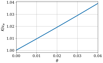
Figure 1 Relative effective momentum dissipation $K/{\mathit{\nu }}_{\mathrm{w}}$, as a function of volumetric ratio of air to water Θ, using Eq. (10). Assumed here, the ratio is $N_{\mathit{\nu }}:={\mathit{\nu }}_{\mathrm{w}}/{\mathit{\nu }}_{\mathrm{a}}=\mathrm{1}/\mathrm{15}$. The range or Θ has been limited to that applicable to oceanic conditions (over the whole range, the relative effective momentum dissipation is a monotonically increasing function).

If we adopt the specific form of χ as in Eq. (10), the dissipation term in Eq. (8) becomes $K{\mathbf{\nabla }}_{\mathbf{R}}^{\mathrm{2}}{\mathit{u}}_{\mathrm{0}}$ when bubbles are present and ${\mathit{\nu }}_{\mathrm{w}}{\mathbf{\nabla }}_{\mathbf{R}}^{\mathrm{2}}{\mathit{u}}_{\mathrm{0}}$, when there are no air bubbles. Equation (10) leads us to conclude that the effective momentum dissipation of water with air bubbles will be different from (actually larger than) ν_w. Physically, there is an increase in the rotational component of the flow and an associated increase in energy dissipation.

3 Air entrainment due to rain

In this section, we assume a statistical distribution for raindrops and derive the consequent density of air bubbles in the ocean surface layer.

3.1 Rain distribution

The density of raindrops is assumed to follow the Marshall–Palmer distribution (see Marshall and Palmer, 1948). The density N_r of raindrops of radius r (meters) per unit volume (“number” m⁻³ m⁻¹) is as follows:

$$\begin{array}{}\text{(11)}& N_r(r,R)=\mathrm{2}{N}_{\mathrm{0}}\exp (-\mathrm{\Lambda }(R\left)r\right),\end{array}$$

where $N_{\mathrm{0}}=\mathrm{8}\times {\mathrm{10}}^{\mathrm{6}}$ m⁻³m⁻¹, $\mathrm{\Lambda }\left(R\right)=\mathrm{8.2}{R}^{-\mathrm{0.21}}\times {\mathrm{10}}^{\mathrm{3}}$ (meter), and R (millimeters per hour) is the rain rate. Using N_r, we can then define the drop rate density (DRD), which describes the rate of falling raindrops of radius r per surface area (“number” m⁻² s⁻¹ m⁻¹). Namely, in the following:

$$\begin{array}{}\text{(12)}& \text{DRD}(r,R)=w_r\left(r\right)N_r(r,R),\end{array}$$

where w_r is the terminal velocity of drops in the air (see Medwin et al., 1992). The terminal velocity is computed following the third-order polynomial estimates of Dingle and Lee (1972).

3.2 Bubble production

To complete our quantitative example, we need to relate the number of bubbles in the upper layer of the ocean to rain. Falling raindrops generate subsurface air bubbles in the neighborhood of the sea surface (see Prosperetti and Oguz, 1993 for a review). Small raindrops produce small air bubbles with a very narrow distribution of radii. Intermediate raindrops, with a radius between 0.55–1.1 mm, were shown not to produce air bubbles (see Medwin et al., 1992). For these, the impinging raindrops do not have the kinetic energy necessary to produce the requisite conical crater and jetting of the sea surface that engulfs air. Large raindrops, with radii larger than 1.1 mm, create a crater and a canopy on the sea surface, which, by collapsing, produces a downward liquid jet at the bottom of the crater, followed by the generation of an air bubble. At high rain rates, the larger raindrops are responsible for the bulk of the gas injection, creating bubbles with a varied distribution of radii.

The production of air bubbles by rain can be measured by acoustic means (see Prosperetti and Oguz, 1993). Oguz and Prosperetti (1990) classify air bubble production by falling raindrops in two regimes. Small raindrops, of radii between 0.41 and 0.55 mm, create type I air bubbles. These have a radius of 0.22 mm and are created at the bottom of a conical crater created on the ocean surface by the impinging raindrop. These air bubbles have a narrow acoustic spectrum with a spectral peak at 14 Hz. The acoustic spectrum for these type I air bubbles was found to be insensitive to the rain rate. Medwin et al. (1990) observed that, when rain hits the ocean surface at an angle, owing to strong winds or very steep wave conditions, the acoustic spectrum peak shifts downward, and there is a broadening of the spectrum at higher frequencies. The type I air bubbles do not contribute significantly to total submerged gas volume, and their contribution will be ignored in what follows.

Raindrops with a radius greater than 1.1 mm produce type II air resonant bubbles of varying radius. The relationship between the raindrop radius r (meters) and the peak acoustic emission frequency f₀ (kilohertz) due to trapped air bubbles was empirically determined (see Medwin et al., 1992) as follows:

$$\begin{array}{}\text{(13)}& f_{\mathrm{0}}={\displaystyle \frac{\mathrm{160}}{\mathrm{8}{r}^{\mathrm{3}}\times {\mathrm{10}}^{\mathrm{9}}}}+\mathrm{0.6}.\end{array}$$

The relation between the near-surface air bubble radius a (meters) and the peak acoustic emission follows from the Rayleigh–Plesset equation (Leighton, 1994, p. 306). For the large bubbles considered here, it can be simplified to Minnaert's formula (see Minnaert, 1933; Plesset and Prosperetti, 1977) as follows:

$$\begin{array}{}\text{(14)}& f_{\mathrm{0}}={\displaystyle \frac{\mathrm{1}}{\mathrm{2}\mathit{\pi }a\times {\mathrm{10}}^{\mathrm{3}}}}\sqrt{{\displaystyle \frac{\mathrm{3}\mathit{\gamma }P}{{\mathit{\rho }}_{\mathrm{0}}}}},\end{array}$$

where γ=1.4 is the ratio of the specific heat of the bubble gas, P is the ambient pressure (surrounding the bubble), and ρ₀=1030 kg m⁻³ is the density of sea water. Close to the surface, the ambient pressure is approximately the surface pressure $P=\mathrm{1.01}\times {\mathrm{10}}^{\mathrm{5}}$ Pa and Eq. (14), further simplified as $f_{\mathrm{0}}=\mathrm{3.25}\times {\mathrm{10}}^{-\mathrm{3}}/a$ (see Medwin and Clay, 1997).

The relation between the entrained air bubble radius a(r) (meters) and the incident raindrop radius r, for large raindrops, thus, reads, for $r>\mathrm{1.1}\times {\mathrm{10}}^{-\mathrm{3}}$ m, as follows:

$$\begin{array}{}\text{(15)}& a\left(r\right)=\mathrm{3.25}\times {\mathrm{10}}^{-\mathrm{3}}{\left({\displaystyle \frac{\mathrm{160}}{\mathrm{8}{r}^{\mathrm{3}}\times {\mathrm{10}}^{\mathrm{9}}}}+\mathrm{0.6}\right)}^{-\mathrm{1}}.\end{array}$$

As an example, raindrops of radius 1.1–2.3 mm produce type II air bubbles of radius 0.2–1.3 mm, respectively.

Small raindrops (r<0.55 mm) almost always produce type I air bubbles. However, this is not the case for larger raindrops. The distribution of the number of air bubbles produced, as a function of the raindrop radius r, was found by Medwin et al. (1992) and is depicted in Fig. 2 as a probability distribution.

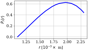
Figure 2 Probability of air bubble creation by large raindrops as a function of raindrop radius r (from Medwin et al., 1992).

3.3 Bubble distribution in the wave boundary layer

Tying back to Sect. 2, by finding the bubble distribution in the wave boundary layer, we can estimate the dimensionless volume fraction Θ. More precisely, the volume fraction reads $\mathrm{\Theta }=\int V\left(a\right)N\left(a\right)\mathrm{d}a$ for bubbles of radius a, with density N(a) (“number” m⁻³ m⁻¹) that occupy a volume $V\left(a\right)=(\mathrm{4}/\mathrm{3})\mathit{\pi }{a}^{\mathrm{3}}$. The aim of the final part of this section is to link Θ to the rain precipitation rate.

In doing so, we will make some approximations. First, bubbles are injected at a very limited depth by raindrops, and this depth may vary with bubble size (see Ho et al., 2000). Second, a homogeneous air bubble distribution in the layer between the depth of injection and the surface is an approximation, as the accumulation of bubbles near the surface can be highly complex due to buoyant forces, damping, and the background turbulence (see, e.g., Merlivat and Memerly, 1983). We will specify how this is taken into account.

The bubble distribution N(a) can be described by an advection–diffusion equation (see Woolf and Thorpe, 1991 and references therein and, for a similar case for oil drops, Moghimi et al., 2018). This equation describes a balance between the advection of bubbles by the vertical fluid velocity, the attenuation of bubble density (i.e., diffusion, which includes the shrinking of bubble radius during their lifetime; see Merlivat and Memerly, 1983), the production of bubbles by rain, and a sink term that captures the loss of air bubbles bursting at the surface or being dispersed by oceanic turbulence.

Solutions of the advection–diffusion equation necessitate the specification of the velocity and the dispersion, generating non-stationary descriptions that might also include mixing due to wave turbulence (see Restrepo et al., 2015; Moghimi et al., 2018).

In the following, the advection–diffusion equation is simplified to estimate the air bubble concentration in a thin layer close to the surface, similar to those in Keeling (1993). First, we assume that the air bubble concentration can be linearly related to a bulk bubble distribution (i.e., averaged over the thin layer), which we, thus, define as c_eN(a). Second, a steady state is considered in which the bulk bubble distribution follows from a balance between the incoming bubble flux due to rain and the outgoing bubble flux due to upward bubble advection and bursting at the surface, as follows:

$$\begin{array}{}\text{(16)}& w_r\left(r\right)P_r\left(r\right)N_r\left(r\right)=c_{e}W\left[a\right(r\left)\right]N\left[a\right(r\left)\right],\end{array}$$

where P_r(r) is the probability of the production of an air bubble by a raindrop of radius r (see Fig. 2), and W(a) is the upward vertical ascent speed of bubbles of radius a. From this equation, the bubble distribution reads $N\left(a\right)=w_r{N}_r(r,R)P_r/\left[c_{e}W\right(a\left)\right]$. We assume, as an estimate for the bubble upward speed W(a), the following form:

$$\begin{array}{}\text{(17)}& W\left(a\right)=\sqrt{{\displaystyle \frac{\mathit{\tau }}{a{\mathit{\rho }}_{\mathrm{0}}}}+ga},\end{array}$$

where $\mathit{\tau }=\mathrm{72.8}\times {\mathrm{10}}^{-\mathrm{3}}$ N m⁻¹ is the air–sea surface tension (see Clift et al., 1978, p. 172). This form, predicted in Mendelson (1967), is valid for ellipsoidal bubbles with a radius greater than 0.65 mm and whose upward path is not rectilinear.

Referring to the above approximations, the factor c_e can first be interpreted as a depth scaling parameter accounting for differences between the bulk estimate and the non-homogeneous bubble distribution N. A further approximation is that the effective vertical velocity of bubbles can be significantly lower than Eq. (17) by up to 60 % due to the presence of contaminants at the bubble surface (see Clift et al., 1978; Fig. 7.3). Hence, the factor c_e is also to be interpreted as a decrease in the bubble vertical velocity, which then reads c_eW(a).

Making use of Eq. (12), $N\left(a\right)=(\text{DRD}\times P_r)\left(r\right)/c_{e}W\left(a\right)$. The volumetric ratio $\mathrm{\Theta }=\int V\left(a\right)N\left(a\right)\mathrm{d}a$, for bubbles of radius a with density N(a) that occupy volume $V\left(a\right)=(\mathrm{4}/\mathrm{3})\mathit{\pi }{a}^{\mathrm{3}}$ then reads as follows:

$$\begin{array}{}\text{(18)}& \mathrm{\Theta }\left(R\right)=\underset{\mathrm{1.1}\times {\mathrm{10}}^{-\mathrm{3}}}{\overset{\mathrm{2.3}\times {\mathrm{10}}^{-\mathrm{3}}}{\int }}{\displaystyle \frac{\mathrm{4}\mathit{\pi }}{\mathrm{3}}}a(r{)}^{\mathrm{3}}{\displaystyle \frac{(\text{DRD}\times P_r)\left(r\right)}{c_{e}W\left(a\right)}}\mathrm{d}r,\end{array}$$

where the limits of integration encompass the volumetric contributions of type II bubbles. The obtained values of volume fraction are consistent with data from the laboratory experiments of Ho et al. (2000) (see their Fig. 7), which suggests that, for rain rates of 114 mm per hour, the volume fraction near the air–water interface is between 10⁻⁶ and 10⁻⁵, corresponding to c_e of the order of 0.1.

4 The effect of rain on gravity and capillary waves

The subject of mathematical models for wave dissipation that reproduce the observed dissipation rates observed in laboratory experiments is considered in the study by Henderson et al. (2015). The focus is on the dissipation effects of small waves due to surface contamination with air above it. Several wave damping models are compared to data. In this work, a model by Jenkins and Jacobs (1997) is compared to experimental data of the damping of small waves. The model posits a small (boundary) layer sitting over a deep water layer. The two-layer model yields expressions valid under several limits. Our work can contribute to this work by defining how the equations in the upper layer are modified by the presence of air bubbles and how their density relates to rain, if this is the mechanism for their generation.

In what follows, we will invoke a far less general, but more consistent, way of addressing the question on how the presence of rain bubbles affects water waves. The derivation of infinitesimal amplitude gravity waves dynamics, starting from Navier–Stokes, appears in Lamb (1926), article 349. We revert to dimensional quantities in what follows. The solution u₀ satisfies the linear version of Eqs. (8) and (9) and the two stress conditions at the surface. Namely, in the following:

$$\begin{array}{}\text{(19)}& {\displaystyle }K\left[{\partial }_X{v}_{\mathrm{0}}+{\partial }_Y{u}_{\mathrm{0}}\right]& {\displaystyle }=\mathrm{0},\text{at}z=\mathit{\eta },\text{(20)}& {\displaystyle }-{\partial }_T{\mathit{\varphi }}_{\mathrm{0}}+\left(g-{\displaystyle \frac{\mathit{\tau }}{{\mathit{\rho }}_{*}}}{\partial }_{XX}\right){\mathit{\eta }}_{\mathrm{0}}+\mathrm{2}K{\partial }_Y{v}_{\mathrm{0}}& {\displaystyle }=\mathrm{0},\text{at}z=\mathit{\eta },\end{array}$$

where ϕ₀ is the mean field velocity potential, and ρ_* is the density of water (no rain) or the reduced density (i.e., raining, with air bubbles in the water), and time (at wave scales) is T. At some distance ℓ below the surface, the conditions are as follows:

$$\begin{array}{}\text{(21)}& {\displaystyle }{\mathit{\nu }}_{\mathrm{w}}[{\partial }_{X}v+{\partial }_{Y}u]=K[{\partial }_X{v}_{\mathrm{0}}+{\partial }_Y{u}_{\mathrm{0}}],\text{at}z=\mathit{\eta }-\mathrm{\ell },\text{(22)}& {\displaystyle }-{\partial }_T\mathit{\varphi }+\mathrm{2}{\mathit{\nu }}_{\mathrm{w}}{\partial }_{Y}v=-{\partial }_T{\mathit{\varphi }}_{\mathrm{0}}+\mathrm{2}K{\partial }_Y{v}_{\mathrm{0}},\text{at}z=\mathit{\eta }-\mathrm{\ell }.\end{array}$$

By combining the boundary and non-boundary solutions, the approximate solution of the system, assuming a vanishingly small upper layer thickness and vanishing velocity at depth, is as follows:

$$\begin{array}{}\text{(23)}& \begin{array}{rl}& \mathit{\varphi }=A{e}^{kZ+i(kX-\mathit{\sigma }T)}\exp [-\mathrm{2}K{k}^{\mathrm{2}}T],\\ & \mathit{\psi }={\displaystyle \frac{\mathrm{2}K{k}^{\mathrm{2}}A}{\mathit{\sigma }}}{e}^{kZ+i(kX-\mathit{\sigma }T)}\exp [-\mathrm{2}K{k}^{\mathrm{2}}T],\\ & \mathit{\eta }={\displaystyle \frac{kA}{\mathit{\sigma }}}{e}^{i(kX-\mathit{\sigma }T)}\exp [-\mathrm{2}K{k}^{\mathrm{2}}T],\end{array}\end{array}$$

where ψ is the streamfunction, and σ is the angular frequency. The solution (23) represents infinitesimal progressive waves traveling in the X direction.

The dispersion relation for the waves is as follows:

$${\mathit{\sigma }}^{\mathrm{2}}=gk+{\displaystyle \frac{\mathit{\tau }}{{\mathit{\rho }}_{*}}}{k}^{\mathrm{3}},$$

showing that changes in the surface tension due to the presence of air bubbles injected by the rain impacts the dispersion relation. The effective density is as follows:

$${\mathit{\rho }}^{*}={\displaystyle \frac{\mathrm{1}}{\mathrm{\Omega }}}\underset{\mathrm{\Omega }}{\int }\mathit{\rho }\left(\mathit{r}\right)\mathrm{d}\mathit{r},$$

which, in our simplified accounting, would be ${\mathit{\rho }}^{*}=\mathrm{\Theta }{\mathit{\rho }}_{\mathrm{a}}+(\mathrm{1}-\mathrm{\Theta }){\mathit{\rho }}_{\mathrm{w}}$.

The effective wave dissipation 2K appears in the exponential factor exp [−2Kk²T]. When the rainstorm is sufficiently intense (but the raindrops are not too large), the wave dissipation 2K will change from 2ν_w to a higher value, depending on how much air is injected by the impinging raindrops.

The dependence of the effective wave dissipation on the rain rate, using Eqs. (10) and (18), is depicted in Fig. 3. The surface tension effect increases as well, affecting the dispersion relation. These effects are manifest primarily in capillary, high-frequency wave components. The bubble model derived in Sect. 3 has one free parameter, c_e, which controls the upward flux of bubbles. The solid line shows the wave dissipation for c_e=1, i.e., the situation for which the bulk estimation of the upward flux of bubbles is assumed to be correct. The dashed line shows the wave dissipation corresponding to the more realistic value, c_e=0.1, which matches the measured volume fraction of Ho et al. (2000). With respect to c_e=1, it corresponds to a situation where the residence time of the bubbles in the upper ocean layer is increased, due to, e.g., near-surface turbulence.

In both cases, the increase in effective wave damping due to the injection of air, at least as estimated by simple considerations, is small compared to the values reported in the experiments in Peirson et al. (2013) (and in Tsimplis, 1992), further proof of what was stated in the introduction – i.e., that, for large rain rates and, as in the wave tank experiments, large raindrops, the mechanical effect is dominant for the immediate, albeit limited, attenuation of water waves. In these instances, using very high rain rates, the effective dissipation was found to increase by 3–10 times when rain is present, compared to without rain.

Figure 3 also shows the sensitivity of the model to changes in ${\mathit{\nu }}_{\mathrm{w}}/{\mathit{\nu }}_{\mathrm{a}}$, which is much lower than to changes in the bubbles volume fraction, i.e., the tuning parameter c_e. The gray shading shows the intervals obtained by varying the air viscosity inside air bubbles (ν_a) from 10⁻⁵ to 10⁻⁴ (the lower and upper parts of the shading, respectively) for a fixed c_e of 0.1. This range of variation in ν_a corresponds to variations in the effective kinematic viscosity of air due to the mechanical effect of raindrops, as observed in Harrison and Veron (2017).

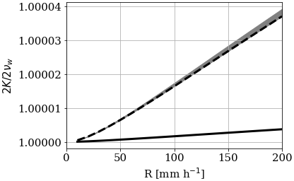
Figure 3 Relative effective wave dissipation $\mathrm{2}K/\mathrm{2}{\mathit{\nu }}_{\mathrm{w}}$, as a function of rain rate R for two values of the unconstrained parameter, c_e, with 1 (solid) and 0.1 (dashed). The very small region with the gray shading, below the upper curve, corresponds to a variation in air diffusivity between 10⁻⁵ m s⁻² (dashed line) and 10⁻⁴ m s⁻² for a fixed c_e=0.1. The figure highlights that the model outcomes are more sensitive to the parameter c_e than to the value of the diffusivity ν_a.

5 Discussion and conclusions

Stimulated by an oceanographic problem, we have developed a physical–mathematical approach to analyze how the presence of a large number of small bubbles affects the characteristics of the containing liquid. Given the general method and having specified the necessary conditions for its application, we focused on a specific example, namely the presence of air bubbles in the thin upper layer of the ocean, and their impact on ocean surface waves. We first derived the (upscaled) equations for mass and momentum conservation. The upscaled velocity and pressure are averages over sub-wave scales over which the material with heterogeneities assumes a stationary distribution. These equations revealed that the effective (upscaled) momentum dissipation is increased when bubbles are present with respect to the no-bubble case.

Under homogenization conditions, the model yields a dynamic equation that has a higher effective diffusion constant with bubbles than without bubbles. This translates into an increased kinematic viscosity of the air–water mixture, which is directly related to an increase in the damping of surface waves. The source for the tiny uniformly distributed bubbles is, in our case, rain, whose small drops generate the bubble distribution (large drops lead to splashing and turbulence in the upper layer, which is a different process). For typical rain rates, we found that the resulting wave damping due to bubbles is not significant with respect to other damping sources, such as turbulence-induced dissipation due to the impact of large raindrops. We also found that the presence of bubbles affects the capillary waves' dispersion relation through a change in the effective surface tension felt by the waves.

The increase in wave damping (related to kinematic viscosity) when bubbles are present may appear counterintuitive at first sight, but it results from kinematic viscosity being the ratio of the dynamic viscosity and the density of the fluid of interest. As bubbles are injected into water, the homogenized kinematic viscosity decreases, but so does the homogenized fluid density, with the overall effect being an increase in the homogenized kinematic viscosity. Physically, the presence of small bubbles at the typically small void ratios of non-breaking waves enhances the momentum transfer between the waves and the mean flow. The enhanced wave rotational component results in higher viscous effects. Moreover, since the density enters explicitly in the definition of the surface tension force, when the volume fraction of air to water is not zero, then the average density of the medium decreases, and, thus, with this decrease comes an increase in surface tension forces. Finally, the viscous effects and changes in the surface tension also lead to changes in the dispersion relation and, as a consequence, in the wave group velocity as well.

Many simplifications were made in the formulation of the rain/wave model. In the momentum equation, we used the most simplistic model for the tensor D(r); the consequence is meek momentum exchanges between the rotational and irrotational components of the velocity, and this argues for a more vigorous research effort in determining more realistic models for the tensor. In particular, the tensor should account for all sources of small-scale heterogeneity besides air bubbles. The model for the mechanism that ties the rain, the bubble presence in the layer, and the momentum and mass conservation equations below the free surface has three critical parameters, namely the rain rate R, the air-to-water volume fraction Θ (through the flux strength parameter, c_e, associated with the upward flux of air bubbles from their injection depth to the surface), and the ratio of diffusivities of water and air, N_ν. Given those approximations, the basic result is that the volume fraction of air to water would have to be exceptionally large for the effect to be significant when compared to other damping mechanisms. However, granted the limited effect in the analyzed case, larger amounts of bubbles or, mutatis mutandis, of buoyant organic or hydrocarbons are certainly possible. In these cases that we have not explored, the damping effect can indeed be relevant and, within the specified approximations, quantifiable following the procedure we have outlined.

A last simplification is related to the fact that waves occur in a salty ocean. The densities of the fresh water due to rain and the salt water of the ocean are different. Both fresh water and air bubbles are, thus, affecting the composition of the ocean in the near surface and, thus, the local density and the tensor D(r). The change in the water composition will also affect some aspects of the bubble distribution model presented earlier. The more complex composition will quantitatively affect the results, but it is presumed not to affect the qualitative conclusions presented. Another effect that has been ignored here is a full consideration of the water–air interface stress conditions when rain is present. In Veron and Meussiens (2016), a model is presented for how the impact of rain affects the boundary conditions (see their Eqs. 2.11, 2.14, and, for waves, 3.4), i.e., the pressure at the free surface is composed of the atmospheric pressure plus a rain-induced pressure. The rain-induced pressure is trivially space averaged in order to enter the homogenized set of momentum/condition equations presented here. The consequences on the waves enter through Bernoulli's equation and affect the dispersion of the waves. These issues are presented in Veron and Meussiens (2016) and not repeated here.

There are several processes in which the mixture of a liquid containing a large number of bubbles or droplets has different characteristics. Examples are a frothy ocean, whatever the content, or cavitating flows, as it happens in ship propellers or in pressurized flows. An example we came across while preparing this article describes how foams are used to ameliorate unwanted ship motion due to sloshing of their holding tank contents (see Denkov et al., 2005; Kim et al., 2007) and the stabilizing effect of free surface sloshing of bubbly drinks (see Sauret et al., 2015). These foamy cases are non-trivial extensions of the homogenization procedure we present in this paper. Consideration of the chemistry, compressible effects, and topology is required, and the intricate formulation of the stress conditions at the interfaces would need to be derived. Nevertheless, the procedure may play a constructive role in formulating a mean field description of the dissipation and the consequent attenuation of the foam on sloshing motions.

6 Summary

We itemize our main conclusions here, as follows:

1. A general methodology has been developed to quantify the effect of small-scale bubbles on the properties of the containing liquid. Averaged dynamic quantities can be defined, and for these, averaged momentum and mass conservation equations of general applicability can be derived.

2. A model was derived that permits an estimate of the amount of air injected by rain.

3. The presence of tiny air bubbles, which we assume are uniformly distributed, changes the physical characteristics of the containing liquid, affecting the momentum balances – the momentum dissipation of irrotational motions is enhanced due to an increase in the rotational component of the flow.

4. We have also specifically addressed the impact of the presence of air bubbles on gravity waves. We found that air bubbles increase the effective wave damping and, hence, that rain has a damping effect on waves. Changes in the density near the free surface will also affect the surface tension. Since the generation of bubbles by rain is small in the natural setting, the damping effect is small, akin to the damping of waves due to surface contamination. An increase in wave damping has implications for momentum exchanges between the waves and the mean flow. Wave damping changes and surface tension changes impact the wave dispersion relation and the group velocity. These effects are primarily relevant to the dynamics of small and capillary waves.

5. We have cited a number of situations where, granted certain conditions, our approach can be applied for a general estimate of the overall increased dissipation.