Enhanced internal tidal mixing in the Philippine Sea mesoscale environment

Turbulent mixing in the ocean interior is mainly attributed to internal wave breaking; however, the mixing properties and the modulation effects of mesoscale environmental factors are not well known. Here, the spatially inhomogeneous and seasonally variable diapycnal diffusivities in the upper Philippine Sea were estimated from Argo float data using a strain-based, fine-scale parameterization. Based on a coordinated analysis of multi-source data, we found that the driving processes for diapycnal diffusivities mainly included the near-inertial waves and internal tides. Mesoscale features were important in intensifying the mixing and modulating of its spatial pattern. An interesting finding was that, besides near-inertial waves, internal tides also contributed significant diapycnal mixing in the upper Philippine Sea. The seasonal cycles of diapycnal diffusivities and their contributors differed zonally. In the midlatitudes, wind mixing dominated and was strongest in winter and weakest in summer. In contrast, tidal mixing was more predominant in the lower latitudes and had no apparent seasonal variability. Furthermore, we provide evidence that the mesoscale environment in the Philippine Sea played a significant role in regulating the intensity and shaping the spatial inhomogeneity of the internal tidal mixing. The magnitudes of internal tidal mixing were greatly elevated in regions of energetic mesoscale processes. Anticyclonic mesoscale features were found to enhance diapycnal mixing more significantly than cyclonic ones.

1 Introduction

Turbulent mixing can alter both the horizontal and vertical distributions of temperature and salinity gradients. These then modulate the ocean circulation variability, both globally and regionally. Many studies have shown the existence of a complicated spatiotemporal pattern of diapycnal mixing in the ocean interior. Such mixing inhomogeneity can influence the hydrological characteristics, ocean circulation variability, and climate change. The breaking of internal waves is believed to be the main contributor to the ocean's diapycnal mixing (e.g., Liu et al., 2013; Robertson, 2001). Thus, a clear understanding of the spatial patterns and dissipation processes of broadband internal waves is necessary to clarify and depict the global ocean mixing climatology.

The long-wavelength internal waves in the ocean occur mainly in the form of near-inertial internal waves (NIWs) and internal tides (e.g., Alford and Gregg, 2001; Cao et al., 2018; Klymak et al., 2006; Xu et al., 2013), and the internal solitary waves evolved from them also can trigger mixing (e.g., Deepwell et al., 2017; Grimshaw et al., 2010; Shen et al., 2020). The wind-input NIW energy to the mixing layer is about 0.3–1.4 TW (e.g., Alford, 2003; Liu et al., 2017; Rimac et al., 2013; Watanabe and Hibiya, 2002). The NIW energy propagates downward, mainly dissipating, and drives energetic mixing within the upper ocean (Wunsch and Ferrari, 2004). Barotropic tidal currents flowing over rough topographic features can generate internal tides (e.g., Robertson, 2001; Xu et al., 2016), with the global energy of 1.0 TW (Egbert and Ray, 2001; Jayne and St. Laurent, 2001; Song and Chen, 2020). Near the generation sources, internal tidal mixing intensifies above the bathymetries; meanwhile, in remote areas, the tidal mixing becomes distributed throughout the water column due to the multiple reflection and refraction processes. Therefore, the relative contributions to the upper-layer diapycnal diffusivities by NIWs and the spatial variability in internal tides deserve further investigation.

In the midlatitudes, NIWs dominate the upper ocean mixing as a result of the presence of westerlies and frequent storms (e.g., Alford et al., 2016; Jing et al., 2011; Whalen et al., 2018). However, from the global view, the upper ocean mixing geography is inconsistent with the global wind field distribution. For example, in low latitudes, upper ocean mixing hotspots are located nearer to rough topographic features, regardless of the wind conditions. This indicates that upper ocean mixing might be attributed to non-wind-driven internal waves, such as internal tides. In order to better understand the ocean mixing patterns and modulation mechanisms, we need to clarify the relative contributions between the wind and tidal energy.

Internal tides are generally considered to be important to ocean mixing in the deep ocean, below the influence of winds (Ferrari and Wunsch, 2009; Munk and Wunsch, 1998; MacKinnon et al., 2017). Many factors influence the spatial pattern and energy transfer of internal tides. Higher-mode internal tides break more easily near their sources, while the low-mode internal tides propagate long distances, even thousands of kilometers. Propagating internal tides will be limited by several factors, such as topography, stratification, and turning latitude (e.g., Vlasenko et al., 2013; Song and Chen, 2020; Hazewinkel and Winters, 2011). Wave–wave interaction in the ocean also influences the spatiotemporal variability of internal tides. For example, PSI (parametric subharmonic instability) is a potential avenue for transferring internal tidal energy to other frequencies (Ansong et al., 2018). Moreover, stratification and background flows also contribute to internal tidal spatial and temporal variability (e.g., Kerry et al., 2016; Huang et al., 2018; Tanaka et al., 2019; Chang et al., 2019). Due to the complicated multi-scales of the background flows, it is still unclear how the background flow modulates the internal tides, their energy dissipation, and ocean mixing.

Recent research suggests that the mesoscale environment is a key factor influencing ocean mixing. There is evidence that mesoscale eddies can enhance wind-driven mixing and internal tidal dissipation. This enhancement will be more significant in the presence of an anticyclonic eddy (e.g., Jing et al., 2011; Whalen et al., 2018). Similarly, regional studies indicate that mesoscale features modulate the generation and propagation of internal tides. Mesoscale currents can also broaden the range undergoing internal tide critical latitude effects and enhance the energy transfer from diurnal frequencies to semidiurnal or high frequencies (Dong et al., 2019). Mesoscale eddies are found to modulate internal tide propagation (Rainville and Pinkel, 2006; Park and Watts, 2006; Zhao et al., 2010) and enable the internal tide to lose its coherence (Nash et al., 2012; Kerry et al., 2016; Ponte and Klein, 2015). Numerical simulation results support these observations (Kerry et al., 2014), indicating that the patterns of internal tides are largely modulated by the position of eddies. An idealized numerical experiment shows that the energy of internal tides shows bundled beams after passing through an eddy (Dunphy and Lamb, 2014). And the mode-1 internal tidal interactions with eddies will trigger higher-mode signals. Up to now, research on mesoscale–internal tide interactions has been primarily focused on the propagation pattern or 3-D structure of internal tides and has ignored their energy dissipation and mixing effects. The latter are more important for impacts on the ocean circulation variability and climate change.

The Philippine Sea, located in the northwestern Pacific Ocean, is one of the most energetic internal tidal regimes in the world. In this region, powerful internal tides significantly enhance ocean mixing, as shown by numerical simulations (Wang et al., 2018). The importance of sub-inertial shear to ocean mixing has been hypothesized from observations (Zhang et al., 2018), and the importance of internal tides to mixing is supported through parameterization techniques (Qiu et al., 2012). On the other hand, the Philippine Sea is an area with frequent typhoons, which make significant contributions to ocean mixing. Consequently, multiple factors and mechanisms impact the turbulent mixing distribution in the Philippine Sea (Wang et al., 2018). To date, it is unclear what the dominant factors are and how these factors modulate the ocean mixing properties. Moreover, the role of the mesoscale environment in regulating ocean mixing is still not well understood.

Presently, coupled numerical models are basically able to accurately simulate the generation and propagation of internal tides. The internal tide dissipation and induced mixing are found to be important for the determination of correct mixing parameterizations in numerical models (Robertson and Dong, 2019). Some existing studies focus on the simulations of internal tidal breaking and tidally induced mixing (Kerry et al., 2013, 2014; Muller, 2013; Wang et al., 2018). It is difficult to provide a complete spatial and temporal picture from direct observations of turbulence. This is due to the scarcity of observations and their patchy distribution in time and space. Multisource data covering multiple tidal cycles, or preferably a spring neap cycle, and a broad domain are necessary to acquire the spatiotemporal distribution, and very little of these data have been collected. The development and application of parameterization methods provide a greater possibility of characterizing a broad regional mixing distribution and variability. A global pattern of ocean mixing has been provided using these parameterization methods (Whalen et al., 2012; Kunze, 2017). Furthermore, sensitivity studies have been performed investigating the dependence of several factors to global mixing, such as bottom roughness, internal tides, wind, and background flows (e.g., Whalen et al., 2012; Waterhouse et al., 2014; Kunze, 2017; Whalen et al., 2018; Zhang et al., 2018). At present, parameterization is the most effective method for investigating the modulation of tidal mixing by mesoscale background flows.

The spatial pattern and temporal variability in diapycnal diffusivities in the Philippine Sea are examined in this paper. We provide evidence to verify the importance of tidal mixing in the upper layer of this region. Moreover, we illustrate the modulation of the mesoscale environment in tidal mixing properties and distributions. Our data and methods are detailed in Sect. 2. Results and analysis, including the spatial patterns and seasonal cycle of mixing, contributions of influencing factors, and internal tide–mesoscale interrelationships, are found in Sect. 3. Finally the summary and discussion are given in Sect. 4.

2 Method and data

2.1 Argo and fine-scale parameterization method

The Argo program is a joint international effort involving more than 30 countries and organizations and having deployed over 15 000 freely drifting floats since 2000. The accumulated total of collected profiles exceeds 2 million profiles of conductivity, temperature, and depth (CTD) along with other geobiochemical parameters. The Argo program has become the main data source for many research and operational predictions of oceanography and atmospheric science (http://www.ARGO.ucsd.edu, last access: 8 May 2021). We screened the profiles from the Philippines Sea with quality control and estimated diapycnal diffusivity and dissipation rates from them using a fine-scale parameterization.

The diapycnal diffusivity and turbulent kinetic energy dissipation rate can be estimated from a fine-scale strain structure. This is based on a hypothesis that the energy can be transported from large to small scales. In such scales, waves break due to shear or convective instabilities by weakly nonlinear interactions between internal waves (Kunze et al., 2006). Presently, this method has been widely used for the global ocean (e.g., Wu et al., 2011; Kunze, 2017; Whalen et al., 2012; Fer et al., 2010; Waterhouse et al., 2014). The dissipation rate ε can be expressed as follows:

$$\begin{array}{}\text{(1)}& \mathit{\epsilon }={\mathit{\epsilon }}_{\mathrm{0}}{\displaystyle \frac{\stackrel{\mathrm{‾}}{N^{\mathrm{2}}}}{N_{\mathrm{0}}^{\mathrm{2}}}}{\displaystyle \frac{\langle {\mathit{\xi }}_z^{\mathrm{2}}{\rangle }^{\mathrm{2}}}{\langle {{\mathit{\xi }}_z^{\mathrm{2}}}_{\mathrm{GM}}{\rangle }^{\mathrm{2}}}}h\left(R_{\mathit{\omega }}\right)L\left(f,\stackrel{\mathrm{‾}}{N}\right),\end{array}$$

where ${\mathit{\epsilon }}_{\mathrm{0}}=\mathrm{6.73}\times {\mathrm{10}}^{-\mathrm{10}}$ W kg⁻¹, $N_{\mathrm{0}}=\mathrm{5.24}\times {\mathrm{10}}^{-\mathrm{3}}$ s⁻¹, and $\stackrel{\mathrm{‾}}{N^{\mathrm{2}}}$ represents the averaged buoyancy frequency of the segment. $\langle {{\mathit{\xi }}_z^{\mathrm{2}}}_{\mathrm{GM}}\rangle$ and $\langle {\mathit{\xi }}_z^{\mathrm{2}}\rangle$ are strain variance from the Garrett–Munk (GM) spectrum (Gregg and Kunze, 1991) and the observed strain variance, respectively. The angle brackets indicate integration over a specified range of vertical internal wavenumbers (see Eqs. 4 and 5). The function h(R_ω) accounts for the frequency content of the internal wave field, and R_ω represents shear and strain variance ratio. R_ω is fixed at 7, which is a global mean value (Kunze et al., 2006).

$$\begin{array}{}\text{(2)}& h\left(R_{\mathit{\omega }}\right)={\displaystyle \frac{\mathrm{1}}{\mathrm{6}\sqrt{\mathrm{2}}}}{\displaystyle \frac{R_{\mathit{\omega }}\left(R_{\mathit{\omega }}+\mathrm{1}\right)}{\sqrt{R_{\mathit{\omega }}-\mathrm{1}}}}.\end{array}$$

The function $L\left(f,\stackrel{\mathrm{‾}}{N}\right)$ corrects for a latitudinal dependence; here, f is the local Coriolis frequency, so f₃₀ is the Coriolis frequency at 30^∘, and $\stackrel{\mathrm{‾}}{N}$ is the vertically averaged buoyancy frequency of the segment.

$$\begin{array}{}\text{(3)}& L\left(f,\stackrel{\mathrm{‾}}{N}\right)={\displaystyle \frac{f\mathrm{arccosh}\left(\frac{\stackrel{\mathrm{‾}}{N}}{f}\right)}{f_{\mathrm{30}}\mathrm{arccosh}\left(\frac{\stackrel{\mathrm{‾}}{N}}{f_{\mathrm{30}}}\right)}}.\end{array}$$

Strain ξ_z was calculated from each segment as follows:

$$\begin{array}{}\text{(4)}& {\displaystyle }{\mathit{\xi }}_z={\displaystyle \frac{N^{\mathrm{2}}-N_{\mathrm{ref}}^{\mathrm{2}}}{\stackrel{\mathrm{‾}}{N^{\mathrm{2}}}}}\text{(5)}& {\displaystyle }\langle {\mathit{\xi }}_z^{\mathrm{2}}\rangle ={\int }_{k_{\min }}^{k_{\max }}{S}_{\mathrm{str}}\left(k_z\right)\mathrm{d}{k}_z\le \mathrm{0.2}.\end{array}$$

We derived N from 2 to 10 dbar processed temperature, salinity, and pressure data according to the Argo float resolution. N_ref, as a smooth, piece-wise quadratic fit to the observed N profile, is fitted to 24 m. Here we remove segments that vary in the range of $\langle N^{\mathrm{2}}\rangle >\mathrm{5}\times {\mathrm{10}}^{-\mathrm{4}}$ s⁻² or $\langle N^{\mathrm{2}}\rangle <\mathrm{1}\times {\mathrm{10}}^{-\mathrm{9}}$ s⁻², since the strain signal at these levels is dominated by noise (Whalen et al., 2018). By applying a fast Fourier transform (FFT) on half-overlapping 256 m segments along each vertical ξ_z profile, we computed the spectra S_str(k_z) and integrated them to determine the strain variance. We integrated these spectra between the vertical wavenumbers k_min=0.003 cpm and k_max=0.02 cpm, according to typical global internal tidal scales and Eq. (5), respectively. Substituting $\langle {\mathit{\xi }}_z^{\mathrm{2}}\rangle$ into Eq. (1) ultimately yields 32 m resolved vertical sections of each observed profile. The dissipation rate ε is related to the diapycnal diffusivity K_z by the Osborn relation as follows:

$$\begin{array}{}\text{(6)}& K_z=\mathrm{\Gamma }{\displaystyle \frac{\mathit{\epsilon }}{\stackrel{\mathrm{‾}}{N^{\mathrm{2}}}}},\end{array}$$

where the flux coefficient Γ is fixed at 0.2 generally.

2.2 ERA-Interim and slab model

The near-inertial energy flux for each observation profile was calculated using the 10 m wind speed product from ERA-Interim (https://www.ecmwf.int/en/forecasts/datasets, last access: 8 May 2021), which is a 6 h wind speed on a grid of 0.75^∘ × 0.75^∘. We selected the mean near-inertial flux of 30–50 d before the time of each diapycnal diffusivity estimation as our measure of the near-inertial flux, with the consideration of the propagation of NIWs.

The wind-driven NIW energy flux can be directly estimated using a slab model, which assumes that the inertial oscillations in the mixed layer do not interact with the background fields. The mixed layer current velocity can be described by the following:

$$\begin{array}{}\text{(7)}& {\displaystyle \frac{\mathrm{d}Z}{\mathrm{d}t}}+\left(r+if\right)Z={\displaystyle \frac{T}{\mathit{\rho }H}},\end{array}$$

where $Z=u+iv$ is the mixed layer oscillating component of full current, and i is an imaginary number to indicate the latitudinal component. $\mathrm{T}=\left({\mathit{\tau }}_x+i{\mathit{\tau }}_y\right)$ is the wind stress on the sea surface, f is the local Coriolis parameter, and r is the frequency-dependent damping parameter, which was fixed at 0.15f for these calculations. ρ is sea water density and fixed at 1024 kg m⁻³. H is the mixed-layer depth and was set to a constant 25 m. We can calculate the oscillating component of the full velocity from Eq. (7) and obtain the near-inertial component through a bandpass filter of [0.85,1.25]f. The near-inertial energy flux is calculated as follows:

$$\begin{array}{}\text{(8)}& E\left(\mathrm{\Pi }\right)=Re\left(Z\cdot T^{\ast }\right).\end{array}$$

The asterisk (^*) indicates the complex conjugate of a variable.

2.3 Aviso+ and eddy kinetic energy (EKE)

The eddy kinetic energy (EKE) is estimated based on geostrophic calculation as follows:

$$\begin{array}{}\text{(9)}& {\displaystyle }\mathrm{EKE}={\displaystyle \frac{\mathrm{1}}{\mathrm{2}}}\left({U_{\mathrm{g}}^{\prime }}^{\mathrm{2}}+{V_{\mathrm{g}}^{\prime }}^{\mathrm{2}}\right)\text{(10)}& {\displaystyle }{U}_{\mathrm{g}}^{\prime }=-{\displaystyle \frac{g}{f}}{\displaystyle \frac{\mathrm{\Delta }{\mathit{\eta }}^{\prime }}{\mathrm{\Delta }y}}{V}_{\mathrm{g}}^{\prime }=-{\displaystyle \frac{g}{f}}{\displaystyle \frac{\mathrm{\Delta }{\mathit{\eta }}^{\prime }}{\mathrm{\Delta }x}},\end{array}$$

where $U_{\mathrm{g}}^{\prime }$ and $V_{\mathrm{g}}^{\prime }$ are the geostrophic velocities in the east–west and north–south directions, respectively. They are taken from the Aviso+ (http://www.aviso.altimetry.fr/duacs/, last access: 8 May 2021) geostrophic velocity product. η^′ indicates the sea level anomaly (SLA).

2.4 Internal tidal conversion rates

The internal tidal conversion rate was provided by SEANOE (SEA scieNtific Open data Edition; https://www.seanoe.org/recordview, last access: 8 May 2021, Falahat et al., 2018), including eight main tidal constituents. We used the mode-summed internal tidal conversion rates of M₂ and K₁, and integrated eight main tidal constituents in the present study.

3 Results

3.1 Spatial pattern of diapycnal mixing in the upper Philippine Sea

The diapycnal diffusivities were used as indicators of ocean diapycnal mixing. The pattern averaged within 250–500 m is shown in Fig. 1a. The K_z was estimated from the Argo profiles, with an average on each cell of 0.5^∘ × 0.5^∘. The magnitude of diapycnal diffusivities increased with latitude, reaching 10⁻⁴ m² s⁻¹ in the northern part of this area (30–36^∘ N). The mean value of K_z was about O(−6)–O(−5) at lower latitudes, while it was remarkable that the magnitude of K_z also increased significantly in some low-latitude regions, reaching O(−4) or higher, such as in the Luzon Strait (Xu et al., 2014). Reviewing the influence of topography, wind, and internal tides (Fig. 1b–d) on ocean mixing, it was found that the latitudinal variability in K_z was consistent with the wind intensity distribution. Upper ocean mixing was significantly enhanced at midlatitudes due to the presence of westerlies. In addition, K_z was also enhanced near several key internal tide sources, such as the Luzon Strait and Bonin, Izu, and Dadong ridges, etc. At these sites, the magnitude of K_z was obviously larger than other areas at the same latitude, indicating a significant role of internal tides. Additionally, the enhancement of deep ocean mixing at these sites was even more obvious (not shown).

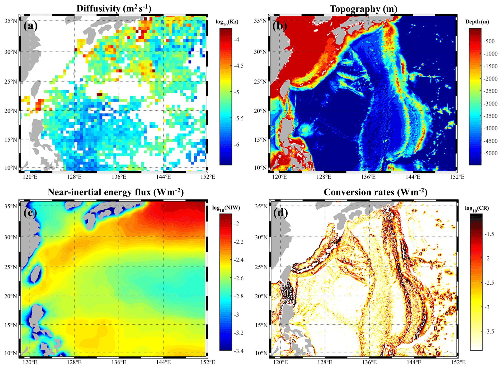
Figure 1 Maps of (a) log-scale averaged diapycnal diffusivities K_z (square meters per second – m² s⁻¹) estimated from Argo profiles. (b) Topography, (c) log-scale, long-term averaged near-inertial energy flux from wind (watts per square meter – W m⁻²), and (d) log-scale M₂ internal tide conversion rates (watts per square meter – W m⁻²).

It can be noted that the pattern of diapycnal diffusivities was not completely consistent with those of either internal tides or winds. This suggests that the ocean mixing was modulated by factors other than tides and winds. The magnitudes of K_z also vary for internal tide source sites. Considering that the Philippine Sea is a region with energetic mesoscale motions (Fig. 2), the influences of mesoscale features in turbulent mixing should be taken into account. The existence of mesoscale features can alter the propagation and dissipation of internal tides. Therefore, the Philippine Sea is an ideal region for studying the modulation of background flows on turbulent mixing associated with strong internal tides.

Figure 2 Maps of (a) log-scale, long-term averaged EKE and (b) long-term averaged vorticity.

3.2 Seasonal variability in mixing at different latitudes

The seasonal cycle for diapycnal diffusivities also differs zonally. Here, we divided the Philippine Sea into two portions, i.e., low latitude (10–25^∘ N) and midlatitude (25–35^∘ N). The diapycnal diffusivities K_z were averaged in each latitude band (Fig. 3). At the depth of 250–500 m in the midlatitude, the diapycnal diffusivities had a significant seasonal trend that was strong in winter and weak in summer. This is consistent with the seasonal fluctuation of near-inertial energy from wind. Such a seasonal cycle could also be found at 500–1000 and 1000–1500 m in the midlatitudes, but it was relatively weaker, especially after 2016. In the lower latitudes, the NIW energy was still strong in winter and weak in summer, but a seasonal dependence of turbulent mixing was not obvious, even in the upper ocean. Consequently, the wind was found to play a significant role in driving turbulent mixing at midlatitudes but was insignificant at low latitudes. Other factors drove and modulated turbulent mixing in low latitudes.

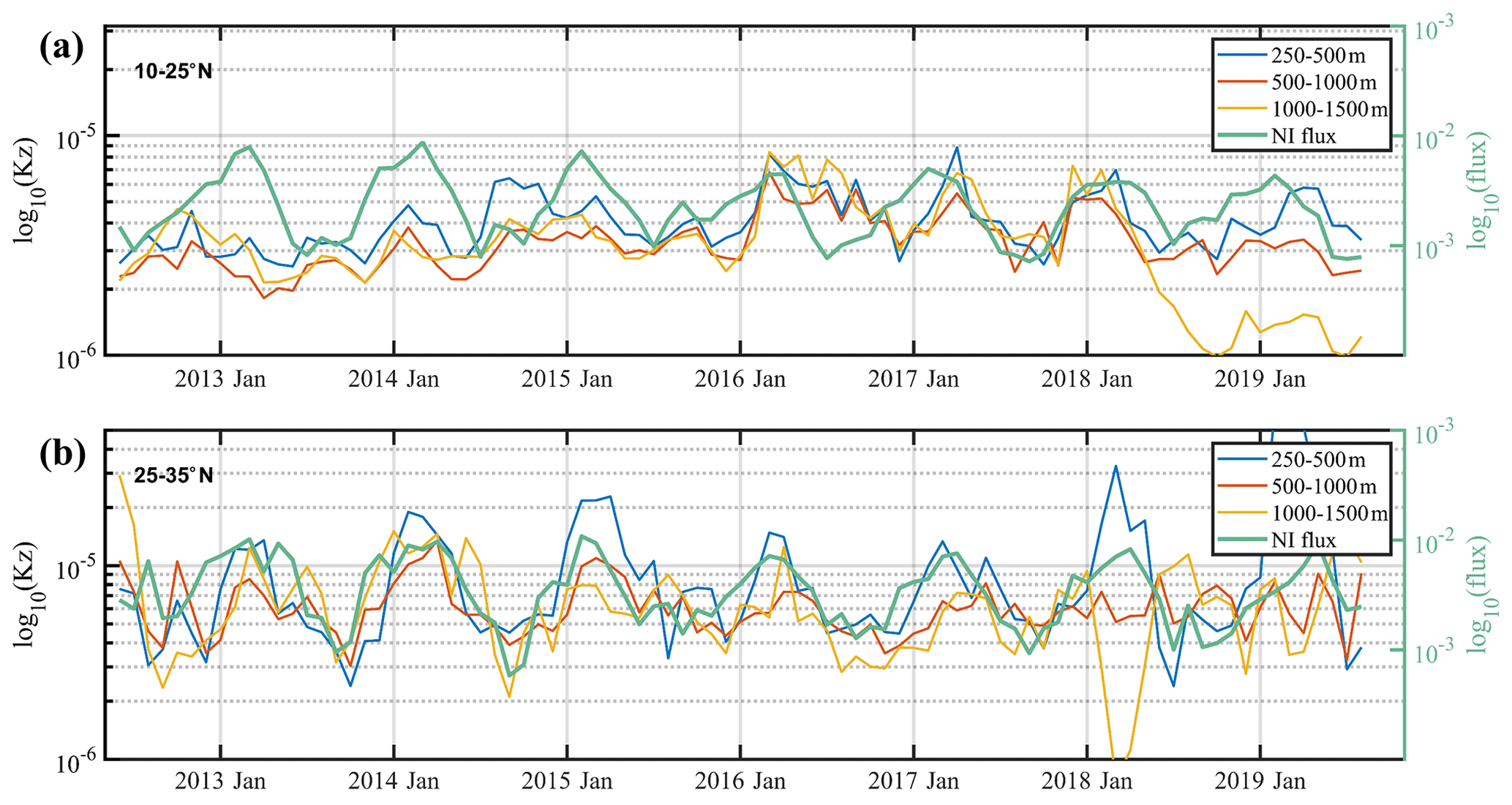
Figure 3 Seasonal cycles in diapycnal diffusivities (colorful lines) and near-inertial energy flux from wind (green) extents at 250–500, 500–1000, and 1000–1500 m in (a) 10–25^∘ N and (b) 25–35^∘ N, which is averaged in each month and in all water columns.

3.3 Impact factors

3.3.1 Relative contributions

The turbulent mixing of the Philippine Sea displayed an obvious latitudinal dependence, so the latitudinal influence was examined for several factors, i.e., internal tides, wind, and EKE (Fig. 4). Each 1^∘ latitude band was separated into two regions with weak or strong internal tides (or other factors). Here we define the strong or weak internal tides as the internal tide conversion rate, which is larger or smaller than the median of the Philippine Sea. The diapycnal diffusivities in these two kinds of regions were then averaged. A similar method has been used to analyze the effect of topography and different frequency bands in internal waves on ocean interior shear and mixing (e.g., Whalen et al., 2012; Zhang et al., 2019). For a more direct representation, the ratios of diapycnal diffusivities above the strong internal tides to weak internal tides were shown. A ratio larger than 1 means that the diapycnal diffusivities are significantly higher in the regions of strong internal tides. The larger this ratio is, the more important the internal tidal induced mixing. Similarly, the contributions of near-inertial wave and EKE were analyzed by this statistical method. The strong near-inertial wave or EKE is defined as being the locations where this parameter exceeds the regional median.

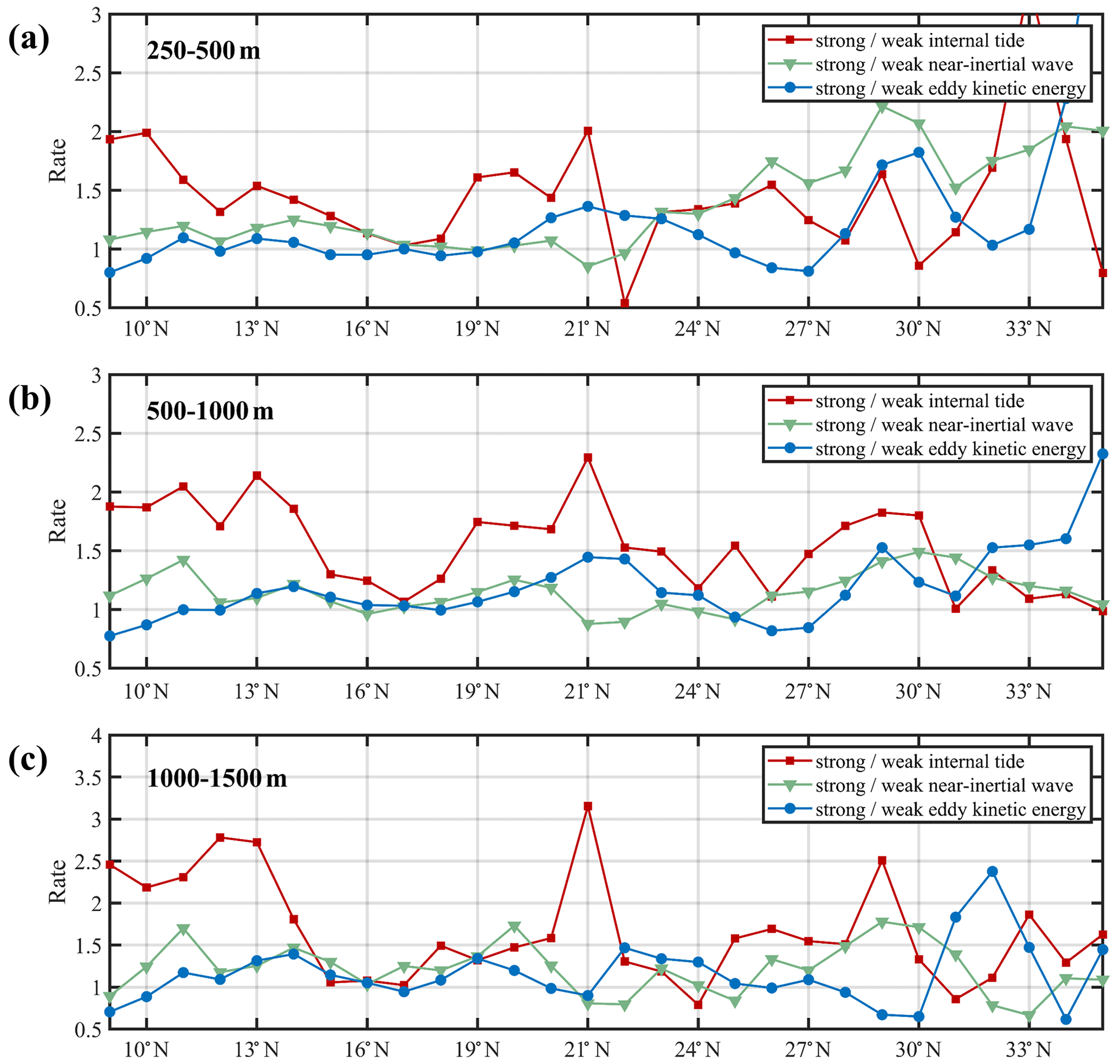
Figure 4 Ratios of diapycnal diffusivities between areas over strong (greater than median) and weak internal tides (red lines), strong (greater than median) and weak near-inertial waves (green lines), and strong (greater than median) and weak EKE (blue lines) for each 1^∘ latitude band in the depth ranges of (a) 250–500 m, (b) 500–1000 m, and (c) 1000–1500 m, which show averages for each band containing more than 10 estimates.

At depths of 250–500 m, the ratio associated with internal tides increased significantly at 10, 21, and 33^∘ N. These latitudes correspond to the Yap Trench, Luzon Strait, and Izu Ridge, which are mainly internal tidal source sites. The ratio reached 2 near these three latitudes, indicating that strong internal tides triggered the enhancement of K_z twice as much compared to the regions of weak internal tides. In addition, north of 23^∘ N, the ratio in relation to NIW in the upper ocean increased significantly with latitude, which indicated that the wind plays a more important role in mixing at this latitude band. This result is basically consistent with previous studies (Whalen et al., 2018), which suggested that the mixing is dominated by wind in the midlatitude. Taking the wind as the driving factor better explains the seasonal cycle of diapycnal diffusivities in Fig. 3, since the winds have an apparent seasonal dependence. The obvious seasonal trend of K_z due to the important contribution of wind occurs between 25–35^∘ N. In contrast, the ratio for wind is ∼1 at lower latitudes, indicating that the wind-driven mixing is insignificant here with the absence of wind-driven seasonal cycle.

The wind contribution to turbulent mixing is significantly reduced in the depth ranges of 500–1000 and 1000–1500 m (Fig. 4b and c). The ratio only increased slightly at midlatitudes and was less than 2 anywhere. In contrast, the enhancement of mixing triggered by internal tides at these depth ranges was more significant, with the ratios exceeding 3.5 at some latitudes. This suggested that internal tides played a more important role in deep ocean mixing. Furthermore, internal tides significantly enhanced K_z around 13, 21, and 29^∘ N, corresponding to the sources of the Mariana Trench, Luzon Strait, and Bonin Ridge, respectively. Such enhancement was not obvious at the Izu Ridge, possibly due to the shallower depth and paucity of deep data or the turning latitude effects in this area.

Combined with the analysis of relative contributions of different factors in different layers, it was concluded that the contribution of internal tides in turbulent mixing is more important in low latitudes of the Philippine Sea. In this area, the wind and mesoscale features did not significantly enhance K_z. At midlatitudes, internal tides still played an important role, but the wind contribution was more significant in the upper ocean. The wind drove turbulent mixing even at the depths of 500–1000 and 1000–1500 m. The midlatitude region not only corresponds to westerlies but also features energetic mesoscale motions. Therefore, the mesoscale features might be a potential factor for enhanced turbulent mixing. The modulation of the mesoscale environment in the wind-induced mixing has been discussed by some previous studies (e.g., Jing et al., 2011; Whalen et al., 2018), while the impact of mesoscale features in tide-induced mixing and in lower latitudes has not been considered.

The Philippine Sea was separated into two latitude bands. The vertical structures of diapycnal diffusivities in the regions with strong or weak internal tides were compared (Fig. 5). This result can directly reveal the enhancement of internal tide on mixing at different depths. A similar analysis was used for wind and EKE. In the low latitudes, K_z did not increase in the regions of high EKE or strong near-inertial energy, whereas it increased significantly in the regions of strong internal tides. This enhancement was more obvious below 400 m (Fig. 5a). And, in the midlatitudes, K_z in the upper ocean increased significantly, corresponding more to strong winds compared to weak winds (Fig. 5b). Meanwhile, K_z was also larger in the regions of strong internal tides and high EKE in the upper ocean. The enhancement of wind or EKE in turbulent mixing significantly weakened below 600 m, while the enhancement of internal tides increased with depth. Here, these results convey the following: (1) wind and EKE play important roles in mixing in the upper ocean and in the midlatitudes, and (2) strong internal tides facilitate and enhance mixing in the deeper ocean. These two conclusions are consistent with previous researchers (e.g., Jing et al., 2011; Whalen et al., 2012; Waterhouse et al., 2014; MacKinnon et al., 2017; Whalen et al., 2018). In addition, our results indicate that, in the Philippine Sea, internal tides play a significant role in turbulent mixing, not only in the low latitudes but also in the midlatitudes and not only in the deeper ocean but also in the upper ocean.

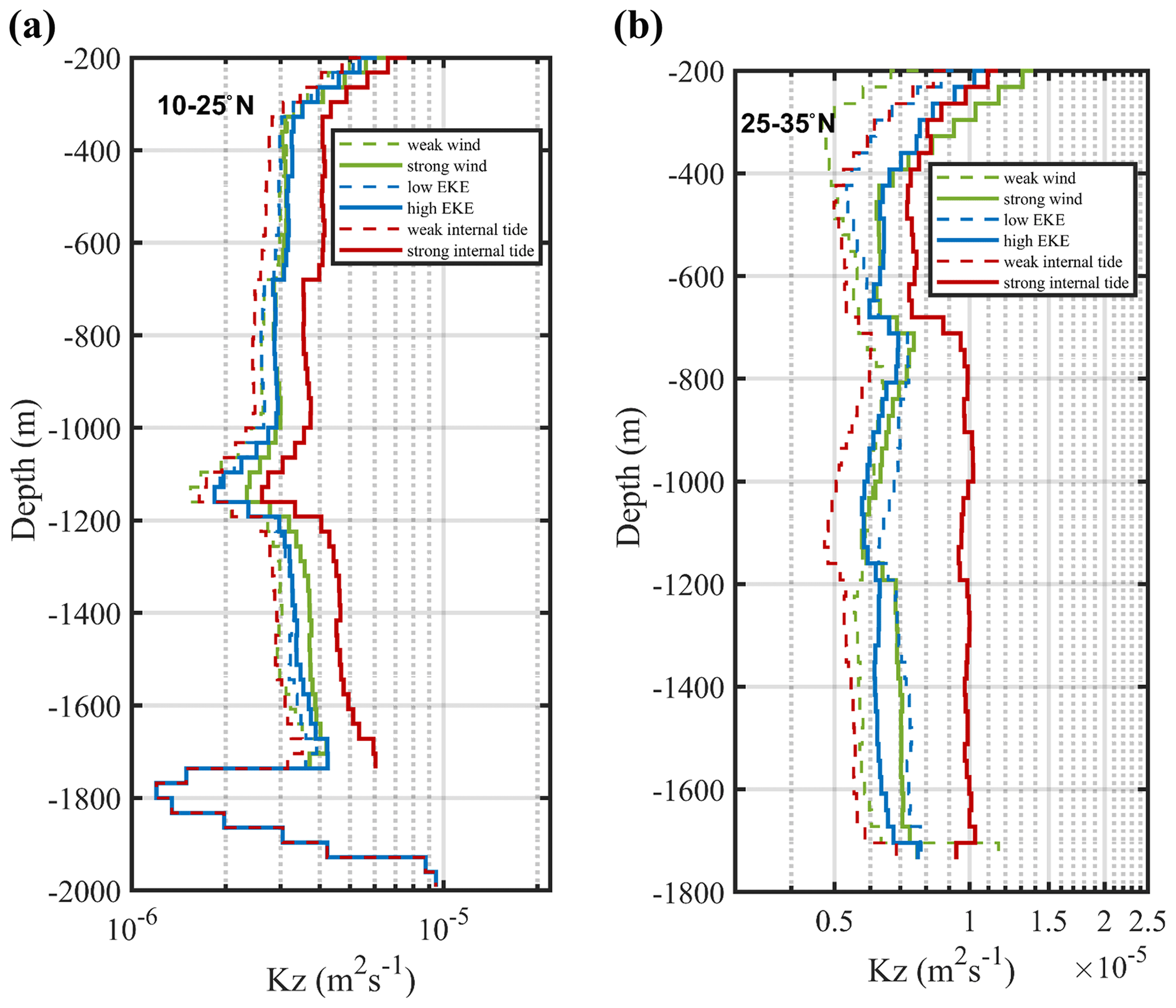
Figure 5 Vertical structures of geometric averaged diapycnal diffusivities K_z with weak and strong wind (green), low and high EKE (blue), and weak and strong internal tides (red) in the (a) low latitude and (b) midlatitude.

3.3.2 Wind

We adopted the linear regression approach and obtained the correlation between diapycnal diffusivities and wind. This approach generally uses statistics to derive the correlation between two factors (e.g., Wu et al., 2011; Jing and Wu, 2014; Jeon et al., 2018; Zhao, 2019). The regression coefficient is able to represent the mixing response to wind (e.g., Qiu et al., 2012). Here, the Philippine Sea is divided into 10–25 and 25–35^∘ N (Fig. 6). At a depth of 250–500 m, the slope is significantly larger in 25–35^∘ N (∼0.305) and smaller in 10–25^∘ N (∼0.029). The wind-driven turbulent mixing was most significant between 25–35^∘ N but was insignificant between 10–25^∘ N. At a depth of 500–1000 m, the wind influence on turbulent mixing was weakened in the midlatitudes. This was consistent with the results in Figs. 3 and 4. It proved that the contribution of wind has a latitudinal dependence, which was significant at the midlatitudes but insignificant at low latitudes. In addition, the response of turbulent mixing to wind weakened quickly with depth, indicating that the dominant factor of mixing in the deeper water column was not wind. Accordingly, it was difficult for wind to drive mixing below 1000 m, so we do not show the results at a depth of 1000–1500 m (Fig. 4).

Figure 6 Scatterplot of log-scale K_z versus log-scale, near-inertial energy flux from wind at 250–500 m between (a) 10–25^∘ N and (b) 25–35^∘ N and in 500–1000 m between (c) 10–25^∘ N and (d) 25–35^∘ N. The best fit slopes are denoted by the solid line, and the 95 % confidence interval is indicated by dashed lines.

3.3.3 Tide

The slopes of K_z to internal tide conversion rates represent the mixing response to internal tides. As discussed above, the mixing significantly responded to the internal tides over the entire Philippine Sea (Fig. 7). The relationship was depth dependent. The slopes did not reach 0.1 at a depth of 250–500 m, but increased significantly at 500–1000 and 1000–1500 m, and reached 0.128 for the deepest depth band. The response of mixing to internal tides was more significant in the deeper ocean. Focusing on different latitude bands, the slopes of K_z to internal tides is smaller at midlatitudes. This is because the wind contribution increased in this region, which led to a weakening relative contribution of internal tides. Compared with the internal tide conversion rates, the pattern of K_z was inconsistent with internal tides, even at lower latitudes. It can be inferred that the turbulent mixing was not only affected by the internal tides but also by other factors. There is a strong western boundary flow, i.e., the Kuroshio extension, and an active mesoscale environment in this region. Some researchers have shown that the existence of the mesoscale environment will alter the internal tide features, so we reasonably infer that the tide-induced turbulent mixing in this area was modulated by the mesoscale features.

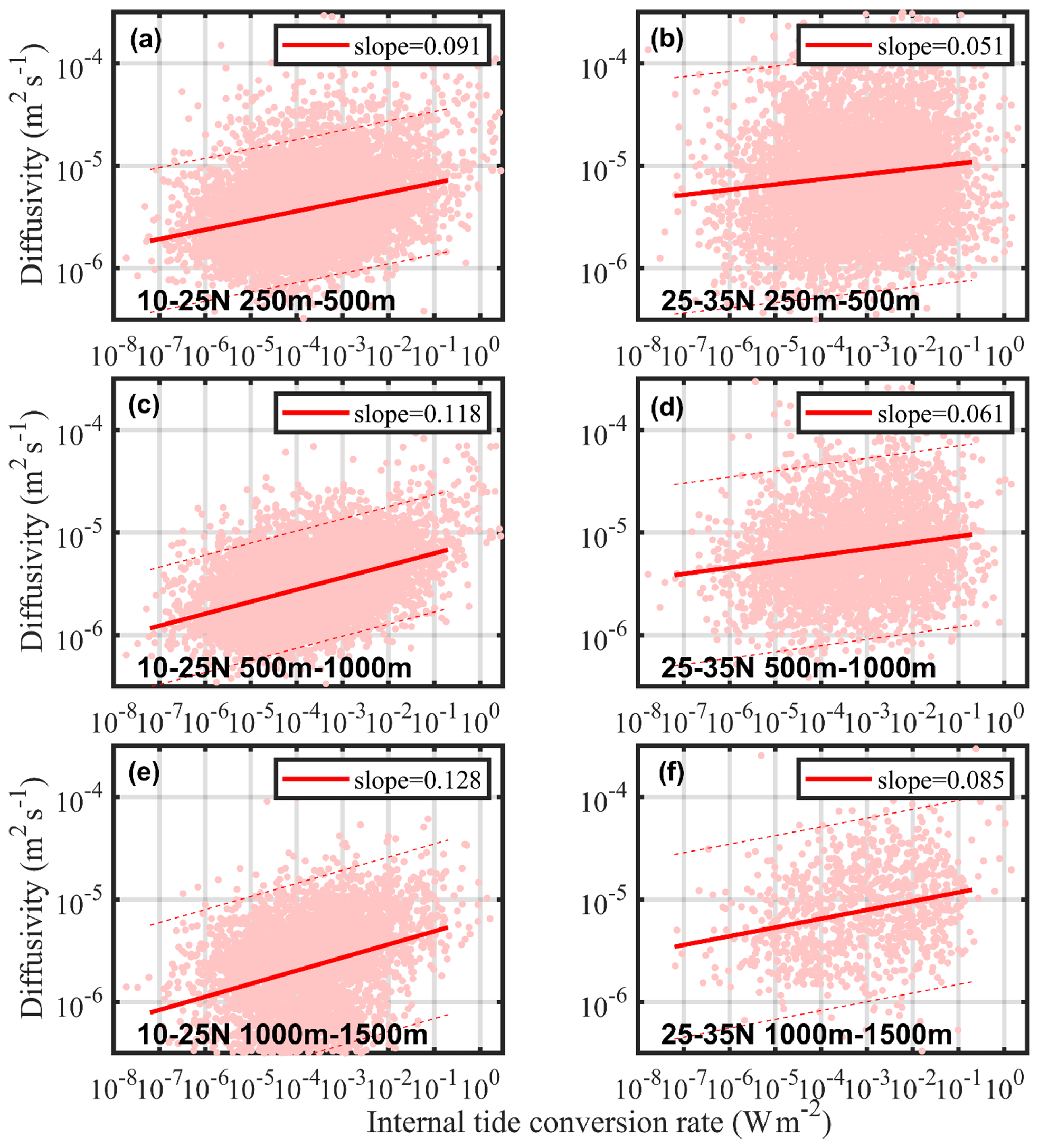
Figure 7 Scatterplot of log-scale K_z versus log-scale internal tide conversion rate at 250–500 m (a, b), 500–1000 m (c, d), and 1000–15 000 m (e, f), and the best fit slopes are denoted by the red line. Panels (a, c, e) and (b, d, f) are 10–25^∘ N and 25–35^∘ N latitude bands, respectively, and the 95 % confidence interval is indicated by dashed lines.

3.4 Role of mesoscale features in tidal mixing

Focusing on the low latitudes where tidal mixing dominated, the diapycnal diffusivities, K_z related to internal tides, and EKE are shown (Fig. 8). The combined influences of mesoscale features and internal tides on mixing are indicated. The increasing internal tide conversion rates significantly enhanced turbulent mixing. We find a correlation between elevated EKE and the averaged diapycnal diffusivities for a given internal tide conversion rate level. When the conversion rate was 10⁻³ W m⁻², the magnitudes of K_z were about 3 × 10⁻⁶ m² s⁻¹, 3 × 10⁻⁶ m² s⁻¹, and 1 × 10⁻⁶ m² s⁻¹ at depths of 250–500, 500–1000, and 1000–1500 m, respectively. When the internal tide conversion rates reached O(−1)–O(0), K_z reached 10⁻⁵ m² s⁻¹ at both depths of 250–500 and 500–1000 m and even exceeded 10⁻⁴ m² s⁻¹ at some internal tide source sites. In addition, there was a positive correlation between EKE and diapycnal diffusivity. A higher EKE can further increase K_z under the same magnitude of the internal tide conversion rate. Such an enhancement was more significant with strong internal tide conversion rates greater than 10⁻³ W m${}^{-\mathrm{2}}.$

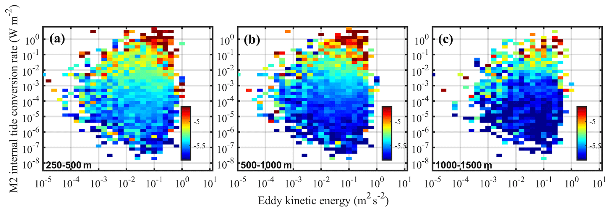
Figure 8 Averaged diapycnal diffusivities as a function of EKE and internal tide conversion rates between (a) 250–500 m, (b) 500–1000 m, and (c) 1000–1500 m.

M₂ and K₁ tidal constituents were analyzed to clarify the response of K_z to internal tides in the regions of high EKE (where the EKE is larger than the regional average value) and low EKE (Fig. 9). The results integrated eight main tidal constituents (Fig. 9a, b, and c) and showed that the slopes in a weak (strong) mesoscale field were smaller (larger), i.e., 0.081 (0.105), 0.103 (0.134), and 0.103 (0.142), at depths of 250–500, 500–1000, and 1000–1500 m, respectively. The turbulent mixing was more sensitive to the internal tide magnitude in the presence of an energetic mesoscale field. Moreover, such a response was more obvious in the region with strong internal tides (such as the >10⁻² W m⁻² conversion rate). In some regions with weak internal tides, such as those with internal tide conversion rates less than 10⁻³ W m⁻², the modulation of mesoscale eddies was less significant.

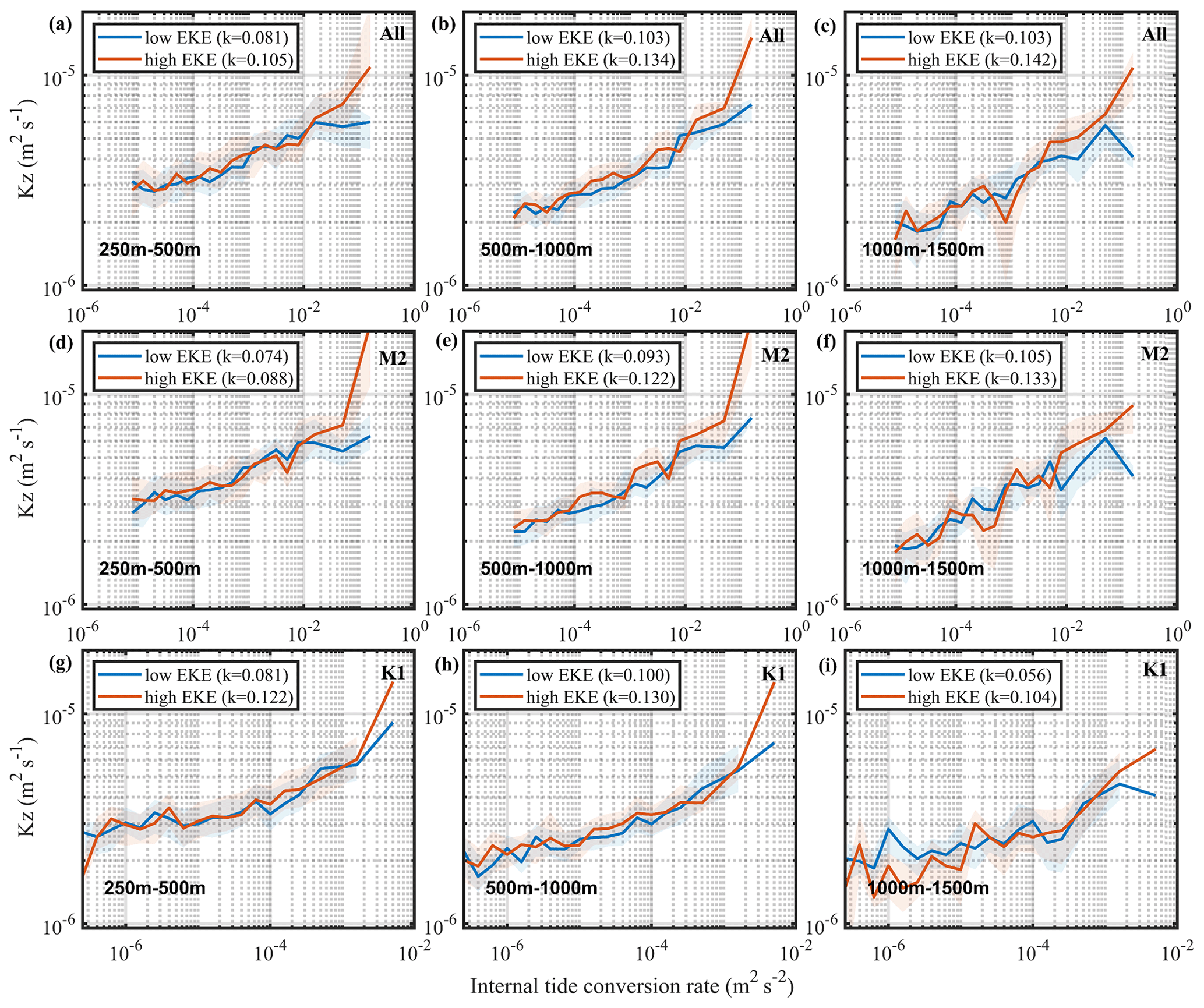
Figure 9 The averaged diffusivity between depths of (a, d, g) 250–500 m, (b, e, h) 500–1000 m, and (c, f, i) 1000–1500 m in high (greater than the median) and low (less than the median) EKE. The shading indicates 1 standard deviation. Panels (a, b, c), (d, e, f), and (g, h, i) are related to the eight main tidal constituents, M₂ internal tide, and K₁ internal tide, respectively.

A similar conclusion can be drawn when only considering M₂ or K₁. In regions of high EKE, the change in diffusivities in response to internal tides was significant, and the increase was more sensitive to the M₂ internal tide. The enhancement related to the M₂ internal tide was more significant below 500 m (Fig. 9d and e), while the enhancement of the K₁ internal tide was similar at all depths. This may be due to different features and structures of M₂ and K₁ internal tides. In this area, the modal structure and propagation path of the M₂ internal tide are more complicated and more prone to breaking, but those of K₁ were relatively stable, and this area includes the K₁ critical latitude range, which can be broadened by mesoscale currents (Robertson and Dong, 2019).

The modulation of cyclonic and anticyclonic eddies on tidal mixing also differs. The increase in K_z by internal tides in regions with cyclonic eddies (vorticity $\mathit{>}\mathrm{3}\times {\mathrm{10}}^{-\mathrm{6}}$ s⁻¹) and anticyclonic eddies (vorticity $\mathit{<}-\mathrm{3}\times {\mathrm{10}}^{-\mathrm{6}}$ s⁻¹) are both shown (Figs. 10 and 11). Under the same magnitude of internal tides, the K_z increases more significantly in the presence of anticyclonic eddies, which is obvious at 250–500 m, and can also be seen at 500–1000 m. Below 1000 m, there are no significant differences between the regions with cyclones and anticyclones.

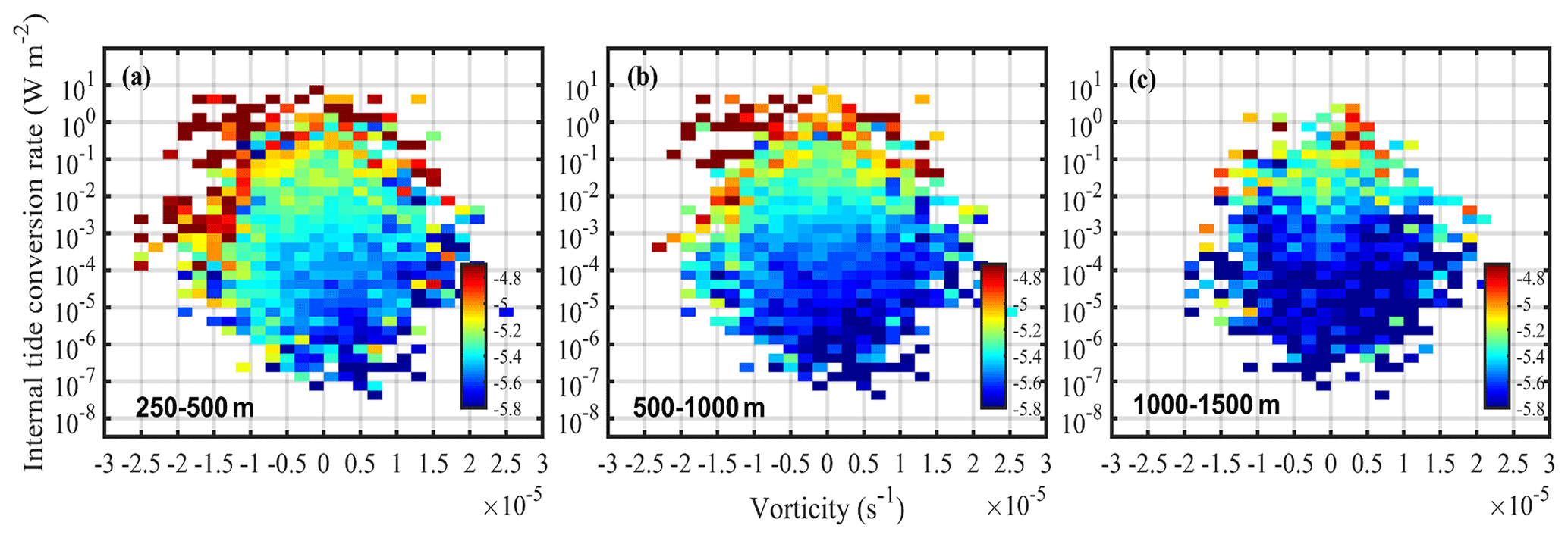
Figure 10 The averaged diapycnal diffusivities as a function of vorticity and internal tides conversion rate between (a) 250–500 m, (b) 500–1000 m, and (c) 1000–1500 m.

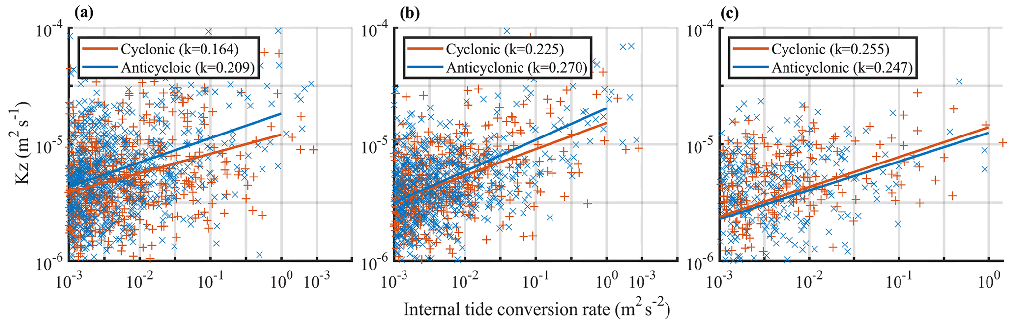
Figure 11 Scatterplot of log-scale K_z versus log-scale internal tide conversion rate, with cyclone (red) and anticyclone (blue), at (a) 250–500 m, (b) 500–1000 m, and (c) 1000–1500 m. The best fit slopes are denoted by the red and blue solid lines.

Considering that mixing driven by eddies is relatively significant in regions where the tidal mixing is very weak, we only analyze the cases of internal tide conversion rates larger than 10⁻³ W m${}^{-\mathrm{2}}.$ When the conversion rates become larger than this value, the diapycnal diffusivities in the presence of high EKE increase faster with internal tides (Fig. 9). It was found that the response of turbulent mixing to internal tides was more sensitive in the presence of anticyclones above 1000 m, while, below 1000 m, the influence of cyclones is slightly stronger than that of anticyclones.

4 Summary

The spatial pattern and seasonal variability in the diapycnal diffusivities in the Philippine Sea were estimated using a fine-scale parameterization. The main conclusions follow.

The seasonal fluctuations in mixing in this area were zonally dependent. Seasonal variability was strong in winter and weak in summer at midlatitudes, with the seasonal fluctuations being more obvious in the upper ocean. This was attributed to the westerlies, and the wind plays a more significant role in turbulent mixing here. However, the seasonal cycle of mixing in the low latitudes was not obvious, indicating that the wind-driven mixing was not dominant here. As opposed to wind-driven mixing, tidal mixing was more significant in the deeper ocean.

Evidence that the mixing was modulated by internal tides was seen in regions of both high and low EKE, and it was more significant with high EKE. The presence of high EKE enhanced the response of K_z to internal tides, especially for the M₂ internal tide. The increased rate of K_z with internal tides in the high EKE field was higher than that in the weak EKE field. The existence of mesoscale features changed the vertical structure of internal tides and transferred the internal tides energy from low modes to higher modes. It was more likely to cause internal tide breaking (Dunphy and Lamb, 2014). The enhancement by mesoscale motions in tidal mixing was more significant for M₂ internal tides. Anticyclonic eddies were more likely to increase tidal mixing in the upper ocean, while the influence of cyclonic eddies to tidal mixing was slightly higher than that of anticyclonic ones in the deep ocean.

There are several mechanisms that might explain the elevated tidal mixing in the present of energetic mesoscale environment. The vertical scales of internal tides can be reduced and the energy of internal tides can be amplified near the surface in the presence of energetic mesoscale features. When the internal tide passes through a mesoscale eddy, the energy of the mode 1 internal tide can be refracted and transmitted to higher-mode waves (e.g., Farrari and Wunsch, 2008; Henning and Vallis, 2005). The eddy flows can also directly increase vertical shear and, subsequently, the internal tide energy dissipation rate (e.g., Chavanne et al., 2010; Dunphy and Lamb, 2014). The anticyclones induce higher tidal mixing than cyclones, probably because of the chimney effects associated with distinct vorticities (Jing et al., 2011).

This paper explores the modulation of the mesoscale environments on tide-induced mixing statistically through Argo float observations. Theoretical clarification of the driving mechanisms is needed. Some previous numerical studies can explain our conclusion to some extent. However, how and to which extent the vorticity alters internal tide evolution and induced mixing has not been clearly explained in theory. Moreover, the latitude ranges, from 9 to 36^∘ N discussed in this work, are due to the limitations of the fine-scale parameterization method in equatorial areas. The influence of the equatorial background flows on ocean mixing remains to be solved.