the Creative Commons Attribution 4.0 License.
the Creative Commons Attribution 4.0 License.
 | 19 May 2021
Magnetospheric chaos and dynamical complexity response during storm time disturbance
Irewola Aaron Oludehinwa
Olasunkanmi Isaac Olusola
Olawale Segun Bolaji
Olumide Olayinka Odeyemi
Abdullahi Ndzi Njah
In this study, we examine the magnetospheric chaos and dynamical complexity response to the disturbance storm time (Dst) and solar wind electric field (VBs) during different categories of geomagnetic storm (minor, moderate and major geomagnetic storm). The time series data of the Dst and VBs are analysed for a period of 9 years using non-linear dynamics tools (maximal Lyapunov exponent, MLE; approximate entropy, ApEn; and delay vector variance, DVV). We found a significant trend between each non-linear parameter and the categories of geomagnetic storm. The MLE and ApEn values of the Dst indicate that chaotic and dynamical complexity responses are high during minor geomagnetic storms, reduce at moderate geomagnetic storms and decline further during major geomagnetic storms. However, the MLE and ApEn values obtained from VBs indicate that chaotic and dynamical complexity responses are high with no significant difference between the periods that are associated with minor, moderate and major geomagnetic storms. The test for non-linearity in the Dst time series during major geomagnetic storm reveals the strongest non-linearity features. Based on these findings, the dynamical features obtained in the VBs as input and Dst as output of the magnetospheric system suggest that the magnetospheric dynamics are non-linear, and the solar wind dynamics are consistently stochastic in nature.
- Article
(476 KB) - Full-text XML
- BibTeX
- EndNote


The response of chaos and dynamical complexity behaviour with respect to magnetospheric dynamics varies (Tsurutani et al., 1990). This is due to changes in the interplanetary electric fields imposed on the magnetopause and those penetrating the inner magnetosphere and sustaining convection, thereby initiating a geomagnetic storm (Dungey, 1961; Pavlos et al., 1992). A prolonged southward turning of interplanetary magnetic field (IMF, Bz), which indicates that solar-wind–magnetosphere coupling is in progress, was confirmed on many occasions for which such a geomagnetic storm was driven by co-rotating interaction regions (CIRs), by the sheath preceding an interplanetary coronal mass ejection (ICME), or by a combination of the sheath and an ICME magnetic cloud (Gonzalez and Tsurutani, 1987; Tsurutani and Gonzalez, 1987; Tsurutani et al., 1988; Cowley, 1995; Tsutomu, 2002; Yurchyshyn et al., 2004; Kozyra et al., 2006; Echer et al., 2008; Meng et al., 2019; Tsurutani et al., 2020; Echer et al., 2006). The sporadic magnetic reconnection between the southward component of the Alfvén waves and the earth's magnetopause leads to isolated substorms or convection events such as the high-intensity long-duration continuous AE activity (HILDCAA, where AE represents auroral electrojet) which are shown to last from days to weeks (Akasofu, 1964; Tsurutani and Meng, 1972; Meng et al., 1973; Tsurutani and Gonzalez, 1987; Hajra et al., 2013; Liou et al., 2013; Mendes et al., 2017; Hajra and Tsurutani, 2018; Tsurutani and Hajra, 2021; Russell, 2001). Notably, the introduction of the disturbance storm time (Dst) index (Sugiura, 1964; Sugiura and Kamei, 1991) unveiled a quantitative measure of the total energy of the ring current particles. Therefore, the Dst index remains one of the most popular global indicators that can precisely reveal the severity of a geomagnetic storm (Dessler and Parker, 1959).
The Dst fluctuations exhibit different signatures for different categories of geomagnetic storm. Ordinarily, one can easily anticipate that fluctuations in a Dst signal appear chaotic and complex. These may arise from the changes in the interplanetary electric fields driven by the solar-wind–magnetospheric coupling processes. At different categories of geomagnetic storm, fluctuations in the Dst signals differ (Oludehinwa et al., 2018). One obvious reason is that as the intensity of the geomagnetic storm increases, the fluctuation behaviour in the Dst signal becomes more complex and non-linear in nature. It has been established that the electrodynamic response of the magnetosphere to solar wind drivers are non-autonomous in nature (Price and Prichard, 1993; Price et al., 1994; Johnson and Wings, 2005). Therefore, the chaotic analysis of the magnetospheric time series must be related to the concept of input–output dynamical process (Russell et al., 1974; Burton et al., 1975; Gonzalez et al., 1989, 1994). Consequently, it is necessary to examine the chaotic behaviour of the solar wind electric field (VBs) as input signals and the magnetospheric activity index (Dst) as output during different categories of geomagnetic storms.
Several works have been presented on the chaotic and dynamical complexity behaviour of the magnetospheric dynamics based on an autonomous concept, i.e. using the time series data of magnetospheric activity alone such as auroral electrojet (AE), amplitude lower (AL) and Dst index (Vassiliadis et al., 1990; Baker and Klimas, 1990; Vassiliadis et al., 1991; Shan et al., 1991; Pavlos, 1994; Klimas et al., 1996; Valdivia et al., 2005; Mendes et al., 2017; Consolini, 2018). Authors found evidence of low-dimensional chaos in the magnetospheric dynamics. For instance, the report by Vassiliadis et al. (1991) shows that the computation of Lyapunov exponent for AL index time series gives a positive value of Lyapunov exponent, indicating the presence of chaos in the magnetospheric dynamics. Unnikrishnan (2008) studied the deterministic chaotic behaviour in the magnetospheric dynamics under various physical conditions using AE index time series and found that the seasonal mean value of Lyapunov exponent in winter season during quiet periods (0.7±0.11 min−1) is higher than that of the stormy periods (0.36±0.09 min−1). Balasis et al. (2006) examined the magnetospheric dynamics in the Dst index time series from pre-magnetic storm to magnetic storm period using fractal dynamics. They found that the transition from anti-persistent to persistent behaviour indicates that the occurrence of an intense geomagnetic storm is imminent. Balasis et al. (2009) further reveal the dynamical complexity behaviour in the magnetospheric dynamics using various entropy measures. They reported a significant decrease in dynamical complexity and an accession of persistency in the Dst time series as the magnetic storm approaches. Recently, Oludehinwa et al. (2018) examined the non-linearity effects in Dst signals during minor, moderate and major geomagnetic storms using recurrence plots and recurrence quantification analyses. They found that the dynamics of the Dst signal is stochastic during minor geomagnetic storm periods and deterministic as the geomagnetic storm increases.
Also, studies describing the solar wind and magnetosphere as a non-autonomous system have been extensively investigated. Price et al. (1994) examine the non-linear input–output analysis of AL index and different combinations of interplanetary magnetic field (IMF) with solar wind parameters as input functions. They found that only a few of the input combinations show any evidence whatsoever for non-linear coupling between the input and output for the interval investigated. Pavlos et al. (1999) presented further evidence of magnetospheric chaos. They compared the observational behaviour of the magnetospheric system with the results obtained by analysing different types of stochastic and deterministic input–output systems and asserted that a low-dimensional chaos is evident in magnetospheric dynamics. Prabin Devi et al. (2013) studied the magnetospheric dynamics using AL index and the southward component of IMF (Bz). They observed that the magnetosphere and turbulent solar wind have values corresponding to non-linear dynamical system with chaotic behaviour. The modelling and forecasting approach have been applied to magnetospheric time series using non-linear models (Valdivia et al., 1996; Vassiliadis et al., 1999; Vassiliadis, 2006; Balikhin et al., 2010). These efforts have improved our understanding that the concept of non-linear dynamics can reveal some hidden dynamical information in the observational time series. In addition to these non-linear effects in Dst signals, a measure of the exponential divergence and convergence within the trajectories of a phase space known as maximal Lyapunov exponent (MLE), which has the potential to depict the chaotic behaviour in the Dst and VBs time series during a minor, moderate or major geomagnetic storm, has not been investigated. In addition, to the best of our knowledge, computation of approximate entropy (ApEn) that depicts the dynamical complexity behaviour during different categories of geomagnetic storm has not been reported in the literature. The test for non-linearity through delay vector variance (DVV) analysis that reveals the non-linearity features in Dst and VBs time series during minor, moderate and major geomagnetic storms is not well known. It is worthy to note that understanding the dynamical characteristics in the Dst and VBs signals at different categories of geomagnetic storms will provide useful diagnostic information to different conditions of space weather phenomenon. Consequently, this study attempts to carry out comprehensive numerical analyses to unfold the chaotic and dynamical complexity behaviour in the Dst and VBs signals during minor, moderate and major geomagnetic storms. In Sect. 2, our methods of data acquisition are described. Also, the non-linear analysis that we employed in this investigation is detailed. In Sect. 3, we unveil our results and engage in the discussion of results in Sect. 4.
The Dst index is derived by measurements from ground-based magnetic stations at low-latitude observatories around the world and depicts mainly the variation of the ring current, as well as the Chapman–Ferraro magnetopause currents, and tail currents to a lesser extent (Sugiura, 1964; Feldstein et al., 2005, 2006; Love and Gannon, 2009). Due to its global nature, the Dst time series provides a measure of how intense a geomagnetic storm was (Dessler and Parker, 1959). In this study, we considered Dst data for the period of 9 years from January to December between 2008 and 2016 which were downloaded from the World Data Centre for Geomagnetism, Kyoto, Japan (http://wdc.kugi.kyoto-u.ac.jp/dst_final/index.html, last access: 15 May 2021). We use the classification of geomagnetic storms as proposed by Gonzalez et al. (1994) such that Dst index value in the ranges nT, nT and nT are classified as minor, moderate and major geomagnetic storms, respectively, and each time series is being classified based on its minimum Dst value. The solar wind electric field (VBs) data are archived from the National Aeronautics and Space Administration, Space Physics Facility (https://omniweb.gsfc.nasa.gov/form/dx1.html, last access: 15 May 2021). The sampling time of Dst and VBs time series data was 1 h. It is well known that the dynamics of the solar wind contribute to the driving of the magnetosphere (Burton et al., 1975). Furthermore, we took the solar wind electric field (VBs) as the input signal (Price and Prichard, 1993; Price et al., 1994). The VBs was categorized according to the periods of minor, moderate and major geomagnetic storms. Then, the Dst and VBs time series were subjected to a variety of non-linear analytical tools explained as follows.
2.1 Phase space reconstruction and observational time series
An observational time series can be defined as a sequence of scalar measurements of some quantity, which is a function of the current state of the system taken at multiples of a fixed sampling time. In non-linear dynamics, the first step in analysing an observational time series is to reconstruct an appropriate state space of the system. Takens (1981) and Mañé (1981) stated that one time series or a few simultaneous time series are converted to a sequence of vectors. This reconstructed phase space has all the dynamical characteristic of the real phase space provided the time delay and embedding dimension are properly specified.
where X(t) is the reconstructed phase space, x(t) is the original time series data, τ is the time delay and m is the embedding dimension. An appropriate choice of τ and m is needed for the reconstruction of phase space, which is determined by average mutual information and false nearest neighbour, respectively.
2.2 Average mutual information (AMI)
The method of average mutual information (AMI) is one of the non-linear techniques used to determine the optimal time delay (τ) required for phase space reconstruction in observational time series. The time delay mutual information was proposed by Fraser and Swinney (1986) instead of an autocorrelation function. This method takes into account non-linear correlations within the time series data. It measures how much information can be predicted about one time series point, given full information about the other. For instance, the mutual information between xi and x(i+τ) quantifies the information in state x(i+τ) under the assumption that information at the state xi is known. The AMI for a time series x(ti), is calculated as
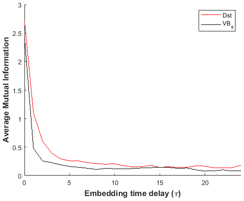
where x(ti) is the ith element of the time series, T=kΔt (), P(x(ti)) is the probability density at x(ti), and is the joint probability density at the pair xt(ti) and x(ti+T). The time delay (τ) of the first minimum of AMI is chosen as optimal time delay (Fraser and Swinney, 1986; Fraser, 1986). Therefore, the AMI was applied to the Dst and VBs time series, and the plot of AMI versus time delay is shown in Fig. 3. We notice that the AMI showed the first local minimum at roughly τ=15 h. Furthermore, the values of τ near this value of ∼ 15 h maintain constancy for both VBs and Dst. In the analysis, τ=15 h was used as the optimal time delay for the computation of maximal Lyapunov exponent.
2.3 False nearest neighbour (FNN)
In determining the optimal choice of embedding dimension (m), the false nearest neighbour method was used in the study. The method was suggested by Kennel et al. (1992). The concept is based on how the number of neighbours of a point along a signal trajectory changes with increasing embedding dimension. With increasing embedding dimension, the false neighbour will no longer be neighbours; therefore, by examining how the number of neighbours changes as a function of dimension, an appropriate embedding dimension can be determined. For instance, suppose we have a one-dimensional time series. We can construct a time series y(t) of D-dimensional points from the original one-dimensional time series x(t) as follows:
where τ and D are time delay and embedding dimension. Using the formula from Kennel et al. (1992) and Wallot and Monster (2018), if we have a D-dimensional phase space and denote the rth nearest neighbour of a coordinate vector y(t) by y(r)(t), then the square of the Euclidean distance between y(t) and the rth nearest neighbour is
Now applying the logic outlined above, we can go from a D-dimensional phase space to D+1-dimensional phase space by time-delay embedding, adding a new coordinate to y(t), and ask what is the squared distance between y(t) and the same rth nearest neighbour:
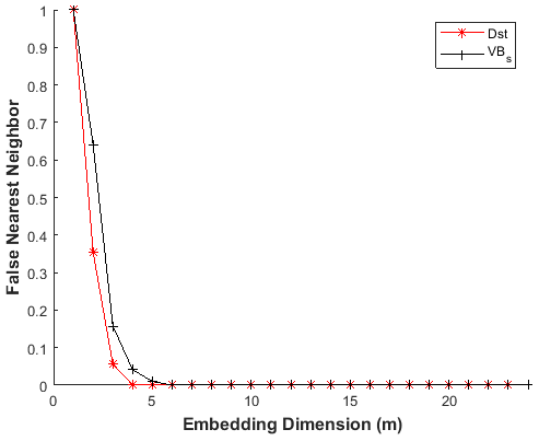
As explained above, if the one-dimensional time series is already properly embedded in D dimensions, then the distance R between y(t) and the rth nearest neighbour should not change appreciably by some distance criterion Rtol (i.e. R<Rtol). Moreover, the distance of the nearest neighbour when embedded into the next higher dimension relative to the size of the attractor should be less than some criterion Atol (i.e. ). Doing this for the nearest neighbour of each coordinate will result in many false nearest neighbours when embedding is insufficient or in few (or no) false neighbours when embedding is sufficient. In the analysis, the FNN was applied to the Dst and VBs time series to detect the optimal value of embedding dimension (m). Figure 4 shows a sample plot of the percentage of false nearest neighbour against embedding dimension in one of the months under investigation (other months show similar results; thus, for brevity we depict only one of the results). We notice that the false nearest neighbour attains its minimum value at m≥5, indicating that embedding dimension (m) values from m≥5 are optimal. Therefore, m=5 was used for the computation of maximal Lyapunov exponent.
2.4 Maximal Lyapunov exponent (MLE)
The maximal Lyapunov exponent (MLE) is one of the most popular non-linear dynamics tools used for detecting chaotic behaviour in a time series. It describes how small changes in the state of a system grow at an exponential rate and eventually dominate the behaviour. An important indication of chaotic neighbour of a dissipative deterministic system is the existence of a positive Lyapunov exponent. A positive MLE signifies divergence of trajectories in one direction or expansion of an initial volume in this direction. On the other hand, a negative MLE exponent implies convergence of trajectories or contraction of volume along another direction. The algorithm proposed by Wolf et al. (1985) for estimating MLE is employed to compute the chaotic neighbour of the Dst and VBs time series at minor, moderate and major geomagnetic storms. Other methods of determining MLE include Rosenstein's method, Kantz's method and so on. In this study, the MLE for minor, moderate and major geomagnetic storm periods was computed with m=5 and τ=15 h as shown in Figs. 5 and 6 (bar plots) for Dst and VBs. The calculation of MLE is explained as follows: given a sequence of vector x(t), an m-dimensional phase space is formed from the observational time series through an embedding theorem as
where m and τ are as defined earlier; after reconstructing the observational time series, the algorithm locates the nearest neighbour (in Euclidean sense) to the initial point and denotes the distance between these two points L(t0). At a later point t1, the initial length will have evolved to length L′(t1). Then the MLE is calculated as
where M is the total number of replacement steps. We look for a new data point that satisfies two criteria reasonably well: its separation, L(t1), from the evolved fiducial point is small. If an adequate replacement point cannot be found, we retain the points that were being used. This procedure is repeated until the fiducial trajectory has traversed the entire data.
2.5 Approximate entropy (ApEn)
Approximate entropy (ApEn) is one of the non-linear dynamics tools that measures the dynamical complexity in observational time series. The concept was proposed by Pincus (1991), who provide a generalized measure of regularity, such that it accounts for the logarithm likelihood in the observational time series. For instance, a dataset of length N that repeat itself for m points within a boundary will again repeat itself for m+1 points. Because of its computational advantage, ApEn has been widely used in many disciplines to study dynamical complexity (Pincus and Kalman, 2004; Pincus and Goldberger, 1994; McKinley et al., 2011; Kannathan et al., 2005; Balasis et al., 2009; Shujuan and Weidong, 2010; Moore and Marchant, 2017). The ApEn is computed using the formula below:
where is the correlation integral, m is the embedding dimension and r is the tolerance. To compute the ApEn for the Dst and VBs time series classified as minor, moderate and major geomagnetic storms from 2008 to 2016, we choose m=3 and τ=1 h. We refer interested readers to the works of Pincus (1991), Kannathal et al. (2005) and Balasis et al. (2009) where all the computational steps regarding ApEn were explained in detail. Figures. 5 and 6 depict the stem plot of ApEn for Dst and VBs from 2008 to 2016.
2.6 Delay vector variance (DVV) analysis
The delay vector variance (DVV) is a unified approach in analysing and testing for non-linearity in a time series (Gautama et al., 2004; Mandic et al., 2007). The basic idea of the DVV is that if two delay vectors of a predictable signal are close to each other in terms of the Euclidean distance, they should have a similar target. For instance, when a time delay (τ) is embedded into a time series x(k), , then a reconstructed phase space vector is formed which represents a set of delay vectors (DVs) of a given dimension.
Reconstructing the phase space, a set (λk) is generated by grouping those DVs that are within a certain Euclidean distance to DVs (X(k)). For a given embedding dimension (m), a measure of unpredictability σ∗2 is computed over all pairwise Euclidean distances between delay vector as
Then, sets λk(rd) are generated as the sets which consist of all delay vectors that lie closer to x(k) than a certain distance rd.
For every set λk(rd), the variance of the corresponding target σ∗2(rd) is
where σ∗2(rd) is target variance against the standardized distance, indicating that Euclidean distance will be varied in a manner standardized with respect to the distribution of pairwise distance between DVs. The iterative amplitude-adjusted Fourier transform (IAAFT) method is used to generate the surrogate time series (Kugiumtzis, 1999). If the surrogate time series yields a DV plots similar to the original time series and the scattered plot coincides with the bisector line, then the original time series can be regarded as linear (Theiler et al., 1992; Gautama et al., 2004; Imitaz, 2010; Jaksic et al., 2016). On the other hand, if the surrogate time series yields DV plot that is not similar to that of the original time series, then the deviation from the bisector lines indicates non-linearity. The deviation from the bisector lines grows as a result of the degree of non-linearity in the observational time series.
where ) is the target variance at the span rd for the ith surrogate. To carry out the test for non-linearity in the Dst signals (m=3, nd=3), the number of reference DVs = 200 and the number of surrogates Ns=25 were used in all of the analysis. Then we examined the non-linearity response at minor, moderate and major geomagnetic storms.
In this study, Dst and VBs time series from January to December were analysed for the period of 9 years (2008 to 2016) to examine the chaotic and dynamical complexity response in the magnetospheric dynamics during minor, moderate and major geomagnetic storms. Figures 1 and 2 display the samples of fluctuation signatures of Dst and VBs signals classified as (a) minor, (b) moderate and (c) major geomagnetic storms. The plot of average mutual information against time delay (τ) shown in Fig. 3 depicts that the first local minimum of the AMI function was found to be roughly at τ=15 h. Furthermore, we notice that the values of τ near this value of ∼ 15 h maintain constancy for both VBs and Dst. Also, in Fig. 4, we display the plot of the percentage of false nearest neighbour against embedding dimension (m). It is obvious that a decrease in false nearest neighbour when increasing the embedding dimension drops steeply to zero at the optimal dimension (m=5); thereafter, the false neighbours stabilize at that m=5 for VBs and Dst. Therefore, m=5 and τ=15 h were used for the computation of MLE at different categories of geomagnetic storm, while m=3 and τ=1 h are applied for the computation of ApEn values.

Figure 1Samples of Dst signals classified as (a) minor, (b) moderate and (c) major geomagnetic storms.
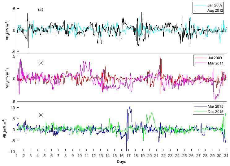
Figure 2Samples of solar wind electric fields (VBs) during (a) minor, (b) moderate and (c) major geomagnetic storms.
The results of MLE (bar plot) and ApEn (stem plot) for Dst at minor, moderate and major geomagnetic storms are shown in Fig. 5. During minor geomagnetic storms, we notice that the value of MLE ranges between 0.07 and 0.14 for most of the months classified as minor geomagnetic storms. Similarly, the ApEn (stem plot) ranges between 0.59 and 0.83. It is obvious that strong chaotic behaviour with high dynamical complexity are associated with minor geomagnetic storms. During moderate geomagnetic storms, (see Fig. 5b), we observe a reduction in MLE values (0.04–0.07) compared to minor geomagnetic storm periods. Within the observed values of MLE during moderate geomagnetic storms, we found a slight rise of MLE in the following months: March in 2008; April in 2011; January, February, and April in 2012; July, August, September, October, and November in 2015; and November in 2016. Also, the ApEn revealed a reduction in values between 0.44 and 0.57 during moderate geomagnetic storms. The lowest values of ApEn were noticed in the following months: May 2010, March 2011 and January 2016. During major geomagnetic storms as shown in Fig. 5, the minimum and maximum values of MLE are respectively 0.03 and 0.04, implying a very strong reduction of chaotic behaviour compared with minor and moderate geomagnetic storms. The lowest values of MLE were found in the months of July 2012, June 2013 and March 2015. Interestingly, further reduction in ApEn value (0.29–0.40) was as well noticed during this period. Thus, during major geomagnetic storms, chaotic behaviour and dynamical complexity subside significantly.
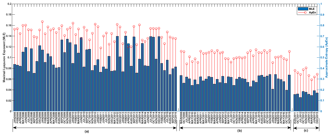
Figure 5The MLE (bar plot) and ApEn (stem plot) of Dst at (a) minor, (b) moderate and (c) major geomagnetic storms.
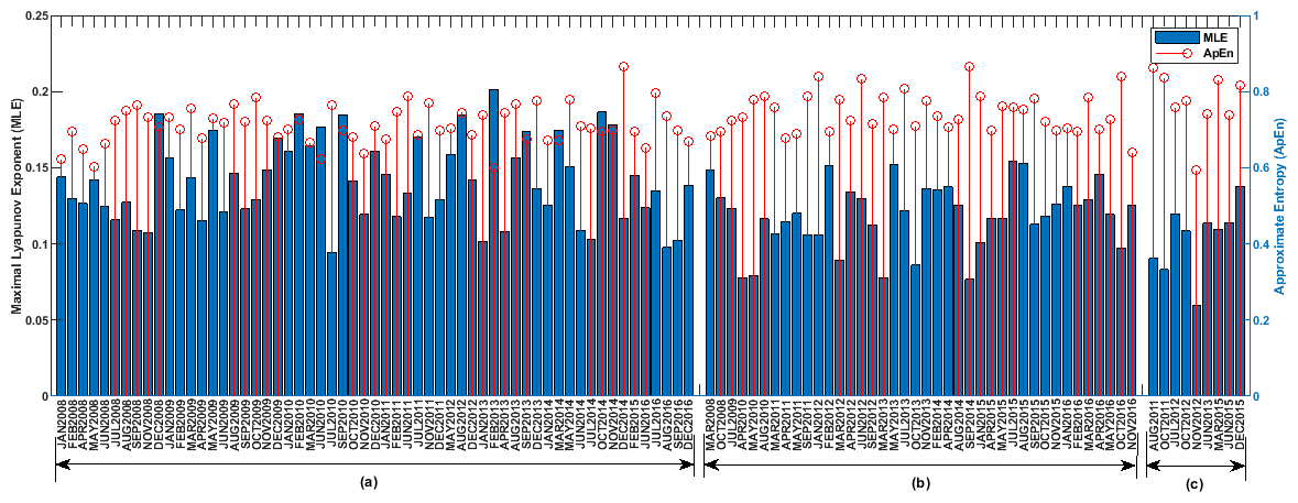
Figure 6The MLE (bar plot) and ApEn (stem plot) of solar wind electric field (VBs) during: (a) minor, (b) moderate and (c) major geomagnetic storms.
We display in Fig. 6 the results of MLE and ApEn computation for the VBs which has been categorized according to the periods of minor, moderate and major geomagnetic storms. The values of MLE (bar plot) were between 0.06 and 0.20 for VBs. The result obtained indicates strong chaotic behaviour with no significant difference in chaoticity during minor, moderate and major geomagnetic storms. Similarly, the results obtained from computation of ApEn (stem plot) for VBs depict a minimum value of 0.60 and peak value of 0.87 as shown in Fig. 6. The ApEn values of VBs indicates high dynamical complexity response with no significant difference during the periods of the three categories of geomagnetic storm investigated.
The test for non-linearity in the Dst signals during minor, moderate and major geomagnetic storms was analysed through the DVV analysis. Shown in Fig. 7 is the DVV plot and DVV scatter plot during minor geomagnetic storms for January 2009 and January 2014. We found that the DVV plots during minor geomagnetic storms reveals a slight separation between the original and surrogate data. Also, the DVV scatter plots show a slight deviation from the bisector line between the original and surrogate data which implies non-linearity. Also, during moderate geomagnetic storms, we notice that the DVV plot depicts a wide separation between the original and the surrogate data. Also, a large deviation from the bisector line between the original and the surrogate data was also noticed in the DVV scatter plot as shown in Fig. 8 thus indicating non-linearity. In Fig. 9, we display samples of DVV plot and DVV scatter plot during major geomagnetic storm for October 2011 and December 2015. The original and the surrogate data showed a very large separation in the DVV plot during major geomagnetic storm. The DVV scatter plot depicts the greatest deviation from the bisector line between the original and the surrogate data which is also an indication of non-linearity. The DVV analysis of the VBs time series during minor, moderate and major geomagnetic storms shown in Figs. 10–12 revealed a separation between the original and surrogate data with no significant difference between the periods of minor, moderate and major geomagnetic storms.
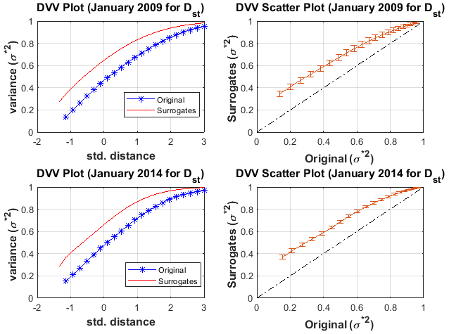
Figure 7The DVV plot and scatter plot for Dst during minor geomagnetic storm for January 2009 and January 2014.
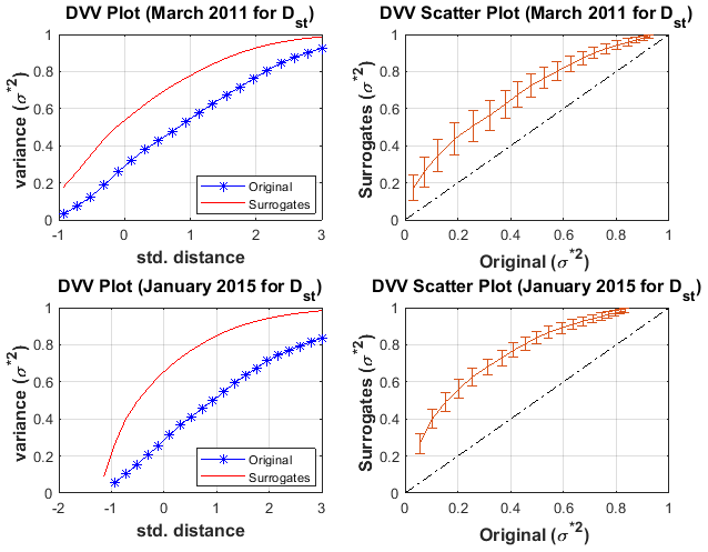
Figure 8The DVV plot and scatter plot for Dst during moderate geomagnetic storm for March 2011 and January 2015.
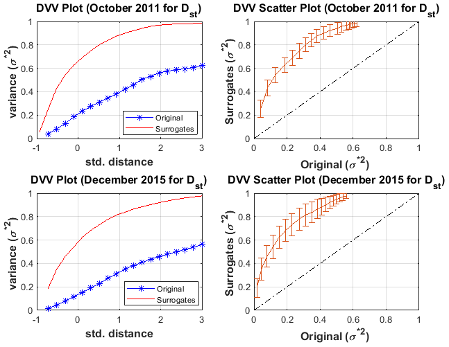
Figure 9The DVV plot and scatter plot for Dst during major geomagnetic storm for October 2011 and December 2015.
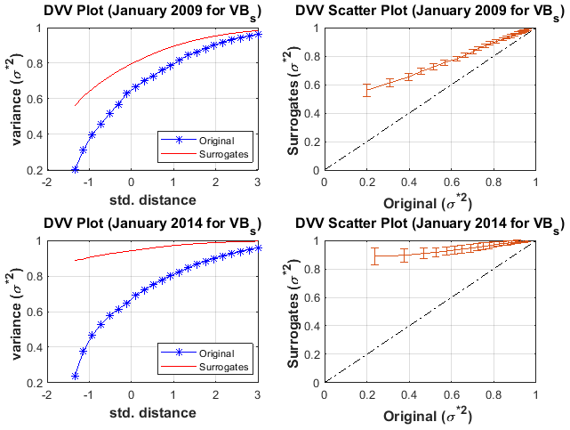
Figure 10The DVV plot and scatter plot for VBs during minor geomagnetic storm for January 2009 and January 2014.
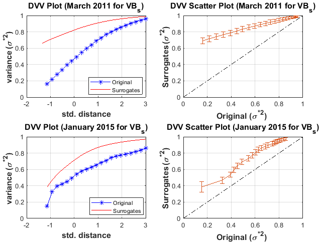
Figure 11The DVV plot and scatter plot for VBs during moderate geomagnetic storm for March 2011 and January 2015.
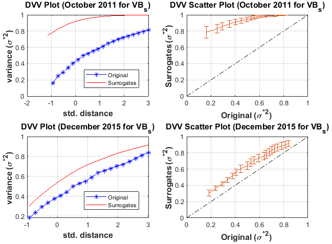
Figure 12The DVV plot and scatter plot for VBs during major geomagnetic storm for October 2011 and December 2015.
4.1 The chaotic and dynamical complexity response in Dst at minor, moderate and major geomagnetic storms
Our result shows that the values of MLE for Dst during minor geomagnetic storm are higher, indicating significant chaotic response during minor geomagnetic stormy periods (bar plot, Fig. 5). This increase in chaotic behaviour for Dst signals during minor geomagnetic storms may be as a result of asymmetry features in the longitudinal distribution of solar source region for the corotating interaction regions (CIRs) signatures responsible for the development of geomagnetic storms (Turner et al., 2006; Kozyra et al., 2006). CIR-generated magnetic storms are generally weaker than ICME- or MC-generated storms (Gonzalez et al., 1994; Tsurutani et al., 1995; Feldstein et al., 2006; Richardson and Cane, 2011). Therefore, we suspect that the increase in chaotic behaviour during minor geomagnetic storms is strongly associated with the asymmetry features in the longitudinal distribution of solar source region for the corotating interaction region (CIR) signatures. For most of these periods of moderate geomagnetic storms, the values of MLE decreases compared to minor geomagnetic storms. This revealed that as geomagnetic stormy events build up, the level of unpredictability and sensitive dependence on initial condition (chaos) begin to decrease (Lorentz, 1963; Stogaz, 1994). The chaotic behaviour during major geomagnetic storms decreases significantly compared with moderate geomagnetic storms. The reduction in chaotic response during moderate and its further declines at major geomagnetic storms may be attributed to the disturbance in the interplanetary medium driven by sheath preceding an interplanetary coronal mass ejection (ICME) or combination of the sheath and an ICME magnetic cloud (Echer et al., 2008; Tsurutani et al., 2003; Meng et al., 2019). Notably, the dynamics of the solar-wind–magnetospheric interaction are dissipative and chaotic in nature (Pavlos, 2012), and the electrodynamics of the magnetosphere due to the flux of interplanetary electric fields had a significant impact on the state of the chaotic signatures. For instance, the observation of strong chaotic behaviour during minor geomagnetic storms suggests that the dynamics was characterized by a weak magnetospheric disturbance. The reduction in chaotic behaviour at moderate and major geomagnetic storm period reveals the dynamical features with regards to when a strong magnetospheric disturbance begins to emerge. Therefore, our observation of chaotic signatures at different categories of geomagnetic storm has a potential capacity to give useful diagnostic information about monitoring space weather events. It is important to note that the features of Dst chaotic behaviour at different categories of geomagnetic storm has not been reported in the literature. For example, a previous study of Balasis et al. (2009, 2011) investigated dynamical complexity behaviour using different entropy measures and revealed the existence of low dynamical complexity in the magnetospheric dynamics and attributed it to ongoing large magnetospheric disturbance (major geomagnetic storm). The work of Balasis et al. (2009, 2011), where a certain dynamical characteristic evolved in the Dst signal was revealed, was limited to 1 year of data (2001). It is worthy to note that the year 2001, according to sunspot variations, is a period of high solar activity during solar cycle 23. It is characterized by numerous and strong solar eruptions that were followed by significant magnetic storm activities. This confirms that on most of the days in year 2001, the geomagnetic activity is strongly associated with major geomagnetic storms. The confirmation of low dynamical complexity response in the Dst signal during major geomagnetic storms agree with our current study. However, the idea of comparing the dynamical complexity behaviour at different categories of geomagnetic storms and revealing its chaotic features was not reported. This is the major reason why our present investigation is crucial to the understanding of the level of chaos and dynamical complexity involved during different categories of geomagnetic storms. As an extension to the single-year investigation done by Balasis et al. (2009, 2011) during a major geomagnetic storm, we further investigated 9 years of data of Dst that covered minor, moderate and major geomagnetic storms (see Fig. 5, stem plots) and unveiled their dynamical complexity behaviour. During major geomagnetic stormy periods, we found that the ApEn values decrease significantly, indicating reduction in the dynamical complexity behaviour. This is in agreement with the low dynamical complexity reported by Balasis et al. (2009, 2011) during a major geomagnetic period. Finally, based on the method of DVV analysis, we found that a test of non-linearity in the Dst time series during major geomagnetic storms reveals the strongest non-linearity features.
4.2 The chaotic and dynamical complexity behaviour in the VBs as input signals
The results of the MLE values for VBs revealed a strong chaotic behaviour during the three categories of geomagnetic storms. Comparing these MLE values during minor to those observed during moderate and major geomagnetic storms, the result obtained did not indicate any significant difference in chaoticity (bar plots, Fig. 6). Also, the ApEn values of VBs during the periods associated with minor, moderate and major geomagnetic storms revealed high dynamical complexity behaviour with no significant difference between the three categories of geomagnetic storms investigated. These observation of high chaotic and dynamical complexity behaviour in the dynamics of VBs may be due to interplanetary discontinuities caused by the abrupt changes in the interplanetary magnetic field direction and plasma parameters (Tsurutani et al., 2010). Also, the indication of high chaotic and dynamical complexity behaviour in VBs signifies that the solar wind electric field is stochastic in nature. The DVV analysis for VBs revealed non-linearity features with no significant difference between the minor, moderate and major geomagnetic storms. It is worth mentioning that the dynamical complexity behaviour for VBs is different from what was observed for Dst time series data. For instance, our results for Dst time series revealed that the chaotic and dynamical complexity behaviour of the magnetospheric dynamics are high during minor geomagnetic storms, reduce at moderate geomagnetic storms and further decline during major geomagnetic storms. The VBs signal revealed a high chaotic and dynamical complexity behaviour at all the categories of geomagnetic storm period. Therefore, these dynamical features obtained in the VBs as input signal and the Dst as the output in describing the magnetosphere as a non-autonomous system further support the finding of Donner et al. (2019) that found increased or unchanged behaviour in dynamical complexity for VBs and low dynamical complexity behaviour during storms using the recurrence method. This suggests that the magnetospheric dynamics are non-linear, and the solar wind dynamics are consistently stochastic in nature.
This work has examined the magnetospheric chaos and dynamical complexity behaviour in the disturbance storm time (Dst) and solar wind electric field (VBs) as input during different categories of geomagnetic storms. The chaotic and dynamical complexity behaviour at minor, moderate and major geomagnetic storms for solar wind electric field (VBs) as input and Dst as output of the magnetospheric system were analysed for the period of 9 years using non-linear dynamics tools. Our analysis has shown a noticeable trend of these non-linear parameters (MLE and ApEn) and the categories of geomagnetic storm (minor, moderate and major). The MLE and ApEn values of the Dst have indicated that the chaotic and dynamical complexity behaviour are high during minor geomagnetic storms, low during moderate geomagnetic storms and further reduced during major geomagnetic storms. The values of MLE and ApEn obtained from VBs indicate that chaotic and dynamical complexity are high with no significant difference during the periods of minor, moderate and major geomagnetic storms. Finally, the test for non-linearity in the Dst time series during major geomagnetic storms reveals the strongest non-linearity features. Based on these findings, the dynamical features obtained in the VBs as input and Dst as output of the magnetospheric system suggest that the magnetospheric dynamics are non-linear, and the solar wind dynamics are consistently stochastic in nature.
The code is a collection of routines in MATLAB (MathWorks) and is available upon request to the corresponding author.
The data of disturbance storm time (Dst) are available at the World Data Centre for Geomagnetism, Kyoto, Japan: https://doi.org/10.17593/14515-74000 (World Data Center for Geomagnetism et al., 2015), while the solar wind electric field data (VBs) are archived at the National Aeronautics and Space Administration (NASA), Space Physics Facility: https://omniweb.gsfc.nasa.gov/form/dx1.html (King and Papitashvili, 2004).
IAO analyzed the data; wrote the codes; and wrote the introduction, materials, and methods sections. OIO and OSB generated the idea behind the problem being solved and interpretation of results obtained, and OOO and ANN contributed to the discussion of the article.
The authors declare that they have no conflict of interest.
The authors would like to acknowledge the World Data Centre for Geomagnetism, Kyoto, and the National Aeronautics and Space Administration (NASA) Space Physics Facility for making the Dst data and solar wind plasma data available for research purposes. Also, the efforts of anonymous reviewers in ensuring that the quality of the work is enhanced are highly appreciated.
This paper was edited by Giovanni Lapenta and reviewed by two anonymous referees.
Akasofu, S. I.: The development of the auroral substorm, Planet. Space Sci., 12, 273–282, https://doi.org/10.1016/0032-0633(64)90151-5, 1964.
Baker, D. N. and Klimas, A. J.: The evolution of weak to strong geomagnetic activity: An interpretation in terms of deterministic chaos, J. Geophys. Res. Lett., 17, 41–44, https://doi.org/10.1029/GL017i001p00041, 1990.
Balasis, G., Daglis, I. A., Kapiris, P., Mandea, M., Vassiliadis, D., and Eftaxias, K.: From pre-storm activity to magnetic storms: a transition described in terms of fractal dynamics, Ann. Geophys., 24, 3557–3567, https://doi.org/10.5194/angeo-24-3557-2006, 2006.
Balasis, G., Daglis, I. A., Papadimitriou, C., Kalimeri, M., Anastasiadis, A., and Eftaxias, K.: Investigating dynamical complexity in the magnetosphere using various entropy measures, J. Geophys. Res., 114, A0006, https://doi.org/10.1029/2008JA014035, 2009.
Balasis, G., Daglis, I. A., Anastasiadia, A., and Eftaxias, K.: Detection of dynamical complexity changes in Dst time series using entropy concepts and rescaled range analysis, The Dynamics Magnetosphere, edited by: Liu, W. and Fujimoto, M., IAGA Special Sopron Book Series 3, Springer Science+Business Media B. V., https://doi.org/10.1007/978-94-007-0501-2_12, 2011.
Balikhin, M. A., Boynton, R. J., Billings, S. A., Gedalin, M., Ganushkina, N., and Coca, D.: Data based quest for solar wind-magnetosphere coupling function, Geophys. Res. Lett, 37, L24107, https://doi.org/10.1029/2010GL045733, 2010.
Burton, R. K., McPherron, R. L., and Russell, C. T.: An empirical relationship between interplanetary conditions and Dst, J. Geophys. Res., 80, 4204–4214, https://doi.org/10.1029/JA080i031p04204, 1975.
Consolini, G.: Emergence of dynamical complexity in the Earth's magnetosphere, in: Machine learning techniques for space weather, edited by: Camporeale, E., Wing, S., and Johnson, J. R., Elsevier, 177–202, https://doi.org/10.1016/B978-0-12-811788-0.00007-X, 2018.
Cowley, S. W. H.: The earth's magnetosphere: A brief beginner's guide, EOS Trans. Am. Geophys. Union, 76, 528–529, https://doi.org/10.1029/95EO00322, 1995.
Dessler, A. J. and Parker, E. N.: Hydromagnetic theory of magnetic storm, J. Geophys. Res, 64, 2239–2259, https://doi.org/10.1029/JZ064i012p02239, 1959.
Donner, R. V., Balasis, G., Stolbova,V., Georgiou, M., Weiderman, M., and Kurths, J.: Recurrence-based quantification of dynamical complexity in the earth's magnetosphere at geospace storm time scales, J. Geophys. Res.-Space, 124, 90–108, https://doi.org/10.1029/2018JA025318, 2019.
Dungey, J. W.: Interplanetary magnetic field and auroral zones, Phys. Rev. Lett., 6, 47–48, https://doi.org/10.1103/PhysRevLett.6.47, 1961.
Echer, E., Gonzalez, D., and Alves, M.V.: On the geomagnetic effects of solar wind interplanetary magnetic structures, Space Weather, 4, S06001, https://doi.org/10.1029/2005SW000200, 2006.
Echer, E., Gonzalez, W. D., Tsurutani, B. T., and Gonzalez, A. L. C.: Interplanetary conditions causing intense geomagnetic storms ( nT) during solar cycle 23 (1996–2006), J. Geophys. Res., 113, A05221, https://doi.org/10.1029/2007JA012744, 2008.
Feldstein, Y. I., Levitin, A. E., Kozyra, J. U., Tsurutani, B. T., Prigancova, L., Alperovich, L., Gonzalez, W. D., Mall, U., Alexeev, I. I., Gromava, L. I., and Dremukhina, L. A.: Self-consistent modelling of the large-scale distortions in the geomagnetic field during the 24–27 September 1998 major geomagnetic storm, J. Geophys. Res., 110, A11214, https://doi.org/10.1029/2004JA010584, 2005.
Feldstein, Y. I., Popov, V. A., Cumnock, J. A., Prigancova, A., Blomberg, L. G., Kozyra, J. U., Tsurutani, B. T., Gromova, L. I., and Levitin, A. E.: Auroral electrojets and boundaries of plasma domains in the magnetosphere during magnetically disturbed intervals, Ann. Geophys., 24, 2243–2276, https://doi.org/10.5194/angeo-24-2243-2006, 2006.
Fraser, A. M.: Using mutual information to estimate metric entropy, in: Dimension and Entropies in chaotic system, edited by: Mayer-Kress, G., Springer series in Synergetics, 32. Springer, Berlin, Heidelberg, 82–91, https://doi.org/10.1007/978-3-642-71001-8_11, 1986.
Fraser, A. M. and Swinney, H. L.: Independent coordinates for strange attractors from mutual information, Phys. Rev. A, 33, 1134–1140, https://doi.org/10.1103/PhysRevA.33.1134, 1986.
Gautama, T., Mandic, D. P., and Hulle, M. M. V.: The delay vector variance method for detecting determinism and nonlinearity in time series, Phys. D, 190, 167–176, https://doi.org/10.1016/j.physd.2003.11.001, 2004.
Gonzalez, W. D. and Tsurutani, B. T.: Criteria of interplanetary parameters causing intense magnetic storm ( nT), Planetary and Space Science, 35, 1101–1109, https://doi.org/10.1016/0032-0633(87)90015-8, 1987.
Gonzalez, W. D., Tsurutani, B. T., Gonalez, A. L. C., Smith, E. J., Tang, F., and Akasofu, S. I.: Solar wind-magnetosphere coupling during intense magnetic storms (1978–1979), J. Geophys. Res., 94, 8835–8851, https://doi.org/10.1029/JA094iA07p08835, 1989.
Gonzalez, W. D., Joselyn, J. A., Kamide, Y., Kroehl, H. W., Rostoker, G., Tsurutani, B. T., and Vasyliunas, V. M.: What is a geomagnetic storm?, J. Geophys. Res.-Space, 99, 5771–5792, https://doi.org/10.1029/93JA02867, 1994.
Hajra, R. and Tsurutani, B. T.: Interplanetary shocks inducing magnetospheric supersubstorms (SML < −2500 nT): unusual auroral morphologies and energy flow, Astrophys. J., 858, 123, https://doi.org/10.3847/1538-4357/aabaed, 2018.
Hajra, R., Echer, E., Tsurutani, B. T., and Gonazalez, W. D.: Solar cycle dependence of High-intensity Long-duration Continuous AE activity (HILDCAA) events, relativistic electron predictors? (2013), J. Geophys. Res.-Space, 118, 5626–5638, https://doi.org/10.1002/jgra.50530, 2013.
Imtiaz, A.: Detection of nonlinearity and stochastic nature in time series by delay vector variance method, Int. J. Eng. Tech., 10, 11–16, 2010.
Jaksic, V., Mandic, D. P., Ryan, K., Basu, B., and Pakrashi V.: A Comprehensive Study of the Delay Vector Variance Method for Quantification of Nonlinearity in dynamical Systems, R. Soc. OpenSci., 3, 150493, https://doi.org/10.1098/rsos.150493, 2016.
Johnson, J. R. and Wing, S.: A solar cycle dependence of nonlinearity in magnetospheric activity, J. Geophys. Res., 110, A04211, https://doi.org/10.1029/2004JA010638, 2005.
Kannathal, N., Choo, M. L., Acharya, U. R., and Sadasivan, P. K.: Entropies for detecting of epilepsy in EEG, Comput. Meth. Prog. Bio., 80, 187–194, https://doi.org/10.1016/j.cmpb.2005.06.012, 2005.
Kennel, M. B., Brown, R., and Abarbanel, H. D. I.: Determining embedding dimension for phase-space reconstruction using a geometrical construction, Phys. Rev. A, 45, 3403–3411, https://doi.org/10.1103/PhysRevA.45.3403, 1992.
King, J. H. and Papitashvili, N. E.: Solar wind spatial scales in and comparisons of hourly Wind and ACE plasma and magnetic field data, J. Geophys. Res., 110, A02209, https://doi.org/10.1029/2004JA010649, 2004 (data available at: https://omniweb.gsfc.nasa.gov/form/dx1.html, last access: 15 May 2021).
Klimas, A. J., Vassilliasdis, D., Baker, D. N., and Roberts, D. A.: The organized nonlinear dynamics of the magnetosphere, J. Geophys. Res., 101, 13089–13113, https://doi.org/10.1029/96JA00563, 1996.
Kozyra, J. U., Crowley, G., Emery, B. A., Fang, X., Maris, G., Mlynczak, M. G., Niciejewski, R. J., Palo, S. E., Paxton, L. J., Randall, C. E., Rong, P. P., Russell, J. M., Skinner, W., Solomon, S. C., Talaat, E. R., Wu, Q., and Yee, J. H.: Response of the Upper/Middle Atmosphere to Coronal Holes and Powerful High-Speed Solar Wind Streams in 2003, Geoph. Monog. Series, 167, 319–340, https://doi.org/10.1029/167GM24, 2006.
Kugiumtzis, D.: Test your surrogate before you test your nonlinearity, Phys. Rev. E, 60, 2808–2816, https://doi.org/10.1103/PhysRevE.60.2808, 1999.
Liou, K., Newell, P. T., Zhang, Y.-L., and Paxton, L. J.: Statistical comparison of isolated and non-isolated auroral substorms, J. Geophys. Res.-Space, 118, 2466–2477, https://doi.org/10.1002/jgra.50218, 2013.
Lorenz, E. N.: Determining nonperiodic flow, J. Atmos. Sci., 20, 130–141, https://doi.org/10.1177/0309133315623099, 1963.
Love, J. J. and Gannon, J. L.: Revised Dst and the epicycles of magnetic disturbance: 1958–2007, Ann. Geophys., 27, 3101–3131, https://doi.org/10.5194/angeo-27-3101-2009, 2009.
Mandic, D. P., Chen, M., Gautama, T., Van Hull, M. M., and Constantinides, A.: On the Characterization of the Deterministic/Stochastic and Linear/Nonlinear Nature of Time Series, Proc. R. Soc., A464, 1141–1160, https://doi.org/10.1098/rspa.2007.0154, 2007.
Mañé, R.: On the dimension of the compact invariant sets of certain nonlinear maps, in: Dynamical Systems and Turbulence, editd by: Rand, D. and Young, L. S., Warwick 1980, Springer, Berlin, Heidelberg, Lecture Notes in Mathematics, 898, 230–242, https://doi.org/10.1007/BFb0091916, 1981.
Mckinley, R. A., Mclntire, L. K., Schmidt, R., Repperger, D. W., and Caldwell, J. A.: Evaluation of Eye Metrics as a Detector of Fatigue, Human factor, 53, 403–414, https://doi.org/10.1177/0018720811411297, 2011.
Mendes, O., Domingues, M. O., Echer, E., Hajra, R., and Menconi, V. E.: Characterization of high-intensity, long-duration continuous auroral activity (HILDCAA) events using recurrence quantification analysis, Nonlin. Processes Geophys., 24, 407–417, https://doi.org/10.5194/npg-24-407-2017, 2017.
Meng, C. I., Tsurutani, B., Kawasaki, K., and Akasofu, S. I.: Cross-correlation analysis of the AE index and the interplanetary magnetic field Bz component, J. Geophys. Res., 78, 617–629, https://doi.org/10.1029/JA078i004p00617, 1973.
Meng, X., Tsurutani, B. T., and Mannucci, A. J.: The solar and interplanetary causes of superstorms (minimum nT) during the space age, J. Geophys. Res.-Space, 124, 3926–3948, https://doi.org/10.1029/2018JA026425, 2019.
Moore, C. and Marchant, T.: The approximate entropy concept extended to three dimensions for calibrated, single parameter structural complexity interrogation of volumetric images, Phys. Med. Biol., 62, 6092–6107, https://doi.org/10.1088/1361-6560/aa75b0, 2017.
Oludehinwa, I. A., Olusola, O. I., Bolaji, O. S., and Odeyemi, O. O.: Investigation of nonlinearity effect during storm time disturbance, Adv. Space. Res, 62, 440–456, https://doi.org/10.1016/j.asr.2018.04.032, 2018.
Pavlos, G. P.: The magnetospheric chaos: a new point of view of the magnetospheric dynamics. Historical evolution of magnetospheric chaos hypothesis the past two decades, Conference Proceeding of the 2nd Panhellenic Symposium, 26–29 April 1994, Democritus University, Thrace, Greece, 1994.
Pavlos, G. P.: Magnetospheric dynamics and Chaos theory, arXiv [preprint], arXiv:1203.5559, 26 March 2012.
Pavlos, G. P., Rigas, A. G., Dialetis, D., Sarris, E. T., Karakatsanis, L. P., and Tsonis, A. A.: Evidence of chaotic dynamics in the outer solar plasma and the earth magnetosphere. Chaotic dynamics: Theory and Practice, edited by: Bountis, T., Plenum Press, New York, USA, 327–339, https://doi.org/10.1007/978-1-4615-3464-8_30, 1992.
Pavlos, G. P., Athanasiu, M. A., Diamantidis, D., Rigas, A. G., and Sarris, E. T.: Comments and new results about the magnetospheric chaos hypothesis, Nonlin. Processes Geophys., 6, 99–127, https://doi.org/10.5194/npg-6-99-1999, 1999.
Pincus, S. M.: Approximate entropy as a measure of system complexity, P. Natl. Acad. Sci. USA, 88, 2297–2301, https://doi.org/10.1073/pnas.88.6.2297, 1991.
Pincus, S. M. and Goldberger, A. L.: Physiological time series analysis: what does regularity quantify, Am. J. Physiol., 266, 1643–1656, https://doi.org/10.1152/ajpheart.1994.266.4.H1643, 1994.
Pincus, S. M. and Kalman, E. K.: Irregularity, volatility, risk, and financial market time series, P. Natl. Acad. Sci. USA, 101, 13709–13714, https://doi.org/10.1073/pnas.0405168101, 2004.
Prabin Devi, S., Singh, S. B., and Surjalal Sharma, A.: Deterministic dynamics of the magnetosphere: results of the 0–1 test, Nonlin. Processes Geophys., 20, 11–18, https://doi.org/10.5194/npg-20-11-2013, 2013.
Price, C. P. and Prichard, D.: The Non-linear response of the magnetosphere: 30 October, 1978, Geophys. Res. Lett., 20, 771–774, https://doi.org/10.1029/93GL00844, 1993.
Price, C. P., Prichard, D., and Bischoff, J. E.: Nonlinear input/output analysis of the auroral electrojet index, J. Geophys. Res., 99, 13227–13238, https://doi.org/10.1029/94JA00552, 1994.
Richardson, I. G. and Cane, H. V.: Geoeffectiveness (Dst and Kp) of interplanetary coronal mass ejections during 1995–2009 and implication for storm forecasting, Space Weather, 9, S07005, https://doi.org/10.1029/2011SW000670, 2011.
Russell, C. T.: Solar wind and Interplanetary Magnetic Field: A Tutorial, Space Weather, Geophysical Monograph, 125, 73–89, https://doi.org/10.1029/GM125p0073, 2001.
Russell, C. T., McPherron, R. L., and Burton, R. K.: On the cause of geomagnetic storms, J. Geophys. Res., 79, 1105–1109, https://doi.org/10.1029/JA079i007p01105, 1974.
Shan, L.-H., Goertz, C. K., and Smith, R. A.: On the embedding-dimension analysis of AE and AL time series. Geophys. Res. Lett., 18, 1647–1650, https://doi.org/10.1029/91GL01612, 1991.
Shujuan, G. and Weidong, Z.: Nonlinear feature comparison of EEG using correlation dimension and approximate entropy, 3rd international conference on biomedical engineering and informatics, 16–18 October 2010, Yantai, China, IEEE, https://doi.org/10.1109/BMEI.2010.5639306, 2010.
Strogatz, S. H.: Nonlinear dynamics and chaos with Application to physics, Biology, chemistry and Engineering, John Wiley & Sons, New York, USA, 1994.
Sugiura, M.: Hourly Values of equatorial Dst for the IGY, Ann. Int. Geophys. Year, 35, 9–45, 1964
Sugiura, M. and Kamei T.: Equatorial Dst index 1957–1957–1986, in: IAGA bull 40. International Service of Geomagnetic Indices, edited by: Berthelier, A. and Menvielle, M., Saint-Maur-des-Fosses, France, 1991.
Takens, F.: Detecting Strange Attractors in Turbulence in Dynamical Systems, in: Dynamical systems and Turbulence, Warwick 1980. Lecture Notes in mathematics, Rand, D. and Young, L. S., Springer, Berlin, Heidelberg, vol. 898, https://doi.org/10.1007/BFb0091924, 1981.
Theiler, J., Eubank, S., Longtin, A., Galdrikian, B., and Farmer, J. D.: Testing for nonlinearity in time series: The method of surrogate data, Phys. D, 58, 77–94, https://doi.org/10.1016/0167-2789(92)90102-S, 1992.
Tsurutani, B. T. and Gonazalez, W. D.: The cause of High-intensity Long duration Continuous AE activity (HILDCAAs): Interplanetary Alfven trains, Planet. Space Sci., 35, 405–412, https://doi.org/10.1016/0032-0633(87)90097-3, 1987.
Tsurutani, B. T. and Hajra, R.: The interplanetary and magnetospheric causes of geomagnetically induced currents (GICs) > 10A in the Mantsala finland Pipeline: 1999 through 2019, J. Space Weather Space Clim., 11, 32, https://doi.org/10.1051/swsc/2021001, 2021.
Tsurutani, B. T. and Meng, C. I.: Interplanetary magnetic field variations and substorm activity, J. Geophys. Res., 77, 2964–2970, https://doi.org/10.1029/JA077i016p02964, 1972.
Tsurutani, B. T., Gonzalez, W. D., Tang, F., Akasofu, S. I., and Smith, E. J.: Origin of Interplanetary Southward Magnetic Fields Responsible for Major Magnetic Storms Near Solar Maximum (1978–1979), J. Geophys. Res., 93, 8519–8531, https://doi.org/10.1029/JA093iA08p08519, 1988.
Tsurutani, B. T., Sugiura, M., Iyemori, T., Goldstein, B. E., Gonazalez, W. D., Akasofu, S. I., and Smith, E. J.: The nonlinear response of AE to the IMF Bs driver: A spectral break at 5 hours, Geophys. Res. Lett., 17, 279–283, https://doi.org/10.1029/GL017i003p00279, 1990.
Tsurutani, B. T., Gonzalez, A. L. C., Tang, F., Arballo, J. K., and Okada, M.: Interplanetary origin of geomagnetic activity in the declining phase of the solar cycle, J. Geophys. Res., 100, 717–733, 1995.
Tsurutani, B. T., Gonzalez, W. D., Lakhina, G. S. and Alex, S.: The extreme magnetic storm of 1–2 September 1859, J. Geophys. Res., 108, 1268, https://doi.org/10.1029/2002JA009504, 2003.
Tsurutani, B. T., Lakhina, G. S., Verkhoglyadova, O. P., Gonzalez, W. D., Echer, E., and Guarnieri, F. L.: A review of interplanertary discontinuities and their geomagnetic effects, J. Atmos. Sol.-Terr. Phy., 73, 5–19, https://doi.org/10.1016/j.jastp.2010.04.001, 2010.
Tsurutani, B. T., Lakhina, G. S., and Hajra, R.: The physics of space weather/solar-terrestrial physics (STP): what we know now and what the current and future challenges are, Nonlin. Processes Geophys., 27, 75–119, https://doi.org/10.5194/npg-27-75-2020, 2020.
Tsutomu, N.: Geomagnetic storms, Journal of communications Research Laboratory, 49, 3, available at: https://www.nict.go.jp/publication/shuppan/kihou-journal/journal-vol49no3/0305.pdf (last access: 14 May 2021), 2002.
Turner, N. E., Mitchell, E. J., Knipp, D. J., and Emery, B. A.: Energetics of magnetic storms driven by corotating interaction regions: a study of geoeffectiveness, Geoph. Monog. Series, 167, 113–124, https://doi.org/10.1029/167GM11, 2006.
Unnikrishnan, K.: Comparison of chaotic aspects of magnetosphere under various physical conditions using AE index time series, Ann. Geophys., 26, 941–953, https://doi.org/10.5194/angeo-26-941-2008, 2008.
Valdivia, J. A., Sharma, A. S., and Papadopoulos, K.: Prediction of magnetic storms by nonlinear models, Geophys. Res. Lett., 23, 2899–2902, https://doi.org/10.1029/96GL02828, 1996.
Valdivia, J. A., Rogan, J., Munoz, V., Gomberoff, L., Klimas, A., Vassilliasdis, D., Uritsky, V., Sharma, S., Toledo, B., and Wastaviono, L.: The magnetosphere as a complex system, Adv. Space. Res., 35, 961–971, https://doi.org/10.1016/j.asr.2005.03.144, 2005.
Vassiliadis, D.: Systems theory for geospace plasma dynamics, Rev. Geophys., 44, RG2002, https://doi.org/10.1029/2004RG000161, 2006.
Vassilliadis, D. V., Sharma, A. S., Eastman, T. E., and Papadopoulou, K.: Low-dimensional chaos in magnetospheric activity from AE time series, J. Geophys. Res. Lett, 17, 1841–1844, https://doi.org/10.1029/GL017i011p01841, 1990.
Vassilliadis, D., Sharma, A. S., and Papadopoulos, K.: Lyapunov exponent of magnetospheric activity from AL time series, J. Geophys. Lett., 18, 1643–1646, https://doi.org/10.1029/91GL01378, 1991.
Vassiliadis, D., Klimas, A. J., Valdivia, J. A., and Baker, D. N.: The geomagnetic response as a function of storm phase and amplitude and solar wind electric field, J. Geophys. Res., 104, 24957–24976, https://doi.org/10.1029/1999JA900185, 1999.
Wallot, S. and Monster, D.: Calculation of Average Mutual Information (AMI) and False Nearest Neigbhours (FNN) for the estimation of embedding parameters of multidimensional time series in MATLAB, Front. Physchol., 9, 1679, https://doi.org/10.3389/fpsyg.2018.01679, 2018.
Wolf, A., Swift, J. B., Swinney, H. L., and Vastano, J. A.: Determining Lyapunov exponents from a time series, Phys. D, 16, 285–317, https://doi.org/10.1016/0167-2789(85)90011-9, 1985.
World Data Center for Geomagnetism, Kyoto, Nose, M., Iyemori, T., Sugiura, M., and Kamei, T.: Geomagnetic Dst index, https://doi.org/10.17593/14515-74000, 2015.
Yurchyshyn, V., Wang, H., Abramenko, V., Spirock, T., and Krucker, S.: Magnetic field, Hα and Rhessi Observations of the 2002 July 23 Gamma-ray, Astrophys. J., 605, 546–553, https://doi.org/10.1086/382142, 2004.