Identification of droughts and heatwaves in Germany with regional climate networks

Regional climate networks (RCNs) are used to identify heatwaves and droughts in Germany and two subregions for the summer half-years and summer seasons of the period 1951 to 2019. RCNs provide information for whole areas (in contrast to the point-wise information from standard indices), the underlying nodes can be distributed arbitrarily, they are easy to construct, and they provide details otherwise difficult to access, like temporal and spatial extent and localisation of extreme events; this makes them suitable for the statistical analysis of climate model output. The RCNs were constructed on the regular 0.25^∘ grid of the E-OBS data set. The season-wise correlation of the time series of daily maximum temperature T_max and precipitation were used to construct the adjacency matrix of the networks. Based on the results of a sensitivity study, we used the edge density, which increases significantly during extreme events, as the main metrics to characterise the network structure. The standard indices for comparison were the Effective Drought Index and Effective Heat Index (EDI and EHI), respectively, based on the same time series and complemented by other published data. Our results show that the RCNs are generally able to identify severe and moderate extremes and can differentiate between regions and seasons.

1 Introduction

Extreme events such as heatwaves, droughts and floods cause casualties, severe damage and economic losses. It is predicted that the frequency, duration and intensity of such extremes will increase during this century in several European regions, already affected ones, such as in the Mediterranean, and new ones in midlatitudes (Beniston et al., 2007). Knowledge about the present state and future changes in extremes is of great importance, both from the scientific perspective (process understanding) and from a societal standpoint (adaptation and mitigation measures). It would, therefore, be very useful to have a fast and easy-to-apply tool to identify extremes, vulnerable regions and critical seasons.

To identify extreme events, several extreme indices have been developed, like the Standardised Precipitation Index (SPI) for floods, the Universal Thermal Climate Index (UTCI) for heatwaves and the Palmer Drought Index (PDI) and the Effective Drought Index (EDI) for droughts, see, for instance, the World Meteorological Organization (WMO) guideline for precipitation and temperature extremes (Expert Team on Climate Change Detection and Indices – ETCCDI; http://www.wmo.int/pages/prog/wcp/wcdmp/CA_3.php, last access: 9 February 2021). These indices are used to produce catalogues of extreme events like the ones published by the European Drought Observatory (https://edo.jrc.ec.europa.eu/edov2/php/index.php?id=1000, last access: 9 February 2021). However, these indices differ considerably in purpose, timescales of interest, methods used, thresholds and, therefore, also in events considered extreme (Byun and Wilhite, 1999).

We propose here a method for identifying extremes based on regional climate networks (RCNs) which can be applied to various types of extremes, which is easy to apply and computationally efficient, which has very few tuning parameters and which permits a fast analysis for whole regions instead of single points (as do most commonly used indices). Beyond complementing existing methods, it offers several advantages. By applying the method to the results of regional climate models, present-day and future vulnerable regions can be detected. By using community detection methods and studying the temporal dynamics of the network structure (not done in this paper), the importance of processes affecting the occurrence of extremes, like weather patterns, continentality, orography and land use, can be assessed. The attribute “regional” means that the nodes of these networks are confined to a geographical region as opposed to the whole globe, similar to the difference between regional and global climate models; it is indeed our ultimate goal to apply the RCNs to the output of regional climate models to produce statistics of extreme events and/or episodes. We are interested here in extreme events happening in regions larger than a minimum size, i.e. of the order of 10 000 to 100 000 km² and are coherent and collective, i.e. most sites in such a region are affected in a similar way, so that the time series (extended over several months) of the relevant variables (daily maximum temperature and dry days) are highly correlated during extreme events; therefore, correlation coefficients above a given fixed threshold will be used to construct the RCNs in this study.

The general idea, then, of climate networks is to consider geographical points, which can be the grid points of reanalysis data, of a climate model, or a network of observation sites, as nodes of the network. A link between two nodes exists if the statistical association measure (e.g. the Pearson correlation coefficient) between the time series of the variables exceeds a given threshold. From this, one obtains the so-called adjacency matrix, which is essentially a list of connected nodes. Metrics of this adjacency matrix, like node degree, edge density and clustering coefficient, can then be used as indicators for extreme events like heatwaves, floods and droughts (see e.g. Tsonis et al., 2006).

The study of networks has evolved from graph theory; the so-called random networks were studied mathematically by Erdös and Rényi (1959). Soon after, they were recognised as a very useful tool for analysing real-world networks, like electricity grids or the internet, and for assessing their vulnerability. An overview of the networks in general and their various applications in different disciplines can be found, for example, in Newman (2003, 2019), Watts and Strogatz (1998) and Albert and Barabási (2002).

Climate networks have been increasingly used in recent years, initially mainly in a global context. They were applied to study global oscillation patterns like the El Niño–Southern Oscillation and to reveal teleconnections by Donges et al. (2009, this paper also contains definitions of higher-level network metrics). Tsonis and Swanson (2012) used climate networks to study decadal climate variability, Ludescher et al. (2013) developed a network method to improve El Niño forecasting, and Boers et al. (2014) did so for the prediction of extreme floods. It has also been shown that climate networks are able to extract interesting information about climate processes, for example, the relation between climate and topography (Peron et al., 2014). Overviews about the application of networks to climate can be found in Dijkstra et al. (2019) and the review by Franzke and O'Kane (2017). There is also an increasing number of applications of climate networks to regional scales. Rheinwalt et al. (2016) studied the spatial synchronisation of precipitation in Germany using a regional climate network. They calculated precipitation isochrones and could identify fronts along which heavy precipitation events propagated. In a similar vein, Mondal and Mishra (2021) used a regional network to analyse and predict heatwave clusters and the propagation of heatwave fronts over the United States. Weimer et al. (2016) used a regional climate network to predict future heatwaves in Europe on decadal timescales; they found that the network approach is, in some regions and decades, superior to the standard approach for estimating the occurrence of heatwaves. More applications (regional, oceanic and atmospheric studies) can be found in the overviews mentioned above.

In the present study, we use RCNs to analyse the occurrence of past heat and drought extremes in Germany and show that they have the potential to describe the occurrence frequency and spatial extent of droughts and heatwaves. Our working hypothesis is that extremes like heatwaves and droughts are characterised by spatial and temporal coherence, which is reflected in the metrics of suitably constructed regional climate networks. We will focus mainly on the edge density as being the most immediate metric, which we expect to peak for seasons in which extremes occur.

If one has such a tool, it can be integrated routinely and efficiently into the postprocessing of climate simulations to establish climatologies of extremes (specifically heatwaves and droughts) on regional scales for a given season at yearly or decadal resolution; it could also be used to routinely analyse regional climate model results (especially climate prognoses) to identify vulnerable regions, seasons prone to extremes and trends in extremes, for example. From the perspective of understanding processes, studying the structure of the adjacency matrix permits the assessment of noise factors like orography, land use, continentality and weather patterns.

This study should be considered a proof-of-concept study; we will study the sensitivity of the RCN to its construction and then apply the RCN to comparisons with present-day observations; our ultimate goal (not presented in this paper) is to apply RCNs to projections of regional climate models in various regions to assess future changes in extremes.

This paper is structured as follows: in Sect. 2, we describe the construction of networks and introduce the metrics used. We also present the data and reference extreme catalogues used, as well as the regions considered. In Sect. 3, we study the sensitivity of the network to the choice of the correlation threshold. In Sect. 4, we present comparisons of heatwaves and drought extremes identified with RCNs with standard indices and discuss the effects of chosen regions and season. A summary is given in Sect. 5.

2 Methods and data

2.1 Construction of RCNs and metrics used

We describe here only those aspects of climate networks which are relevant to our study; for more information on networks in general, the reader is referred to, for example, Newman (2003, 2019), Watts and Strogatz (1998) or Albert and Barabási (2002); climate networks are described, for example, in Tsonis et al. (2006), Dijkstra et al. (2019), Franzke and O'Kane (2017) and Donges et al. (2009). For the definition of edges, i.e. the construction of the adjacency matrix, the pairwise statistical similarity of the nodes must be quantified. For this purpose, several measures are available; frequently used ones are the Pearson correlation coefficient, event synchronisation (Boers et al., 2014) and mutual information (e.g. Franzke and O'Kane, 2017). In this study, we used the Pearson correlation coefficient ρ. We construct our RCNs, i.e. adjacency matrices, as undirected graphs with grid points of a regular longitude–latitude grid as nodes; two nodes are connected by an edge if the correlation ρ of the time series of the daily maximum temperature T_max for heatwaves and dry days for droughts, respectively, between the two nodes exceeds a predefined threshold value ρ₀. The effect of the choice of ρ₀ will be discussed in Sect. 3.

The structure of our RCN is, thus, determined by the strength of the correlation between the nodes, which has to exceed the prescribed and fixed correlation threshold, so that all metrics can vary from year to year. This approach is different from some approaches described in the literature, where the edge density is (approximately) fixed. We consider fixing the correlation threshold rather than the edge density to be more in accordance with our working hypothesis, in terms of which we expect a high and widespread correlation between the nodes during extreme seasons, which will be reflected in significant increases in the edge density and other metrics; it is the change in these metrics which will characterise extreme seasons.

In order to assess the impact of the timescales on the identification of extremes, we consider heatwaves and droughts occurring in the summer half-year (SHY; May to October) and summer season (June to August; JJA), so that the length of the time series for each year is 184 and 92 d, respectively. Although droughts are also known to occur in winter, we only consider SHY and JJA droughts here. If we denote the number of nodes by n and the edge density by e, the maximum possible number of edges is $e_{\max }=\left(\begin{array}{c}n\\ \mathrm{2}\end{array}\right)=n(n-\mathrm{1})/\mathrm{2}$. The adjacency matrix A is then an n×n matrix, with a_ij=1 if node i and node j are connected and 0 otherwise. The degree of node k, i.e. the number of nodes connected to it, will be denoted by d_k, and the average degree of the network will be denoted by $\stackrel{\mathrm{‾}}{d}$. To analyse the adjacency matrix and to identify extremes, we considered the following metrics (see, e.g., Newman, 2003 or Donges et al., 2009):

• the edge density e, defined as the number of edges in the network, divided by e_max; this can be considered a measure of the spatial extent and connection strength of the extreme event. To identify extremes, we will also use the normalised edge density, defined as $\mathit{ϵ}=(e-\stackrel{\mathrm{‾}}{e})/{\mathit{\sigma }}_e$, where $\stackrel{\mathrm{‾}}{e}$ is the average over the years 1951 to 2019, and σ_e is the corresponding standard deviation;

• the global (triangle) clustering coefficient $\stackrel{\mathrm{‾}}{c}$, defined as the average of the local clustering coefficients $c_k={\mathrm{\Delta }}_k/{\mathrm{\Delta }}_{\max ,k}$, where Δ_k is the number of triangles connected to node k, and ${\mathrm{\Delta }}_{\max ,k}=\left(\begin{array}{c}{d}_k\\ \mathrm{2}\end{array}\right)$ is the number of all triangles centred at node k (see Newman, 2003, Watts and Strogatz, 1998). Normalised values were calculated in the same way as for the edge density; and

• the distribution of the node degrees d_k, where $k=\mathrm{0}\mathrm{\dots }n-\mathrm{1}$.

We found that, in the framework of this study, these metrics and especially the edge density are sufficient for identifying extremes (see Sect. 3), and therefore, we did not consider more elaborated metrics like path length, betweenness, etc., as described, for example, in Donges et al. (2009). As already mentioned, the time series of the yearly SHY and JJA metrics were normalised by their average and standard deviation over the period 1951 to 2019; if the normalised metric of a period is larger than 1 standard deviation, this period is considered extreme; values close to 1 (about 1±0.2) are considered border cases, possibly indicating moderate, small-scale or short-lived extremes.

2.2 Data used for building the RCNs

Several time series of gridded temperature and precipitation data are freely available, for example, E-OBS (Cornes et al., 2018), ERA reanalyses (Hersbach et al., 2020) and data sets from the national weather services, for example, the German Weather Service (DWD); differences between these data sets are due to spatial and temporal resolution, observations used and statistical or interpolation methods. A comparison of such data sets can be found in (Skok et al., 2016).

In this study, we used the E-OBS V21.0e daily maximum temperature (T_max) and precipitation gridded daily data sets (https://surfobs.climate.copernicus.eu/dataaccess/access_eobs.php, last access: 9 June 2020). This data set has a spatial resolution of 0.25^∘ and covers the period from 1950 to 2019; it is updated continuously. The selected region (47–56^∘ N, 5–16^∘ E) covers Germany (henceforth called the GE region; see Fig. 6). We selected E-OBS for its relatively high resolution, its long time coverage and also for comparability due to its frequent use in other studies. Note that only data for land surfaces are provided by E-OBS. We focus here on Germany due to the high density of stations for interpolation and the availability of extreme event catalogues for comparison. For droughts, from the precipitation time series a 0–1 time series of dry days was calculated as follows: if, for a given day, the daily precipitation sum was less than 1 mm, this day was a dry day and assigned as 1; otherwise, it was assigned as 0. If their correlation coefficient exceeded a given threshold, two nodes were connected (see Sect. 4). We adopted here the E-OBS definition of a dry day as a day with a daily precipitation sum less than 1 mm d⁻¹ (see https://www.ecad.eu/FAQ/index.php#5, last access: 9 June 2020).

2.3 Identification of extreme events using the Effective Drought Index or Effective Heat Index and other sources

There exist several indices for identifying and quantifying the severity of extremes, like the Standardised Precipitation Index (SPI), Weighted Anomaly Standardized Precipitation (WASP) index, Severe Drought Index (SDI), Palmer Drought Index (PDI) and several others for drought; they differ among each other in the purpose, definition of extreme, method employed, spatial and temporal scales, focus on meteorology (precipitation) or hydrology (soil moisture and runoff); a discussion of such differences for droughts can be found in Byun and Wilhite (1999). Therefore, each choice of index is somewhat arguable and mainly determined by the need for a reference.

In this study, extreme events are identified by using spatial (over the region considered) and temporal (over the season considered) averages of the Effective Drought Index (EDI; Byun and Wilhite, 1999) and an analogous metric defined for heat, the effective heat index (EHI; Sedlmeier et al., 2016), which are basically a time series of effective temperature and precipitation, normalised by mean and standard deviation. Therefore, (relative) extremes occur when these indices deviate markedly (usually 1 standard deviation) from zero. EDI and EHI are relatively easy to calculate, use a minimum of assumptions, need no correction for trends and take the memory effect of the soil and the atmosphere into account, which is important for the assessment of the severity of heatwaves and droughts. Being aware that there is no best index, we will also have a look at other extreme event indices (see Sect. 4).

We describe here the calculation of the EDI; EHI is calculated similarly by using T_max (see Sedlmeier et al., 2016). The EDI was proposed by (Byun and Wilhite, 1999) and describes drought extremes at a site as deviations from a climatological mean state; it uses the concept of effective precipitation (EP), which takes the memory effect of the soil into account. It correlates highly with soil moisture, which makes it well suited for studying droughts.

The EP for a given day d is calculated as follows:

$$\text{EP}\left(d\right)=\sum _{k=\mathrm{1}}^{\mathrm{365}}{\mathit{\omega }}_k\cdot S_k\left(d\right),$$

where the weights are ${\mathit{\omega }}_k=\mathrm{1}/k,k=\mathrm{1},\mathrm{\dots },\mathrm{365}$ and $S_k\left(d\right)=\sum _{i=\mathrm{1}}^{k}P(d-i)$ is the precipitation sum over the last k days before day d. From EP(d), the (daily) EDI(d) is calculated, in the following, as:

$$\text{EDI}\left(d\right)=\left(\text{EP}\right(d)-\stackrel{\mathrm{‾}}{\text{EP}})/\mathit{\sigma }\left(\text{EP}\right),$$

where $\stackrel{\mathrm{‾}}{\text{EP}}$ and σ(EP) are the mean and standard deviation of EP for SHY and JJA over the period 1951 to 2019.

An analogous measure can be defined for temperature, called the EHI, with the daily maximum temperature T_max and k=49 instead of k=365 d. For the effective temperature, the value of 49 was determined as the lag where the autocorrelation function equals 0.5 (see Sedlmeier et al., 2016).

A problem in connection with EDI or EHI and many other extreme indices is that they are defined at points, whereas, for extremes, one is interested in area information. As mentioned in the introduction, this is one of the advantages of RCNs. For a comparison of the (area-wise) RCN metrics with the (point-wise) EDI and/or EHI, we calculated an areal and seasonal average of the EDI from the area-averaged effective precipitation and of the EHI from the area-averaged effective T_max; to account for the smoothing of extremes due to this averaging for a given year, season and region, we define droughts as extreme when the spatially and temporally averaged EDI is less than −1 and heat events as extreme when the spatially and temporally averaged EHI is larger than +1. We are aware that there is a certain arbitrariness in this definition. We try to reduce this arbitrariness by also considering other indices when there are large differences between EDI and/or EHI and RCN metrics or by relaxing the threshold in cases where EDI and/or EHI or RCN metrics are close to the threshold (i.e. border cases).

Valuable sources of information on the occurrence of extremes are Hannaford et al. (2011), Parry et al. (2012) and Spinoni et al. (2015). Hannaford et al. (2011) provide a detailed analysis, based on precipitation and runoff observations, of drought events (meteorological and hydrological) for several regions in Europe, among them subregions of Germany for the period 1961 to 2005. We will refer mainly to this data set to complement our comparison with EDI. For heatwaves, we will refer to Kornhuber et al. (2019), Vautard et al. (2007), Vautard et al. (2020), Zschenderlein et al. (2019), Russo et al. (2015) and Luterbacher et al. (2004).

3 Sensitivity of the metrics to correlation thresholds

The choice of the correlation threshold of the time series determines the entries of the adjacency matrix, which characterises the network and determines all metrics, like edge density, degree distribution, local and global clustering coefficient and other derived metrics; it is the only adjustable parameter in our setup of the RCN. One can either fix the correlation threshold, resulting in varying edge densities, or fix the edge density by adjusting the correlation threshold, as done, for example, in Weimer et al. (2016); both possibilities require a decision of which values to choose. We decided to use a fixed correlation threshold, since a high correlation above a fixed threshold on long (e.g. seasonal) timescales and over an extended area is an indication of a strong, persistent coupling between nodes, which is what we are looking for – we let the structure of the network reflect the given climatic situation. To see how the choice of the correlation threshold affects the metrics of the RCN, we conducted a series of sensitivity runs for drought and heat extremes. Essential criteria for judging the suitability are (i) the edge density e, which should be not to small in order to have enough data for calculating the metrics but also not too large in order to have a sufficiently large spread (e values in the literature are of the order of 0.1), and (ii) the ability of the network to detect significant differences between normal and extreme years. We varied the correlation threshold ρ₀ for ρ₀=0.70, 0.80, 0.85, 0.90, 0.95 and 0.99 for the GE region over the years 1951 to 2019. The results are now discussed separately for drought and heat.

3.1 Sensitivity droughts

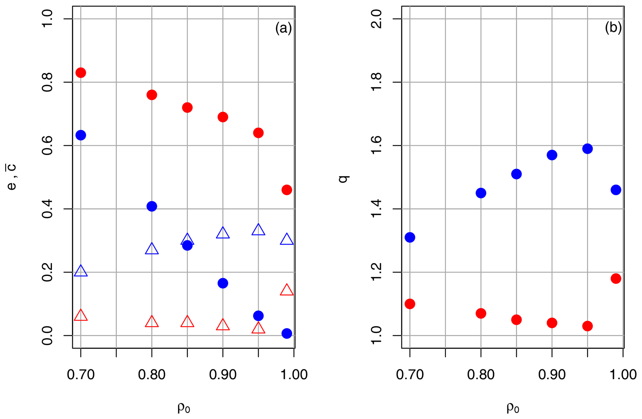
The left-hand side of Fig. 1 shows the variation in edge density e (blue circles) and global clustering coefficient $\stackrel{\mathrm{‾}}{c}$ (red circles), all averaged over the summer half-year for the years 1951 to 2019, with the correlation thresholds defined above. Also shown is the spread, i.e. ratio of the standard deviation to the average for e (blue open triangles) and $\stackrel{\mathrm{‾}}{c}$ (red open triangles) as a function of the correlation threshold.

Figure 1 Drought in the GE region in the SHY, showing the (a) average (period 1951–2019) edge density e (blue dots) and global clustering coefficient $\stackrel{\mathrm{‾}}{c}$ (red dots) as a function of the correlation threshold ρ₀ for the SHY in Germany. Also shown is the ratio of standard deviation to the average for e (blue open triangles) and $\stackrel{\mathrm{‾}}{c}$ (red open triangles) as a function of the correlation threshold. (b) The same applies for the ratio q of extreme to normal years, calculated with e (blue) and $\stackrel{\mathrm{‾}}{c}$ (red).

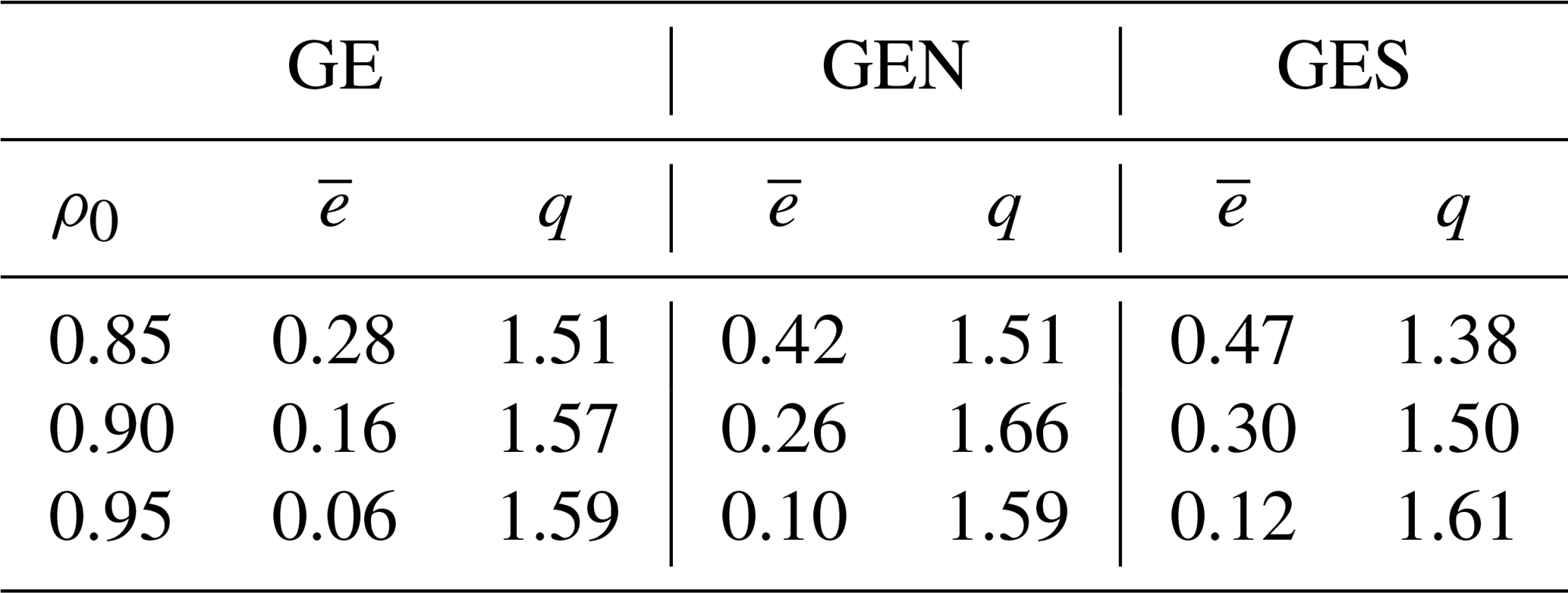
As expected, e and $\stackrel{\mathrm{‾}}{c}$ decrease considerably with increasing ρ₀; however, the sensitivity of $\stackrel{\mathrm{‾}}{c}$ is much less pronounced, although e and $\stackrel{\mathrm{‾}}{c}$ are highly correlated for all ρ₀. For ρ₀=0.70, the edge density is very high but the spread is low. The other extreme occurs for ρ₀=0.99; the spread is sufficiently large, but the values are based on too few connections, so the statistics are not reliable (for ρ₀=0.99, there are only about 90 edges out of almost 900 000 on average). For ${\mathit{\rho }}_{\mathrm{0}}=\mathrm{0.85},\mathrm{0.90}$ and 0.95, edge densities are around 0.1, which is in the range used for so-called sparse networks in the literature (Radebach et al., 2013), and the ratio of the spread to the average is around 0.5, which we consider sufficiently large.

The right-hand part of Fig. 1 shows the ratio q of the edge density (blue dots) and global clustering coefficient (red dots) averaged over extreme years (defined as years with ϵ>1) to those averaged over normal years (defined as years with $\left|\mathit{ϵ}\right|<\mathrm{0.3}$). High values of this ratio indicate that there is a significant difference between extreme and normal years, which is the ability of the RCN we are looking for. The ratio q is low for ρ₀=0.70 due to the small spread. High values above 1.6 are attained for ρ₀ in the range 0.8 to 0.95. A Wilcoxon test indicates that these differences between normal and extreme seasons are significant above the 99 % level. Concerning the global clustering coefficient $\stackrel{\mathrm{‾}}{c}$, the ratio between extreme to normal years (red dots) is only slightly above 1, i.e. it does not discriminate well between normal and extreme years, which makes it less suitable for extreme detection.

From these results, we infer that suitable values of ρ₀ for extreme drought detection are between 0.85 and 0.95, and a good separation between normal and extreme years can be achieved using the (normalised) edge density as a metric. We will use this metric and the range of ρ₀=0.85, 0.90 and 0.95 for a comparison of the RCN method with data from the literature in Sect. 4.

Table 1 shows the average and maximum degrees for ρ₀=0.85, 0.90 and 0.95 for 4 normal years (1953, 1970, 1980 and 1994) and 4 extreme years (1959, 1976, 2003 and 2018). The average degrees decrease, like the edge density (see Fig. 1), with increasing ρ₀ for normal as well as extreme years, and do not vary much between the normal years; for extreme years, the spread is larger. For all ρ₀, the average and the maximum degree increase considerably from normal to extreme years by a factor of about 2 to 3; approximately the same factor applies to the ratio maximum to average degree. Thus, the overall behaviour of the degree distributions is the same for the ρ₀ values presented and is similar within the normal and extreme year groups. The cumulative distribution of the node degrees for the GE region during the SHY is exemplarily shown in Fig. 2 for 3 normal (1953, 1970 and 1994) and 3 extreme (1959, 1976 and 2018) years, again for ρ₀=0.80, 0.90 and 0.95; for each year, the degrees are normalised with the maximum degree for better comparison. Roughly, the following two kinds of distribution can be discerned: (i) more asymmetric distributions, with either a pronounced maximum at low or high degrees (years 1953 and 2018 for ρ₀=0.95), and (ii) more symmetric (years 1976 and 1994 for ρ₀=0.85, 0.90), flat distributions, with many low-degree and high-degree nodes and a less pronounced maximum. However, there are many years which cannot be clearly attributed to either type, and both types can appear in normal and in extreme years. As Fig. 1 and Table 1 show, the main difference between normal and extreme years is the higher average (i.e. edge density) and maximum degree, which are considerably higher during extreme years.

Table 1 Drought in the GE region during the SHY, with average and maximum degrees for ρ₀=0.85, 0.90 and 0.95 for 4 normal years (1953, 1970, 1980 and 1994) and 4 extreme years (1959, 1976, 2003 and 2018).

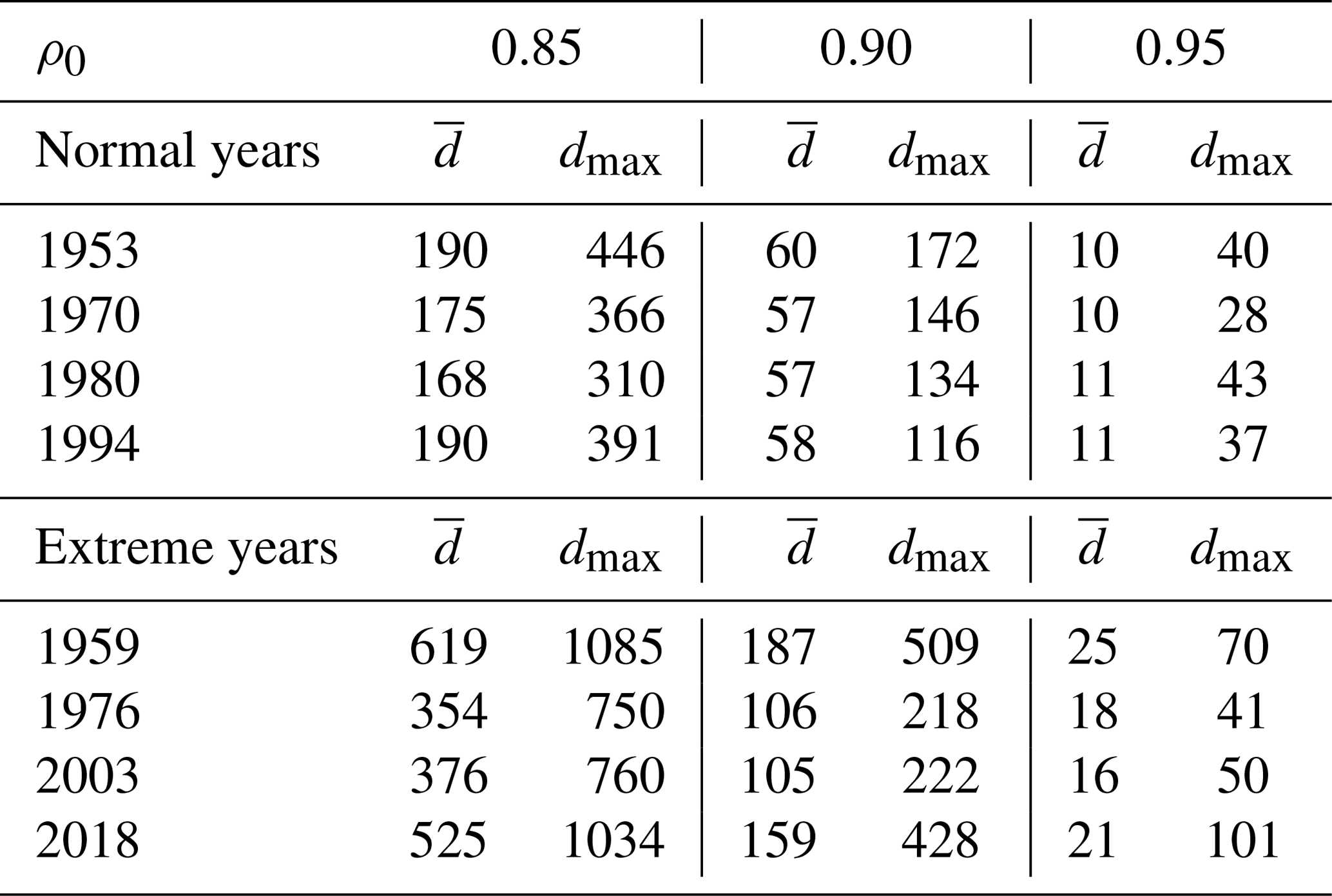
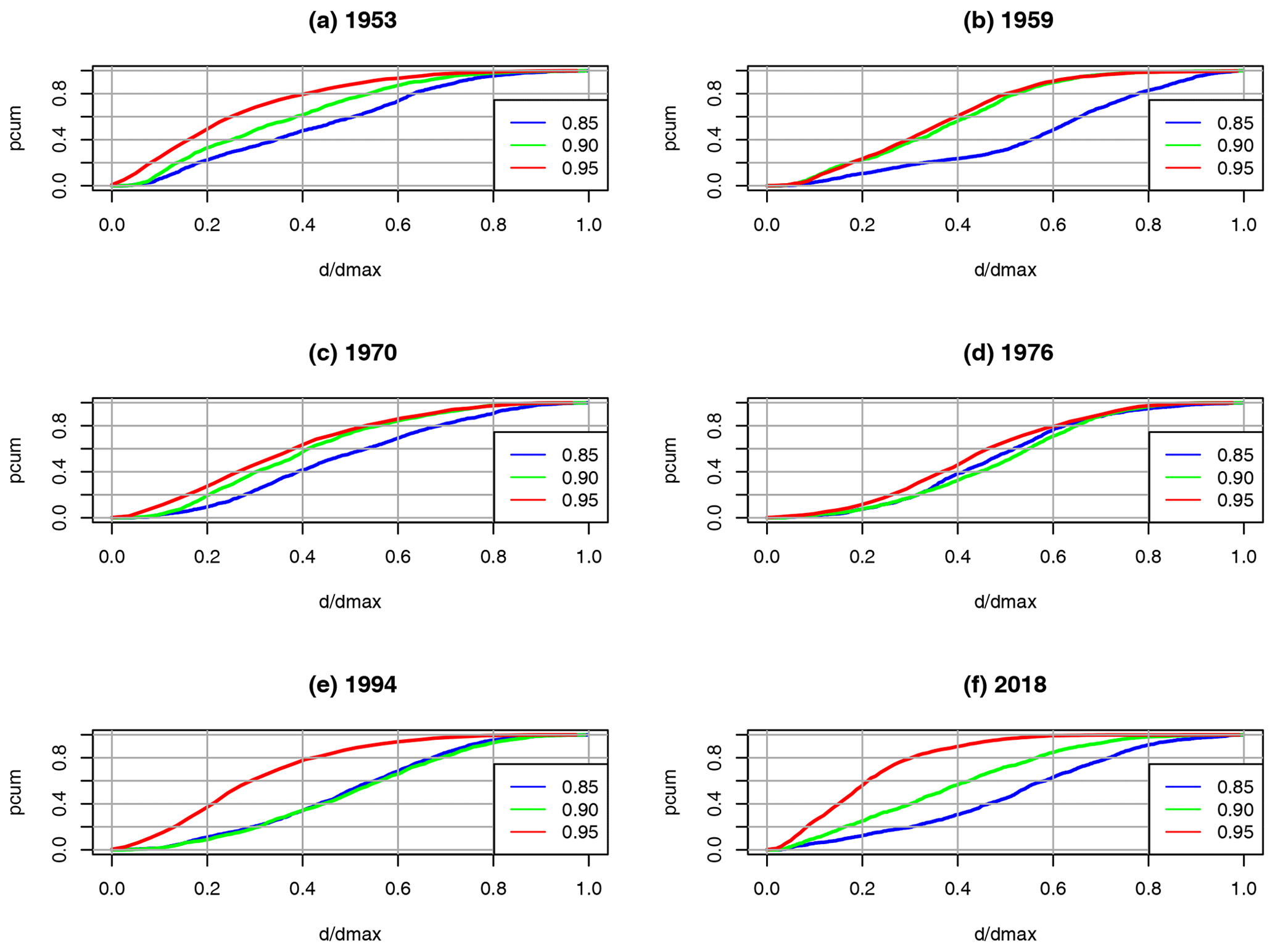
Figure 2 Drought in the GE region during the SHY, showing the dependence of the cumulative distribution p_cum on the node degrees for 3 normal (a, c, e – 1953, 1970 and 1994) and 3 extreme (b, d, f – 1959, 1976 and 2018) years on the correlation threshold ρ₀. Node degrees are normalised with maximum degree d_max.

We also found that, whereas during extreme years the distribution of the node degrees is more uniform and has more high-degree nodes, the distribution during normal years often resembles a Poisson distribution with parameter $\mathit{\lambda }=\stackrel{\mathrm{‾}}{d_k}$ (the average node degree), which is characteristic for random networks (Newman, 2003). This could be an indication of the presence of a random or, in our case, a random geometric graph (Penrose, 2003; Ferrero and Gandino, 2017). A comparison between the probability distributions for the normal year 2013 and the extreme year 2018 is shown in Fig. 3 as an example. A more Poisson-like distribution during normal years could be explained by the higher level of noise induced by the higher variability in weather systems during normal years and the presence of complex orography and varying land use, which disturb the organisation process and, thus, lead to lower correlations and lower edge densities. A detailed study to substantiate this observation is beyond the scope of this paper.

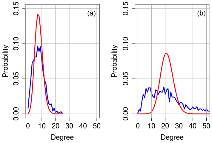
Figure 3 Node degree probability distribution for the SHY droughts in the GE region for the normal year 2013 (a) and the extreme year 2018 (b). Blue shows the distribution according to the RCN, and red shows the Poisson distribution with parameter $\mathit{\lambda }=\stackrel{\mathrm{‾}}{d_k}$ (the average node degree).

3.2 Sensitivity heatwaves

Figure 4 is the same as Fig. 1 but for heatwaves instead of droughts; the left-hand part shows the variation in edge density e and global clustering coefficient $\stackrel{\mathrm{‾}}{c}$, again averaged over the years 1951 to 2019 with the correlation threshold. We chose the summer months (JJA) here, since these months turned out to be more suitable for identifying heatwaves (see Sect. 4.2).

Figure 4 Same as Fig. 1 but for heatwaves in the GE region during JJA.

Again, the edge density and clustering coefficient decrease considerably with increasing ρ₀. Except for ρ₀=0.70, edge densities are higher than for the drought case; this could be due to the fact that correlations are higher for the continuously varying daily maximum temperatures compared to the 0–1 time series for droughts. Again, for ρ₀=0.70, edge density and clustering coefficient are high, but the spread is low, and for ρ₀=0.99, the spread is sufficiently large, but there are few connections, making the statistics unreliable. As for droughts, we calculated the ratio q of the average edge density for extreme years (defined as normalised edge density ϵ>1) to the edge density averaged over normal years (defined as $\left|\mathit{ϵ}\right|<\mathrm{0.3}$). High values around 1.5 to 1.6 are attained in the range 0.85 to 0.95. According to the Wilcoxon test, the differences between normal and extreme seasons are significant above the 99 % level. As for droughts, the ratio extreme to normal years is only slightly above 1 for the global clustering coefficient, i.e. it does not discriminate well between normal and extreme years, making it less suitable for extreme heatwave detection.

Table 2 shows the average and maximum degrees for ρ₀=0.85, 0.90 and 0.95 for 4 normal years (1975, 1991, 2005 and 2009) and 4 extreme years (1978, 2003, 2006 and 2013). The average degrees decrease, like the edge density (see Fig. 4), with increasing ρ₀ for normal and extreme years and do not vary much between the years. All values are higher than in the drought case, and the differences in normal to extreme values are smaller. For all ρ₀, the average and the maximum degree increase, from normal to extreme years, by about 50 % to 100 %; approximately the same factor applies to the ratio of the maximum to the average degree. Thus, the overall behaviour of the degree distributions is the same for the ρ₀ values presented and is similar within the normal and extreme year groups. The cumulative distribution of the node degrees for the GE region in JJA is shown exemplarily in Fig. 5 for 3 normal (1975, 1991 and 2005) and 3 extreme (1978, 2003 and 2006) years, again for ρ₀=0.80, 0.90 and 0.95. As for droughts, the following two kinds of distribution can be discerned: (i) more asymmetric distributions, with either a pronounced maximum at low or high degrees, and (ii) more symmetric, flat distributions with many low degree and high degree nodes and a less pronounced maximum. Compared to the drought case, the latter kind of distribution is the more frequent one, but still, there are many years which cannot attributed clearly to either type, and both types can appear in normal and in extreme years. As for droughts, the main difference between normal and extreme years is the higher average (i.e. edge density) and maximum degree, which are considerably higher during extreme years.

Table 2 As in Table 1 but for heatwaves in the GE region during JJA.

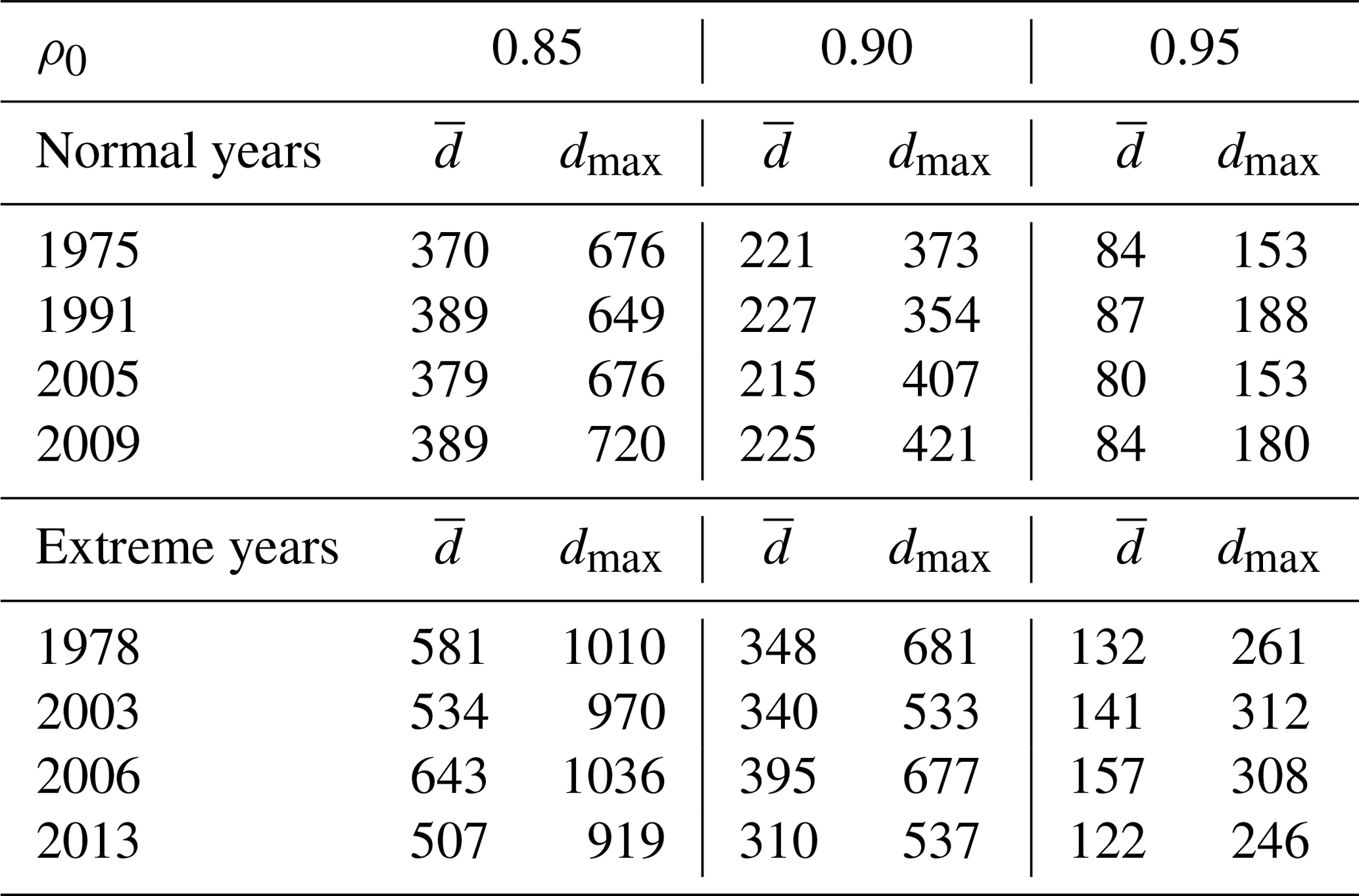
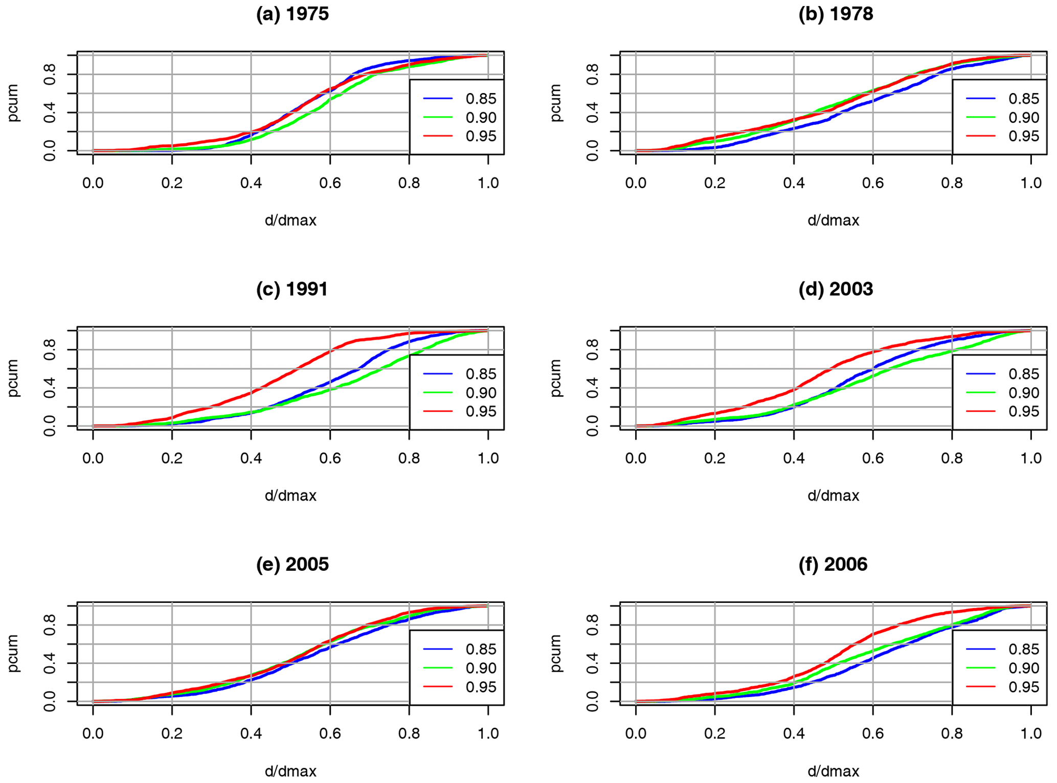
Figure 5 Same as Fig. 2 but for heatwaves in the GE region during JJA. Normal years are 1975, 1991 and 2005 (a, c, e) and extreme years are 1978, 2003 and 2006 (b, d, f).

From these findings, we conclude that, for the detection of heatwaves, suitable values of ρ₀ are between 0.85 and 0.95. This is the same range as for droughts, so, at least for heat and drought, no adjusting of the threshold ρ₀ is necessary. We will use these values in the next section, where we compare the RCN results with data from the literature.

We can summarise the findings of this sensitivity study as follows: thresholds ρ₀ between 0.85 and 0.95 give reliable results in terms of extreme detection and significance of the statistics for both drought and heatwaves. At least for these extremes, no adjusting of the threshold is necessary. The exact value of ρ₀ seems less important. Node degrees and edge densities are higher for heatwaves than for droughts. The global clustering coefficient $\stackrel{\mathrm{‾}}{c}$, although highly correlated to e for all ρ₀, does not discriminate well between extreme and normal years. In the remaining sections of this paper, we will, therefore, use the (normalised) edge density as a metric for detecting extremes and vary ρ₀ for values ρ₀=0.85, 0.90 and 0.95.

4 Comparison of the RCN results with other extreme indices (mainly EDI and EHI)

In this section, we discuss the comparison between EDI and/or EHI and RCN edge density for the summer half-years (SHYs; May to October) and summer seasons (JJA) for Germany (GE) and the two subregions, i.e. northern Germany (GEN) and southern Germany (GES), with respect to droughts and heatwaves during the period 1951–2019. EDI and EHI are averaged spatially over the respective regions and temporally over the respective season. For the reasons given in the previous section, we only consider the normalised edge density ϵ as RCN metrics. Extremes are defined as ϵ>1 for the RCN and as $\text{EDI}<-\mathrm{1}$ and EHI>1. (Note – values $\mathit{ϵ}<-\mathrm{1}$ would mean that the edge density is considerably below average; this could be caused either by wet and/or cool years or by a low correlation due to uncorrelated small-scale events. Both possibilities are not a focus of this study). For comparison, we give the results for the correlation thresholds ρ₀=0.85, 0.90 and 0.95, as discussed in the previous section. The GE, GEN and GES regions are shown in Fig. 6.

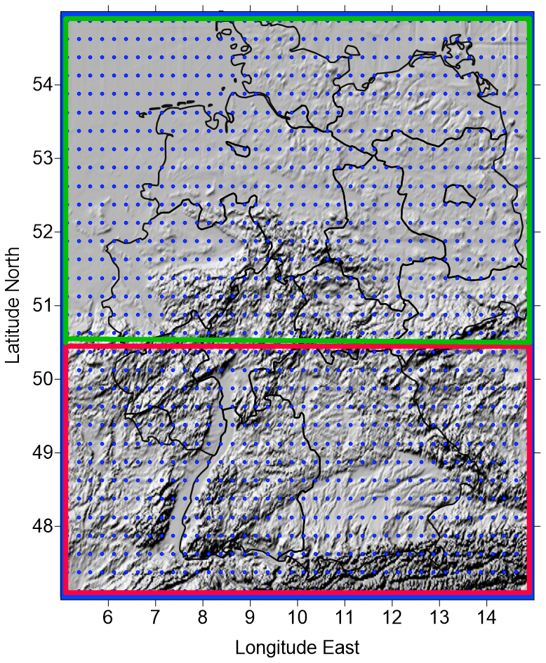
Figure 6 Relief map of Germany with the GE region (blue frame) and the subregions GES (southern Germany; red frame) and GEN (northern Germany; green frame) considered in this study. The E-OBS grid is marked by blue dots.

4.1 Droughts – GE region SHY

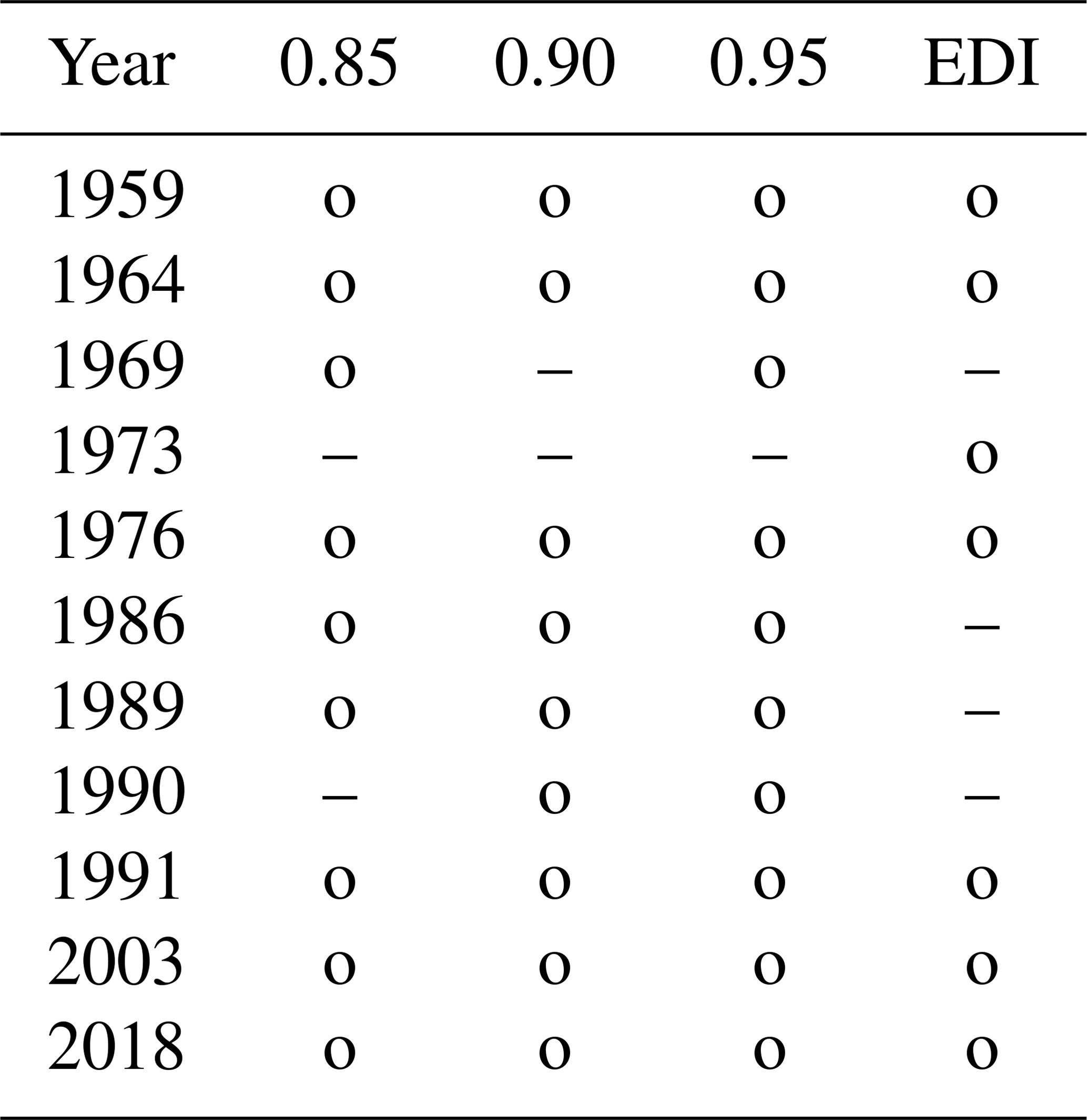
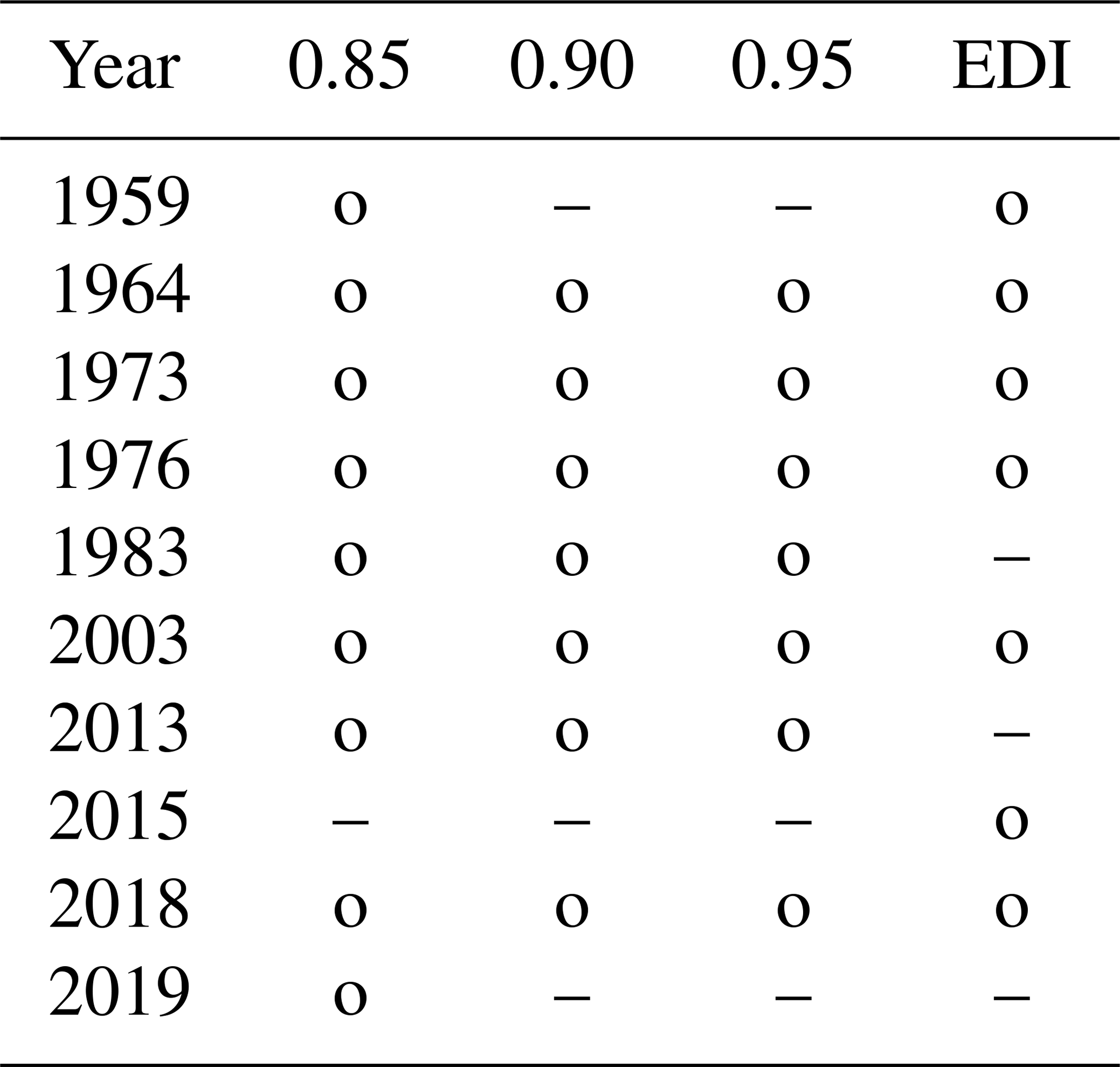
Table 3 shows the years which are identified as extreme by the RCN or by the EDI (according to the definitions above) for the SHYs over GE for the values of ρ₀ indicated above. A total of 6 years are identified by both EDI and RCN as being years with extreme droughts, namely 1959, 1964, 1976, 1991, 2003 and 2018. These years are also identified as being extreme in the literature (e.g. Spinoni et al., 2015; Hannaford et al., 2011) and the European Drought Reference (EDR) database (https://www.geo.uio.no/edc/droughtdb/edr/DroughtEvents.php, last access: 20 August 2020), so all extreme years are found by the RCN.

The year 1973, identified as being extreme by the EDI, is just below the RCN threshold of ϵ>1. The years 1969, 1986, 1989 and 1990 are not deemed extreme in EDI, whereas these years are identified as being moderately extreme in parts of Germany in Hannaford et al. (2011); the combination of the weaker signal and only regional occurrence could be a reason for the non-detection by EDI.

Thus, we can state that the RCN is able to detect the severe and moderately severe SHY drought events quoted in the literature, including less severe or only regionally severe years.

Table 3 Comparison of extreme drought summer half-years (SHYs), between 1951 and 2019, as identified by EDI and the RCN. Bars indicate SHYs identified as not extreme, and open circles indicate SHYs identified as extreme. Years according to EDI are shown in the rightmost column, and years according to the RCN, based on the normalised edge density for the correlation thresholds ρ₀=0.85, 0.90 and 0.95, are shown in columns two to four.

4.1.1 Droughts – RCN metrics differences between normal and extreme years

To illustrate the differences in the network metrics between normal and extreme years, we calculate the ratio q of the edge density averaged over extreme years between 1959 and 2019 (defined as ϵ>1) to the edge density averaged over normal years (defined as $\left|\mathit{ϵ}\right|<\mathrm{0.3}$). This ratio, together with the edge density, is shown for the GE region in the second and third column of Table 4. The edge density decreases from 0.15 to 0.01. The value of q is almost 2 for ρ₀=0.85, 0.90; this difference between extreme and normal years is significant at the 99 % level, according to a Wilcoxon test, and shows that the RCN is clearly able to differentiate between normal and extreme years.

Table 4 Dependence of the average edge density $\stackrel{\mathrm{‾}}{e}$ and the ratio $q={\stackrel{\mathrm{‾}}{e}}_{\mathrm{extr}}/{\stackrel{\mathrm{‾}}{e}}_{\mathrm{norm}}$ (edge density during extreme years to edge density during normal years) over the period 1951–2019 on the correlation threshold (ρ₀=0.85, 0.90 and 0.95). Results are shown for droughts during the SHY in the GE, GEN and GES regions.

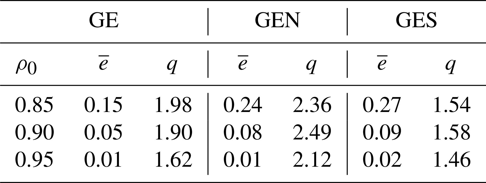
Table 4 also makes differences evident between Germany as a whole and the two subregions. All q values are quite high, with the more flat and homogeneous GEN region having generally higher values than the GES region, which is affected more by orographic noise (see the next section).

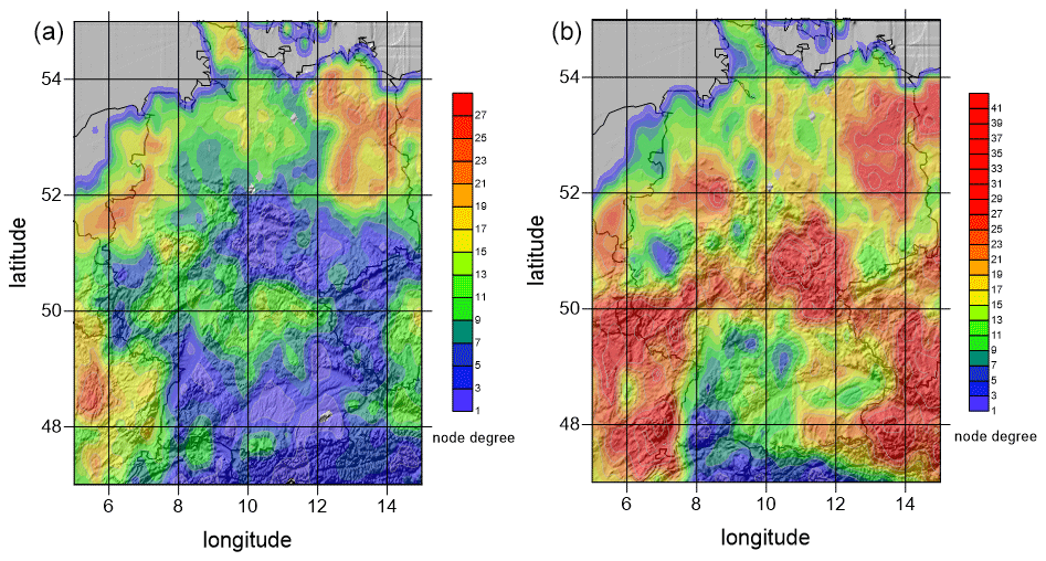
Figure 7 Comparison of the spatial distribution of the node degree between the normal year 1970 (a) and the extreme year 1976 (b). Note the different scales.

The spatial distributions of the network metrics also differ considerably between normal and extreme years. An example is shown in Fig. 7, which shows the spatial node degree distribution for the normal year 1970 (left) and the extreme year 1976 (right) for ρ₀=0.95. In 1976, average degree, maximum degree and edge density are almost double the values of 1970. Also, the following regional differences become visible: in the flat, northern parts of Germany, especially in the northeast with quite uniform sandy soils (reducing the precipitation recycling rate), node degrees tend to be considerably higher than in the more rugged, mountainous and forested southern parts ,which favour irregular precipitation distribution and, thus, act as noise in the adjacency matrix calculation. Mountainous regions are also often the ones with lower node degree in the 1976 extreme drought year; however, exceptions occur in some mountainous regions in the north and east, perhaps due to stronger impact of blocking highs, increased continentality in the east and less available moisture in the atmosphere.

4.1.2 Droughts – SHY extremes in the GEN and GES regions

To illustrate the effect of orography and the geographical situation, we compare the identified extreme years of the GEN region with the ones of the mountainous GES region of Germany (see Fig. 6). Where the GES region has a complex mountainous orography with varying land use, the GEN region is mostly flat, has a more uniform land use, with dominant sandy soils, and has a more continental climate in its eastern parts. It is known that there are differences in the occurrence and intensity of extreme droughts within Germany (see, e.g., Samaniego et al., 2013). Droughts can be quite regional and can occur in different years in the northern and northeastern parts of Germany than in the southern parts. To see if this is reflected in EDI and the RCN data, we compare the EDI and the RCN edge density ϵ for the GES and GEN subregions.

Table 5 As in Table 3 but for drought in the GEN region during the SHY.

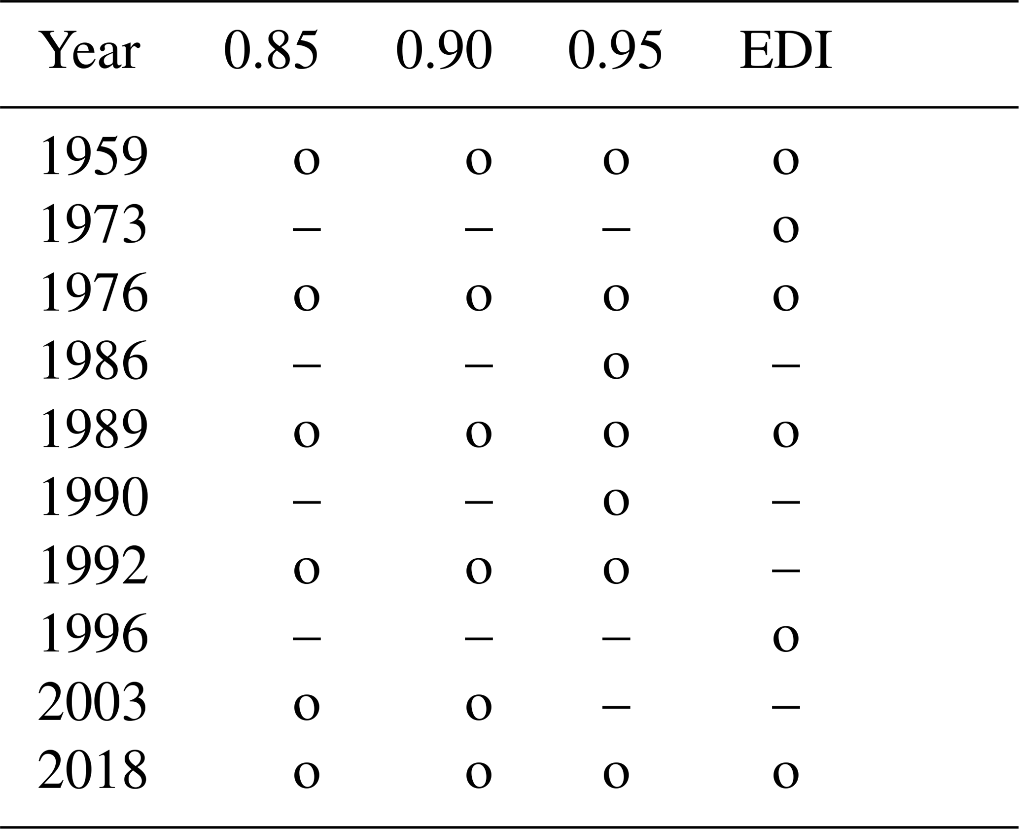
Table 6 As in Table 3 but for drought in the GES region during the SHY.

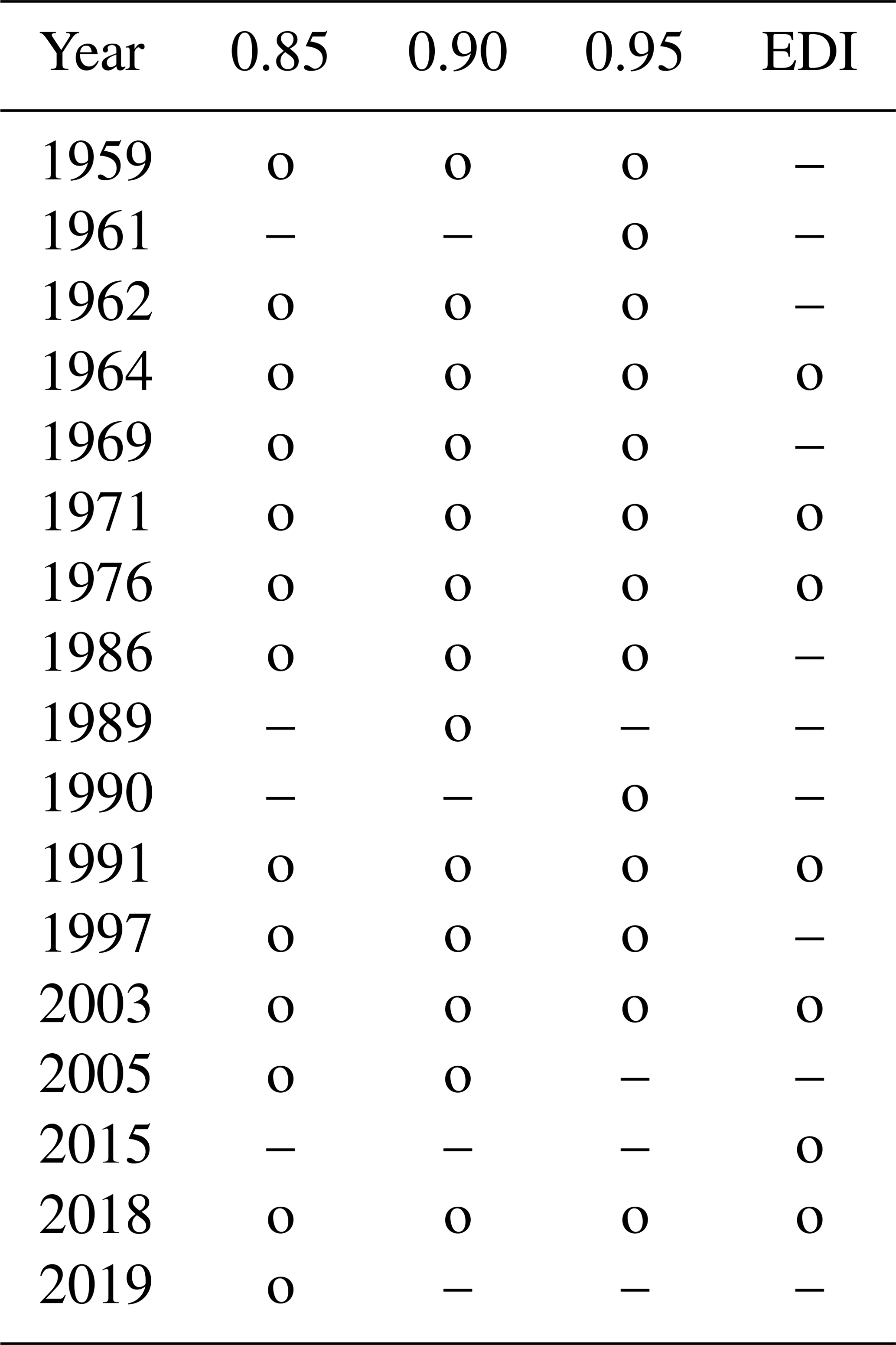
Table 5 shows the results of the RCN for the different ρ₀ and EDI for the GEN region. EDI identifies the 6 years of 1959, 1973, 1976, 1989, 1996 and 2018 as being extreme. EDI and RCN agree in the 5 years of 1959, 1976, 1989 and 2018. In the years of 1973 and 1996, the extreme years in EDI, the EDI is just below the threshold (value −1.03), so these years could be considered as border case years. On the other hand, for the years of 1992 and 2003, identified as being extreme by the RCN, the edge density is just above the threshold, so these years represent RCN border cases. In view of this, we can say that there is a very good agreement between EDI and RCN (and also with the literature) for the GEN region. The years 1964 and 1991 do not appear as extremes for the GEN region but do so for the GE region; this indicates that regional differences can be accounted for.

Table 6 shows the results for the GES region. EDI identifies the 7 years of 1964, 1971, 1976, 1991, 2003, 2015 and 2018 as being extreme. The 6 years of 1964, 1971, 1976, 1991, 2003 and 2018 are identified as being extreme years in the GES region by both RCN and EDI. The year 2015, an additional extreme year in EDI just below the threshold, is not found by the RCN. For the GES region, RCN, but not EDI, identifies the 5 years 1959, 1962, 1969, 1986 and 1997 as extreme drought years. Of these, the years 1962, 1969 and 1997 are also drought years in Hannaford et al. (2011). There are interesting differences in the occurrence of extreme years between the GES and GEN regions. For example, the year 1989, an extreme year in the GEN region, does not appear in the GES region, whereas the year 1991 is extreme in the GES region but not in the GEN region. These regional differences, which can be seen in the maps in Samaniego et al. (2013), are well captured by the RCN and indicate that the RCN is able to identify droughts at varying spatial scales. They also illustrate the fact that the spatial scales of droughts can be down to the order of 100 km.

4.1.3 Droughts – GE region during JJA

For hydrology and agriculture, it is of interest to know, on shorter timescales, when droughts are to be expected. It is also interesting to see how the RCN behaves on shorter timescales. We, therefore, compared the appearance of droughts obtained with EDI to the ones obtained by the RCN for the summer (JJA) months.

For JJA, the ratio q of extreme to normal years is above 2 and, thus, considerably higher than for the SHY (not shown). This may be due to the fact that extreme droughts occur predominantly during the JJA months and are, therefore, better captured in this shorter time window. Table 7 compares droughts derived from the RCN for JJA with the corresponding results obtained with EDI. The table again shows a good agreement between EDI and RCN. EDI identifies the 7 years of 1959, 1964, 1973, 1976, 2003, 2015 and 2018 as being extreme. Both EDI and RCN identify the 5 drought years of 1964, 1973, 1976, 2003 and 2018, so all years identified by EDI, except 1959 and 2015, are also identified by the RCN; the latter 2 years are border cases, with EDI just below −1.

Table 7 As in Table 3 but for drought in the GE region during JJA.

4.2 Heatwaves

In this section, we apply our RCN to heatwaves and compare the RCN metrics with the EHI for Germany for the summer half-year (SHY) and the summer season (JJA), respectively. As for droughts, we present the results for ρ₀=0.85, 0.90 and 0.95 and use the edge density as the relevant metric.

4.2.1 Heatwaves – GE region in the SHY

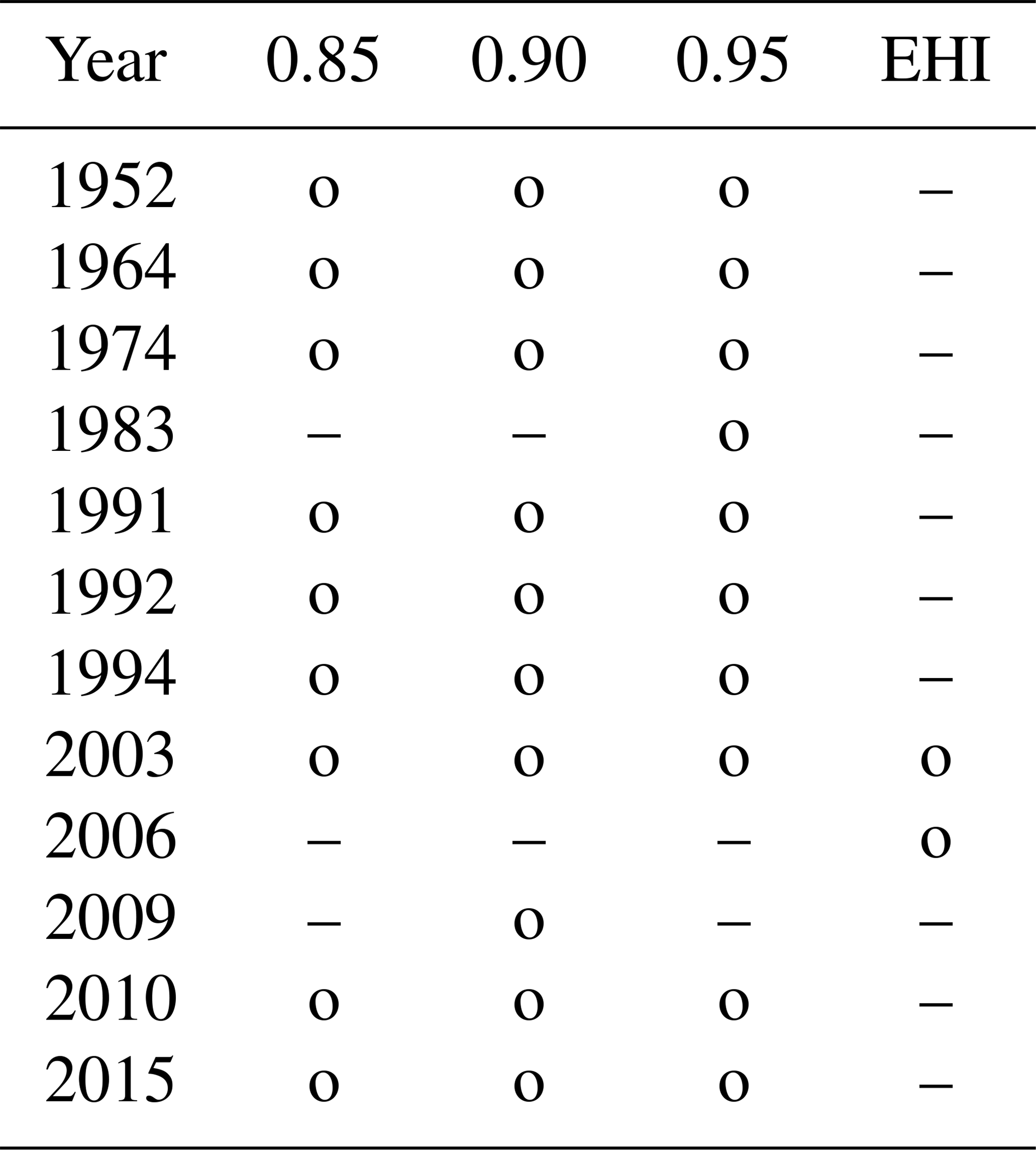
Table 8 shows the SHY years, identified as being extreme either by the RCN (ϵ>1) or by EHI (EHI>1), for the GE region and the years between 1951 and 2019. The years 2003 and 2006 are classified as extreme by the EHI, which is in line with the literature (Luterbacher et al., 2004; Russo et al., 2015), but only the year 2003 is an extreme year for RCN. In the literature, several years with extreme heat events in Germany are listed, namely 1976, 1983, 1994, 1995, 2010, 2013 and 2015 (Vautard et al., 2007, 2020; Kornhuber et al., 2019; Zschenderlein et al., 2019); these years are not identified as extreme by the EHI for the SHY, but three of them (1994, 2010 and 2015) are identified by the RCN consistently for all ρ₀ values. On the other hand, some years are identified as extreme by the RCN (1952, 1964, 1974, 1991 and 1992), which are not recorded as extreme in the literature, and the extreme year 2006 is not detected.

Table 8 As in Table 3 but for heatwaves in the GE region during the SHY.

4.2.2 Heatwaves – GE region during JJA

The results of Sect. 4.2.1 show that there are discrepancies between the heat events listed in the literature and the heat events identified by the RCN. A reason for this could be that the averaging period (SHY) is too long to identify heat events in the GE region. Thus, we look at a shorter averaging period in this section, namely JJA. As in the SHY, the metrics in JJA are highly consistent. In contrast to the SHY, the EHI identifies four severe heat events in JJA (compared to two in the SHY), namely in the years 2003, 2006, 2015 and 2018 (Table 9), in accordance with the literature (Kornhuber et al., 2019). Of these, RCN detects the years 2003 and 2006. Where the heat event of 2006 is detected in JJA, the 2015 event, detected for the SHY, is missed. The years 1983, 1994, 1995 and 2013 are identified as heat events by all thresholds of the RCN, in line with the literature (Vautard et al., 2007; Russo et al., 2015; Zschenderlein et al., 2019; Vautard et al., 2020)). However, the years 1969, 1978 and 1986 are listed as heat events by the RCN; there is no indication of these events being regionally and seasonally extended extreme events in the literature. In view of these results, we can state that shorter periods improve the detection rate (six out of eight events are detected; three events are falsely detected), but the detection rate for droughts is considerably better than the one for heatwaves. The reasons for this are not clear; since the network results are quite consistent in themselves (dependence on ρ₀; high correlation among network metrics), improvements could be achieved by changing the construction of the adjacency matrix, for example, by using different similarity measures as outlined in Sect. 3. However, such a study is beyond the scope of the present paper.

Table 9 As in Table 3 but for heatwaves in the GE region during JJA.

4.2.3 Heatwaves – RCN metric differences between normal and extreme heat years in the GE, GES and GEN regions

In order to investigate the impact of orography and the geographical situation on extreme heat events, the edge density $\stackrel{\mathrm{‾}}{e}$ and the ratio $q={\stackrel{\mathrm{‾}}{e}}_{\mathrm{extr}}/{\stackrel{\mathrm{‾}}{e}}_{\mathrm{norm}}$ (extreme versus normal years) are compared for the GE region and the GES and GEN subregions. Table 10 shows this comparison. The q values show that the edge densities increase considerably in extreme years compared to normal years, which indicates a clear separation between normal and extreme years. In contrast to droughts, there is no marked metrics difference between the GEN and GES regions. It is interesting to observe that the edge densities are larger for the subregions than for the GE region, which could be an indication of the GEN and GES regions belonging to different communities (e.g. Newman, 2019); this is, however, speculative and would require a detailed study. As already discussed in Sect. 3, heatwave edge densities are considerably higher than drought edge densities, especially in the GEN and GES subregions.

Table 10 A comparison of edge density and ratio $q={\stackrel{\mathrm{‾}}{e}}_{\mathrm{extr}}/{\stackrel{\mathrm{‾}}{e}}_{\mathrm{norm}}$ (extreme versus normal years) for the GE, GEN and GES regions and the correlation threshold ρ₀=0.85, 0.90 and 0.95 for heatwaves in JJA.

5 Summary

We used regional climate networks (RCNs) to identify heatwaves and droughts in Germany and two subregions for the summer half-years (SHYs; May–October) and summer seasons (JJA; June–August) during the period 1951 to 2019. The RCNs were constructed from maximum daily temperature and precipitation data, respectively, on the regular 0.25^∘ grid of the E-OBS data set. The season-wise correlation of the time series of these daily data was used to construct the adjacency matrix of the network. Nodes were connected by an edge if the Pearson correlation coefficient of the time series was above a fixed threshold ρ₀. Candidate metrics for identifying extremes were the edge density ϵ and the average clustering coefficient $\stackrel{\mathrm{‾}}{c}$, which turned out to be highly correlated. A sensitivity study showed that ρ₀=0.85, 0.90, and 0.95, together with the edge density as a metric, gave reasonable results. The extreme indices for comparison were the Effective Drought Index (EDI) and Effective Heat Index (EHI), respectively, based on the same time series and complemented by other published event catalogues.

Our results show that the RCNs are able to identify extremes and also to distinguish, to a certain extent, between severe and moderate events. For droughts, there is a very good agreement between EDI and RCN results. The results for heatwaves, although giving reasonable agreement, are less satisfactory than the ones for droughts; some events are not detected, while others are detected but not identified as extreme either by EHI or elsewhere in the literature. Reasons could be that some events are too local and too short lived, are centred outside the regions considered, are only in the season considered or are not intense enough. It could also be necessary to construct the adjacency matrix of the network differently either by using a different statistical association measure, for example, event synchronisation. Finding the reasons for the disagreement would require a detailed analysis of the regional and temporal temperature and precipitation conditions in the respective years, which is beyond the scope of the present paper.

Varying the size of the region considered showed that the occurrence of extreme events found by the RCN varies with the region, in accordance with observations. Furthermore, it turned out that the applicability of RCNs for identifying summertime heat events depends on the averaging period; this dependence is much less for droughts, probably due to the longer timescales. All metrics increase significantly during extreme events. Degree probability distributions vary considerably between more flat uniform ones and those with pronounced maxima but cannot be attributed to normal or extreme years. An interesting observation is that, for normal years, the distribution of the node degrees often resembles a Poisson distribution, characteristic of random networks, while for extreme years the distribution is more uniform.

There are several advantages of RCNs over conventional methods – they provide information for whole areas (in contrast to the point-wise information from standard indices) and the extent of affected areas, they can be applied to arbitrary regions, the underlying nodes can be distributed arbitrarily, they are easy to construct and they provide details otherwise difficult to access, for example, regional and seasonal differences, vulnerable regions and the impact of orography. An additional advantage of the method is that it is very fast, which makes it suitable for postprocessing climate model data. The RCN for Germany had 1338 nodes, i.e. an adjacency matrix with about 1.8 million entries; a run takes less than 4 s per year on a laptop, i.e. less than 5 min for the whole period from 1951 to 2019 when coded in Fortran 95. The algorithm could possibly be accelerated further by taking advantage of the sparsity of the adjacency matrix, since only a few percent of its entries are nonzero.

In this paper, we compared our RCN results with observations over the last 69 years in a year-to-year way, and we could show that the RCN approach yields useful information on extremes, which can complement more conventional methods. Our ultimate goal is to use the RCN method to investigate possible future changes in the frequency and seasonal distribution of extreme events in the future. For climate model projections, one can expect that the years of occurrence will vary among the models, so there is no point in year-to-year comparisons. However, our present results let us expect that statistics, e.g. over decades, can be established reliably. One of our next goals will therefore be to apply RCNs on projections of regional climate models to assess the future development of extremes and their statistics. From the application perspective, it is interesting to use other data sets to investigate the impact of the spatial resolution and size of the region considered, to apply the RCNs to other regions and to other extremes like floods and to investigate the relation of the network structure to weather patterns and orography, for example. Also, the incorporation of other relevant information as input, like soil moisture and statistics of weather patterns, could provide interesting insights.

In this proof-of-concept study, we only made use of the most basic properties of networks. Apart from improving the detection of heatwaves and other extremes as mentioned above, we also plan to look in more detail at more sophisticated metrics, degree distributions and the appearance and size of communities within the network. From a physics and climatology point of view, it is important to understand in more detail why the network measures are able to represent climate dynamics and why their success varies in order to improve the RCN method.