the Creative Commons Attribution 4.0 License.
the Creative Commons Attribution 4.0 License.
 | 25 Feb 2020
The physics of space weather/solar-terrestrial physics (STP): what we know now and what the current and future challenges are
Bruce T. Tsurutani
Gurbax S. Lakhina
Rajkumar Hajra
Major geomagnetic storms are caused by unusually intense solar wind southward magnetic fields that impinge upon the Earth's magnetosphere (Dungey, 1961). How can we predict the occurrence of future interplanetary events? Do we currently know enough of the underlying physics and do we have sufficient observations of solar wind phenomena that will impinge upon the Earth's magnetosphere? We view this as the most important challenge in space weather. We discuss the case for magnetic clouds (MCs), interplanetary sheaths upstream of interplanetary coronal mass ejections (ICMEs), corotating interaction regions (CIRs) and solar wind high-speed streams (HSSs). The sheath- and CIR-related magnetic storms will be difficult to predict and will require better knowledge of the slow solar wind and modeling to solve. For interplanetary space weather, there are challenges for understanding the fluences and spectra of solar energetic particles (SEPs). This will require better knowledge of interplanetary shock properties as they propagate and evolve going from the Sun to 1 AU (and beyond), the upstream slow solar wind and energetic “seed” particles. Dayside aurora, triggering of nightside substorms, and formation of new radiation belts can all be caused by shock and interplanetary ram pressure impingements onto the Earth's magnetosphere. The acceleration and loss of relativistic magnetospheric “killer” electrons and prompt penetrating electric fields in terms of causing positive and negative ionospheric storms are reasonably well understood, but refinements are still needed. The forecasting of extreme events (extreme shocks, extreme solar energetic particle events, and extreme geomagnetic storms (Carrington events or greater)) are also discussed. Energetic particle precipitation into the atmosphere and ozone destruction are briefly discussed. For many of the studies, the Parker Solar Probe, Solar Orbiter, Magnetospheric Multiscale Mission (MMS), Arase, and SWARM data will be useful.
- Article
(11924 KB) - Full-text XML
- BibTeX
- EndNote


1.1 Some comments on the history of the physics of space weather/solar-terrestrial physics
Space weather is a new term for a topic/science that actually began over a century and a half ago. Since everything in solar-terrestrial physics (STP) is interconnected, we think of STP as the same as space weather. It is just that with the space age beginning in 1957 (with the launch of Sputnik) and soon thereafter, many scientifically instrumented satellites led to an explosion of knowledge of the physics of space weather. However, it is useful to review some of the early scientific studies that occurred prior to 1957. Prior to the space age (where we have satellites orbiting the Earth, probing interplanetary space and viewing the Sun at UV, EUV and X-ray wavelengths), it was clearly realized that solar phenomena caused geomagnetic activity at the Earth. For example, Carrington (1859) noted that there was a magnetic storm that followed ∼17 h 40 min after the well-documented optical solar flare which he reported. This storm (Chapman and Bartels, 1940) was only more recently studied in detail by Tsurutani et al. (2003) and Lakhina et al. (2012), but the hints of a causal relationship were there in 1859. After Carrington (1959) published his seminal paper, Hale (1931), Newton (1943) and others showed that magnetic storms were delayed by several days from intense solar flares. These types of magnetic storms are now known to be caused by either their associated interplanetary coronal mass ejections (ICMEs) or their upstream sheaths. Details will be discussed later in this review.
Maunder (1904) showed that geomagnetic activity often had a ∼27 d recurrence. This periodicity was associated with some mysteriously unseen (by visible light) feature on the Sun. Chree (1905, 1913) showed that these data were statistically significant, thus inventing the Chree “superposed epoch analysis”, a scientific data analysis technique which is still used today. The mysteriously unseen solar features responsible for the geomagnetic activity were called “M-regions” by Bartels (1934), where the “M” stood for “magnetically active”. It is now known that M regions are coronal holes (Krieger et al., 1973), solar regions from which solar wind high-speed streams (HSSs) emanate, causing geomagnetic activity at the Earth (Sheeley et al., 1976, 1977; Tsurutani et al., 1995). The current status of geomagnetic activity associated with HSSs and the future work needed to better understand and to predict the various facets of space weather events will be discussed later.
With the advent of rockets and satellites, the near-Earth interplanetary medium has been probed by magnetic field, plasma, and energetic particle detectors. The Sun has been viewed at many different wavelengths. The Earth's auroral regions have recently been viewed by UV imagers, giving a global view of auroras including the dayside. The ionosphere has been probed by Global Positioning System (GPS) dual-frequency radio signals, allowing a global map of the ionospheric total electron content (TEC) at relatively high spatial and temporal resolution. The purpose of this review article will be to give a reasonably thorough review of some of the major space weather effects in the magnetosphere, ionosphere and atmosphere and in interplanetary space in order to explain what the solar and interplanetary causes are or are expected to be. The most useful part of this review will be to focus on what future advances in space weather might be in the next 10 to 25 years. In particular, we will mention which outstanding problems the Parker Solar Probe, Solar Orbiter, MMS, Arase, ICON, GOLD, and SWARM data might be useful in solving.
Our discussion will first start with phenomena that occur most frequently during solar maxima (flares, CMEs and ICME-induced magnetic storms). We will explain to the reader what is meant by an ICME and why we distinguish this from a CME. Next, phenomena associated with the declining phase of the solar cycle will be addressed. These include corotating interaction regions (CIRs) and HSSs, which cause high-intensity long-duration continuous AE activity (HILDCAA) events and the acceleration and loss of magnetospheric relativistic electrons. We will then return to the topic of interplanetary shocks and their acceleration of energetic particles in interplanetary space and also their creating new radiation belts inside the magnetosphere. Interplanetary shock impingement onto the magnetosphere create dayside auroras and also trigger nightside substorms. Prompt penetration electric fields during magnetic storm main phases will be discussed in terms of the consequences of positive and negative ionospheric storms, depending on the local time of the observation and the phase of the magnetic storm. Two relatively new topics, that of supersubstorms (SSSs) and the possibility of precipitating magnetospheric relativistic electrons affecting atmospheric weather, will be discussed. A glossary will be provided to give definitions of the terms used in this review article.
There have been some recent books and articles that touch on the many topics of the physics of space weather, though not in the same way that we will attempt to do here. We recommend for the interested reader “From the Sun: Auroras, Magnetic Storms, Solar Flares, Cosmic Rays” by Suess and Tsurutani (1998), “Magnetic Storms” by Tsurutani et al. (1997a), “Storm-Substorm Relationship” by Sharma et al. (2004), “Recurrent Magnetic Storms: Corotating Solar Wind Streams” by Tsurutani et al. (2006a), “The Sun and Space Weather” by Hanslmeier (2007), “Physics of Space Storms: From the Solar Surface to the Earth” by Koskinen (2011), and “Extreme Events in Geospace: Origins, Predictability and Consequences” by Buzulukova (2018). Because space weather is an enormous field/topic, not all facets of it have ever been covered in one book. The present authors are active researchers in the field and will attempt to introduce new viewpoints and topics not covered in the above works.
1.2 Organization of the paper
The concept of magnetic reconnection is introduced first for the non-space plasma reader. Magnetic reconnection is the physical process responsible for transferring solar wind energy into the magnetosphere during magnetic storms. We have organized the rest of the paper by discussing space weather phenomena by solar cycle intervals. However, it should be mentioned that this is not totally successful since some phenomena span all parts of the solar cycle.
Solar maximum phenomena such as CMEs, ICMEs, fast shocks, sheaths, and the forecasting of geomagnetic storms associated with the above are covered in Sects. 2.1 to 2.4. The space weather phenomena associated with the declining phase of the solar cycle are discussed in Sect. 3. Topics such as CIRs, CIR storms, HSSs, embedded Alfvén wave trains within HSSs, HILDCAA events, relativistic magnetospheric electron acceleration and loss, and electron precipitation and ozone depletion are discussed in Sects. 3.1 to 3.6. Although interplanetary shocks are primarily features associated with fast ICMEs and thus primarily a solar maximum phenomenon, shocks can also bound CIRs (∼20 % of the time) at 1 AU during the solar cycle declining phase as well. Shocks and the high-density plasmas that they create can input ram energy into the magnetosphere. Topics such as solar cosmic ray particle acceleration, dayside auroras, triggering of nightside substorms and the creation of new magnetospheric radiation belts are covered in Sects. 4.1 to 4.4. Solar flares and ionospheric TEC increases are another space weather effect causing direct solar–ionospheric coupling not involving interplanetary space or the magnetosphere. This is briefly discussed in Sect. 5. Prompt penetration electric fields (PPEFs) and ionospheric TEC increases (and decreases) occur during magnetic storms. Although the biggest effects are observed during ICME magnetic storms (solar maximum), effects have been noted in CIR magnetic storms as well. This is discussed in Sect. 6. The Carrington magnetic storm is the most intense magnetic storm in recorded history. The aurora associated with the storm reached 23∘ from the geomagnetic equator (Kimball, 1960), the lowest in recorded history. Since this event has been used as an example of extreme space weather and events of this type are a problem for U.S. Homeland Security, we felt that there should be a separate section on this topic, Sect. 7. We also discuss the possibility of events even larger than the Carrington storm occurring. In Sect. 8 auroral SSSs are discussed. Why is this topic covered in this paper? It is possible that SSSs which occur within superstorms are the actual causes of the extreme ionospheric currents, geomagnetically induced currents (GICs), that are responsible for potential power grid failures, and not the geomagnetic storms themselves. Section 9 gives our summary/conclusions for the physics and the possibility of forecasting space weather events. Section 10 is a glossary of space weather terms used by researchers in the field. Most of the definitions were carefully constructed in a previous book (Suess and Tsurutani, 1998). These should be useful for an ionospheric researcher looking up solar terms. It could be particularly useful for the non-space plasma readership as well.
2.1 Southward interplanetary magnetic fields, magnetic reconnection and magnetic storms
Figure 1 shows the Dungey (1961) scenario of magnetic reconnection. A one-to-one relationship between southward interplanetary magnetic fields (IMFs) and magnetic storms has been shown by Echer et al. (2008a) for 90 intense (Dst<−100 nT) magnetic storms that occurred during solar cycle 23. If the IMF is directed southward, it will interconnect with the Earth's magnetopause northward magnetic fields (the Earth's north magnetic pole is located in the Southern Hemisphere near the south rotational pole). The solar wind drags the interconnected magnetic fields and plasma downstream (in the antisunward direction). The open magnetic fields then reconnect in the tail. Reconnection leads to strong convection of the plasma sheet into the nightside magnetosphere.
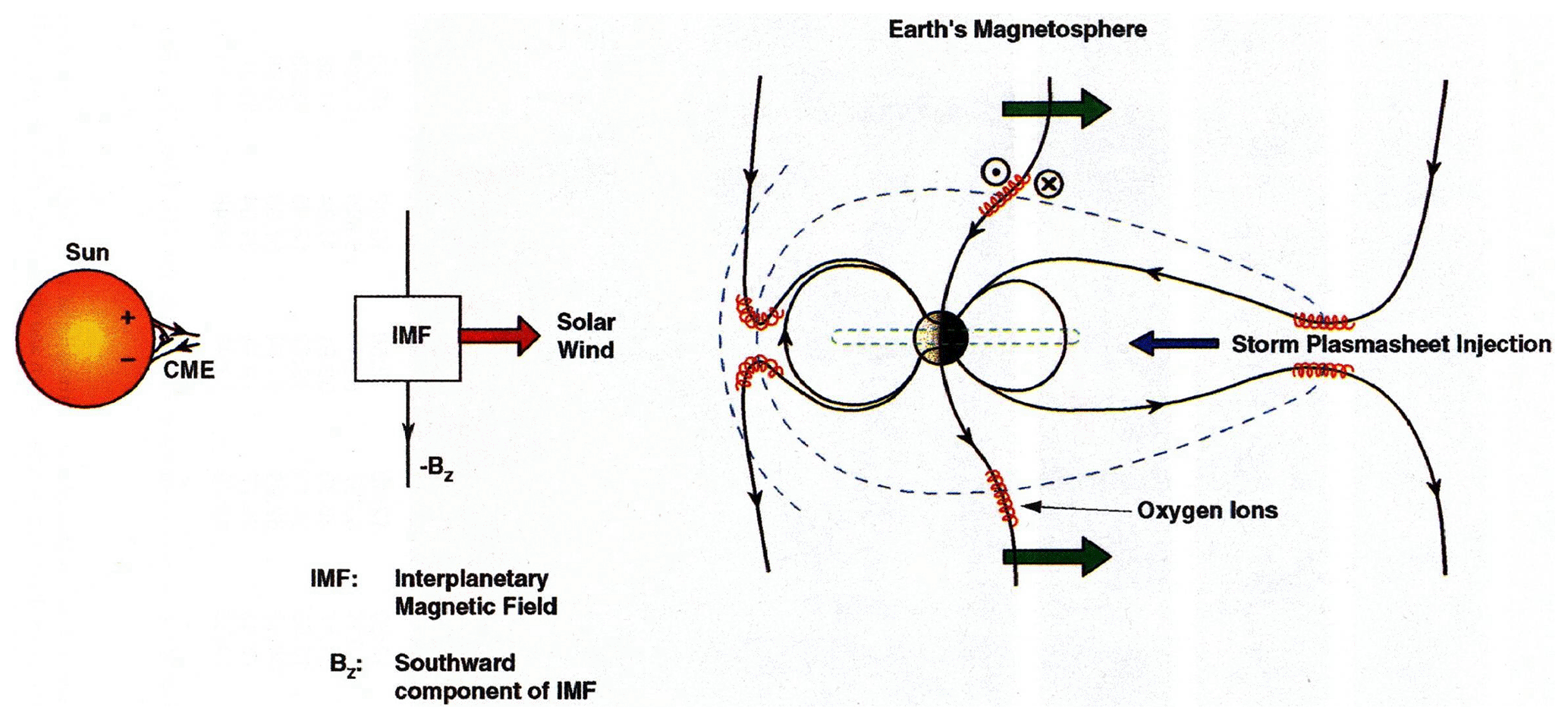
Figure 1Magnetic reconnection powering geomagnetic storms and substorms. Adapted from Dungey (1961).
What is known by theory and verified by observations is that the stronger the southward component of the IMF and the stronger the solar wind velocity convecting the magnetic field, the more strongly the solar wind–magnetospheric system is driven (e.g., Gonzalez et al., 1994). Intense IMF Bsouth in MCs (and sheaths) drives intense magnetic reconnection at the dayside magnetopause and intense reconnection on the nightside. Strong nightside magnetic reconnection leads to strong inward convection of the plasma sheet. The stronger the magnetotail reconnection, the stronger the inward convection. Via conservation of the first two adiabatic invariants (Alfvén, 1950), the greater the convection, the greater the energization of the radiation belt particles.
As the midnight sector plasma sheet is convected inward to lower L, the initially ∼100 eV to 1 keV plasma-sheet electrons and protons are adiabatically compressed (kinetically energized) so that the perpendicular (to the ambient magnetic field) energy becomes greater than the parallel energy. This leads to plasma instabilities, wave growth and wave–particle interactions (Kennel and Petschek, 1966). The resultant effect is the “diffuse aurora” caused by the precipitation of the ∼10 to 100 keV electrons and protons into the upper atmosphere/lower ionosphere. At the same time double layers are formed just above the ionosphere, giving rise to ∼1 to 10 keV “monoenergetic” electron acceleration and precipitation in the formation of “discrete auroras” (Carlson et al., 1998).
If the IMF southward component is particularly intense, this can lead to a magnetic storm with Dst<−100 nT. The Dst decrease is caused by strong convection of the plasma sheet into the inner part of the magnetosphere and the formation of an intensified ring current. This ring current produces a diamagnetic field which causes the reduced field strength at the surface of the Earth. This is the magnetic storm main phase.
After the southward field decreases or changes orientation to northward fields, the magnetic storm recovers. The recovery is associated with a multitude of physical processes associated with the loss of the energetic ring current particles: charge exchange, Coulomb collisions, wave–particle interactions and convection out the dayside magnetopause (West et al., 1972; Kozyra et al., 1997, 2006a; Jordanova et al., 1998; Daglis et al., 1999). A typical time for storm recovery is ∼10 to 24 h (Burton et al., 1975; Hamilton et al., 1988; Ebihara and Ejiri, 1998; O'Brien and McPherron, 2000; Dasso et al., 2002; Kozyra et al., 2002; Wang et al., 2003; Weygand and McPherron, 2006; Monreal MacMahon and Llop, 2008).
2.2 Coronal mass ejections (CMEs), interplanetary coronal mass ejections (ICMEs) and magnetic storms
What are the solar and interplanetary sources of intense IMFs that lead to magnetic reconnection at Earth and intense magnetic storms? What we know from space age observations is that these magnetic fields come from parts of a CME, a giant blob of plasma and magnetic fields which are released from the Sun associated with solar flares and disappearing filaments (Tang et al., 1989). Figure 2 shows the emergence of a CME from behind a solar occulting disk. The time sequence starts at the upper left, goes to the right and then to the bottom left, and ends at the bottom right. The three parts of a CME are best noted in the image on the bottom left. There is a bright outer loop most distant from the Sun, followed by a “dark region”, and then closest to the Sun is the solar filament.
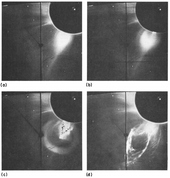
Figure 2A sequence of images showing the emergence of parts of a CME coming from the Sun. The time sequence starts at the upper left and ends at the lower right. Taken from Illing and Hundhausen (1986).
2.3 Forecasting magnetic storms and extreme storms associated with ICMEs
We will precede ourselves and state here that for the limited number of cases studied to date, the most geoeffective part of the CME is the “dark region”. Interplanetary scientists (Burlaga et al., 1981; Choe et al., 1982; Tsurutani and Gonzalez, 1994) have identified this as the low-plasma beta region called a magnetic cloud (MC), first identified by Burlaga et al. (1981) and Klein and Burlaga (1982) in interplanetary space by magnetic field and plasma measurements. When there are southward component magnetic fields within the MC (thought to typically be a giant flux rope), a magnetic storm results (Gonzalez and Tsurutani, 1987; Gonzalez et al., 1994; Tsurutani et al., 1997b; Zhang et al., 2007; Echer et al., 2008a).
It should be noted that fast CMEs and intense MC fields are relatively rare. The SOHO LASCO instrument has observed >10 000 CMEs, but only ∼5 % have speeds faster than ∼700 km s−1. Only very few have speeds >2000 km s−1, and these come from coronal regions associated with active regions (ARs) (Yashiro et al., 2004).
Interplanetary and magnetospheric scientists have developed the term ICME or interplanetary CME because it is not currently known (for individual events) how the CME evolves as it propagates from the Sun to the Earth and beyond. Leamon et al. (2004), in comparing interplanetary MCs to associated solar active regions, found that there was little or no relationship, compelling the authors to conclude that “MCs are formed during magnetic reconnection and are not simple eruptions of preexisting coronal structures”. Yurchyshyn et al. (2007) in a similar study found that “for the majority of interplanetary MCs, the fluxrope axis orientation changed less than 45∘ going from the Sun to 1 AU”. Palmerio et al. (2018) found that “for the majority of cases, the flux rope tilt angles rotated several tens of degrees (between the Sun and the Earth) while 35 % changed by more than 90∘”. Three-dimensional MHD simulations have shown that CMEs can be severely distorted as they interact with different types of interplanetary structures as they propagate through interplanetary space (Odstrcil and Pizzo, 1999a, b). The latter authors have shown that the CME distortion is substantially different when it interacts with the streamer belt (heliospheric plasma sheet/HPS) than with an HSS. The distortion of the CME can make the ICME unrecognizable at a distance further away from the Sun.
A more detailed topic not covered in Palmerio et al. (2018) or in Odstrcil and Pizzo (1999a, b) is the topic of the fate of the principal features of CMEs as discussed by Illing and Hundhausen (1986). For example, the bright outer loops are seldom identified at 1 AU (one rare case was identified by Tsurutani et al., 1998) and the filaments are typically not found within the ICME at 1 AU. The first filament detection at 1 AU was not reported until 1998 (Burlaga et al., 1998). For more recent observations of filaments at 1 AU, we direct the reader to Lepri and Zurbuchen (2010). Where have the bright outer loops and filaments gone to? Have they simply detached only to impinge onto the magnetosphere at a later time, or do they go back into the Sun? Or is it possible that many CMEs do not have filaments at their bases? Remote imaging observations from STEREO should be able to answer these questions. New in situ results from Parker Solar Probe, Solar Orbiter and ACE plus ground-based solar observations could perhaps help address the plasma physics of why typical ICMEs do not have attached filaments.
It should be remarked that the high-density solar filaments could be extremely geoeffective if they collided with the Earth's magnetosphere (this is covered later in Sect. 3.2.5). Is it possible for the MC to rotate so that initially southward magnetic fields become northward components? Can the MC fields be compressed or expanded by interplanetary interactions? Can magnetic reconnection be taking place within the ICME between the solar corona and 1 AU as suggested by Manchester et al. (2006) and Kozyra et al. (2013)? If so, how often does this occur and can it be predicted? Modeling and examining the Parker Solar Probe and Solar Orbiter data (for studies on the same ICME) could help us understand whether the MCs evolve as they propagate through interplanetary space.
Of course, the most important goal for space weather is predicting the southward magnetic fields within the ICME. This extremely difficult task is the holy grail of space weather. It is more important than predicting the time of the release of a CME, its speed and its direction.
Figure 3 shows a rare case of an ICME at 1 AU where all three parts of a CME are detected. The MC is indicated by the shaded region in the figure. The outer loop was identified by Tsurutani et al. (1998) and the filament by Burlaga et al. (1998).
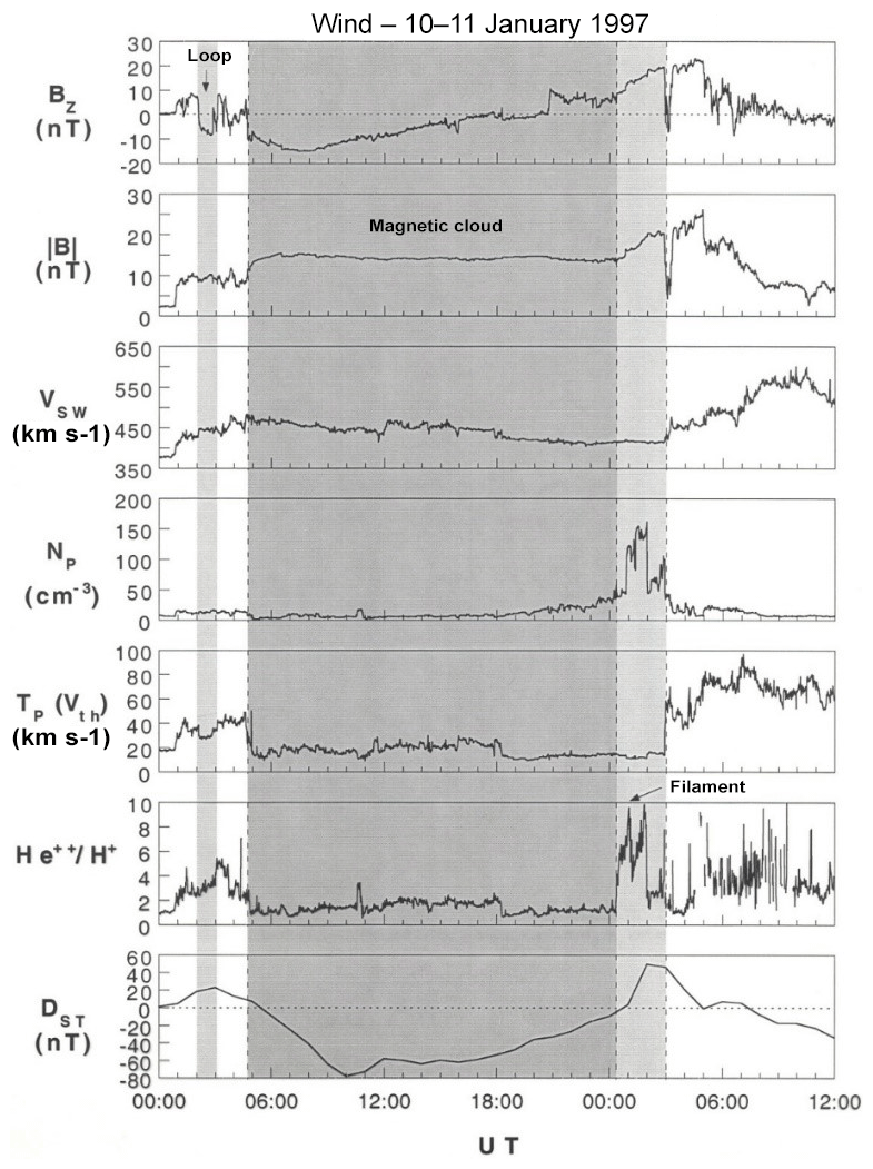
From top to bottom are the IMF Bz component (in geocentric solar magnetospheric/GSM coordinates), the field magnitude, the solar wind velocity, density, temperature and the ratio. The bottom panel gives the ground-based Dst index whose amplitude is used as an indicator of the occurrence of a magnetic storm. Dst becomes negative when the Earth's magnetosphere is filled with storm-time energetic ∼10–300 keV electrons and ions (Williams et al., 1990). Dessler and Parker (1959) and Sckopke (1966) have shown that the amount of magnetic decrease is linearly related to the total kinetic energy of the enhanced radiation belt particles. This is because the energetic particles which comprise the storm-time ring current, through gradient drift of the charged particles, form a diamagnetic current which decreases the Earth's magnetic field inside the current. We refer the reader to Sugiura (1964) and Davis and Sugiura (1966) for further discussions of the Dst index. The Dst index is a 1 h index. More recently a 1 min SYM-H index (Iyemori, 1990; Wanliss and Showalter, 2006) was developed. This is more useful for high time resolution studies. Both indices are produced by the Kyoto Data Center.
In this example (top panel of Fig. 3) the MC fields start with a strong southward (Bz<0 nT) component and then later turn northward. In the bottom panel, the magnetic storm Dst index becomes negative, with very little delay from the southward magnetic fields. The energy transfer mechanism is magnetic reconnection, as discussed earlier in Sect. 2.1. The high-density filament (fourth panel from the top) is present after the MC passage. Values as high as ∼160 cm−3 have been detected. These values are extreme values (the nominal solar wind density is ∼3 to 5 cm−3: Tsurutani et al., 2018a). The high densities impinging on the magnetosphere in this case caused compression of the magnetosphere and the Dst index to reach nT.
The stronger the southward component of the MC fields, the more intense the magnetic storm at the Earth. In extreme cases storms with intensities of Dst<−250 nT can occur (Tsurutani et al., 1992a; Echer et al., 2008b). An empirical relationship between the speed of the MC at 1 AU and its magnetic intensity has been shown by Gonzalez et al. (1998). A hypothetical explanation is the “melon seed model”: squeezing a melon seed will cause it to squirt out, and squeezing it harder will make it come out quickly. A larger magnetic field will require greater pressure to release it. However, a substantial MHD or plasma kinetic model is needed to explain the physics of this empirical relationship in more detail.
Because extremely strong MC magnetic fields are needed to produce extreme magnetic storms like the Carrington event (Tsurutani et al., 2003; Lakhina and Tsurutani, 2017), one should focus on extremely fast events for forecasting purposes. The geoeffective interplanetary dawn-to-dusk electric field is . Because Gonzalez et al. (1998) have shown that |B| is empirically proportional to Vsw, the dawn-to-dusk interplanetary electric field has a dependence. The Carrington ICME took ∼17 h 40 min to go from the Sun to Earth (Carrington, 1859), causing the largest magnetic storm in history. The minimum Dst has been estimated to be −1760 nT. However, the August 1972 event was even faster, taking only ∼14 h 40 min to go from the Sun to Earth (Vaisberg and Zastenker, 1976; Zastenker et al., 1978). Although the 1972 MC was indeed extreme in speed and magnetic field intensity, the direction of the magnetic field was northward and thus there was geomagnetic quiet following the MC impingement onto the magnetosphere (Tsurutani et al., 1992b). So again, predicting the ICME magnetic field direction is paramount in importance for space weather applications.
Modeling ICME propagation in interplanetary space during disturbed AR periods has met only limited success (Echer et al., 2009; Mostl et al., 2015; Hajra et al., 2019). Sometimes it is difficult to even identify to which flare or disappearing filament a detected ICME is related (see Tang et al., 1989). The propagation times from the Sun to 1 AU have often been in error by days (Zhao and Dryer, 2014). The additional information provided by the Parker Solar Probe and Solar Orbiter and examination of present ICME propagation codes could help improve the ability to make more accurate forecasts.
2.4 Fast shocks, sheaths and magnetic storms
Figure 4 shows a schematic of a shock and sheath upstream of an ICME. “Fast” CMEs/ICMEs can create upstream fast forward shocks (Tsurutani et al., 1988). By “fast” means that the CME/ICME is moving at a speed higher than the upstream magnetosonic (fast wave mode) speed relative to the upstream plasma and by “forward” we mean that the shock is propagating in the same direction as the “driver gas” or the CME/ICME, antisunward. When a shock is formed, it compresses the upstream plasma and magnetic fields. In this terminology, the upstream direction is the direction in which the shock is propagating (antisunward in this case) and the downstream direction is towards the Sun (see Kennel et al., 1985, and Tsurutani et al., 2011, for details on shocks). The compressed plasma and magnetic fields downstream of the shock are the “sheath”. The shock and sheath are not part of the CME/ICME. The origin of these plasma and magnetic fields is the slow solar wind altered by shock compression. This is important to understand if one wishes to predict magnetic storms caused by interplanetary sheath southward magnetic fields. It should be noted that “slow” ICMEs have been detected at 1 AU (Tsurutani et al., 1994a). These phenomena do not have upstream shocks and sheaths, as expected. However, the southward MC magnetic fields still cause magnetic storms.
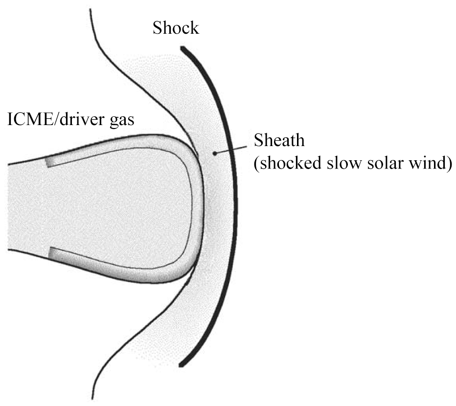
Figure 4A schematic of an interplanetary sheath antisunward of an ICME. In this diagram the Sun is on the left (not shown) (Tsurutani et al., 1988).
Kennel et al. (1985) used MHD simulations to show that the plasma densities and magnetic field magnitudes downstream of shocks are roughly related to the shock magnetosonic Mach numbers. This theoretical relationship holds up to a Mach number of ∼4. For higher Mach numbers MHD predicts that the compression will remain at a factor of ∼4. Since interplanetary shocks detected at 1 AU typically have Mach numbers only of 1 to 3 (Tsurutani and Lin, 1985; Echer et al., 2011; Meng et al., 2019), 1 to 3 are the typical shock magnetic field and density compression ratios detected at 1 AU. One question for future studies is “do the MHD relationships of magnetic field magnitude and density jumps hold for extreme shocks?” If not, there will be important consequences for extreme space weather.
Figure 5 shows a complex interplanetary event that was selected by the CAWSES II team to study in detail. The full information on this event from the Sun to the atmosphere can be found in the special issue Large Geomagnetic Storms of Solar Cycle 23 (https://agupubs.onlinelibrary.wiley.com/doi/toc/10.1002/(ISSN)1944-8007.CYCLE231, last access: 2008). What is important is that this event was associated with a solar active region (AR) and the results are quite important in terms not only of interplanetary disturbance phenomena, but also of geomagnetic activity at the Earth.
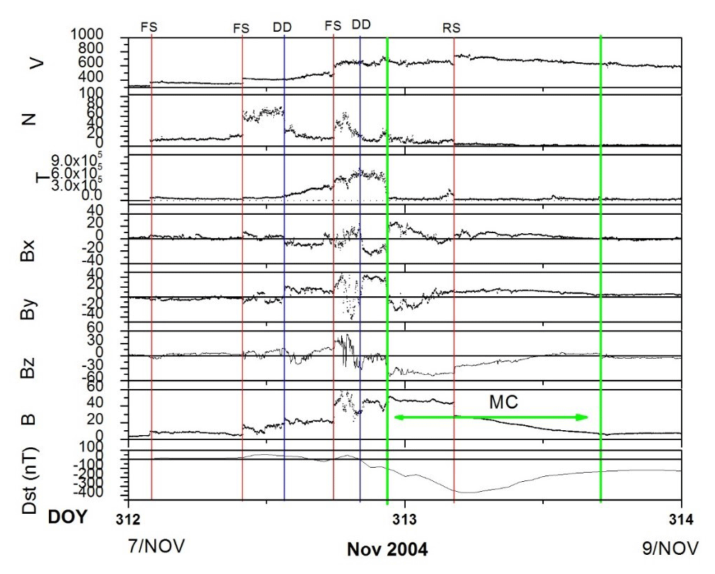
Figure 5An example of three fast forward shocks pumping up the interplanetary magnetic field intensity. Taken from Tsurutani et al. (2008a).
From top to bottom in Fig. 5 are the solar wind speed, density, and temperature, the IMF Bx, By and Bz components and the magnetic field magnitude in solar magnetospheric (GSM) coordinates. In this coordinate system, x points in the direction of the Sun, the y direction is given by , where Ω is the Earth's south magnetic pole (the south magnetic pole is near the north geographic pole), and the z axis, which is in the plane containing both the Earth–Sun line and the dipole axis, completes the right-hand side system. The magnetic storm Dst index is given at the bottom. Fast forward shocks are denoted by the three vertical red lines on 7 November 2004. There are sudden increases in the velocity, density, temperature and magnetic field magnitude at all three events. The Rankine–Hugoniot relationships have been applied to the plasma and magnetic field data and the analysis did determine that they are indeed fast shocks.
The point of showing this interplanetary event is to indicate that each shock pumps up the interplanetary sheath magnetic field by factors of ∼2 to 3. The initial magnetic field magnitude started with a value of ∼4 nT, and at the peak value after the three shocks, it reached a value of ∼60 nT. This final value was higher than the MC magnetic field, which was ∼45 nT. Details concerning the shocks and compressions can be found in the original paper for readers who are interested. What is important here is how intense interplanetary magnetic fields are created. They can come from the MCs themselves or the sheaths, as shown here. However, in this case the southward magnetic fields that caused the magnetic storm came from the MC and not the sheath.
In the above example it is believed that three fast forward shocks were associated with three ICMEs released from the AR. The longitudinal extents of shocks are, however, wider than the MCs, so only one MC was detected in the event. A similar situation was found for the August 1972 event discussed earlier.
It should be noted that a fast reverse wave (here by “reverse” we mean that the wave is propagating in the solar direction) was detected during the Fig. 5 event. It is identified as the red vertical line on 8 November. In detailed examination of the Rankine–Hugoniot conservation equations, this wave was found to propagate at a speed below the upstream magnetosonic speed, and thus was a magnetosonic wave and not a shock. This reverse wave caused a decrease in the MC magnetic field (and the southward component) and thus the start of the recovery phase of the magnetic storm. The reader should note that fast reverse waves and shocks are also important for geomagnetic activity. A detailed discussion of shock and discontinuity effects on geomagnetic activity can be found in Tsurutani et al. (2011).
Forecasting ICME sheath magnetic storms
Determination of the IMF Bz component in the sheaths will be a difficult task. To do this, more effort in understanding the slow solar wind plasma, magnetic fields and their variations will be required. To date, there has been little effort expended in this area. This is, however, easy for us to hope for, but in practice it is far more difficult to do. Use of data from Solar Probe, Solar Orbiter and a 1 AU spacecraft such as ACE could help in these analyses.
This problem has recently been emphasized by results from Meng et al. (2019). Meng et al. have shown that superstorms (Dst<−250 nT) that occurred during the space age (1957 to present) are mostly driven by sheath fields or a combination of sheath plus a following magnetic cloud (MC).
Substorms are generated by lower-intensity southward magnetic fields with the process of magnetic reconnection being the same as above. However, substorm plasma-sheet injections only go in to L∼4, the outer part of the magnetosphere (Soraas et al., 2004). The auroras associated with substorms appear in the “auroral zone”, 60 to 70∘ magnetic latitude (MLAT). Magnetic storms associated with much larger IMF Bsouth are detected at subauroral zone latitudes.
3.1 Corotating interaction region (CIR) magnetic storms
During the declining phase of the solar cycle a different type of solar and interplanetary activity dominates the physical cause of magnetic storms, that of corotating interaction regions (CIRs). HSSs emanating from coronal holes (CHs) interact with the slow solar wind and form CIRs at their interaction interfaces. The magnetic storms caused by CIRs are quite different from storms caused by ICMEs and/or their sheaths. Figure 6 shows the difference in profiles of two different types of magnetic storms. The profile of a CIR magnetic storm is shown at the bottom and that of a shock sheath ahead of an ICME MC magnetic storm on top.
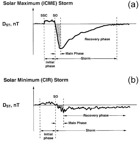
Figure 6The magnetic Dst profiles of a CIR magnetic storm (b) and an ICME magnetic storm (a). Taken from Tsurutani (2000).
The ICME MC magnetic storm Dst profile, discussed briefly earlier (see Fig. 3), is reasonably easy to identify (top panel). There is a sudden, ∼ tens of seconds' duration positive increase in Dst which is caused by the sudden increase in solar wind ram pressure due to the passage of the sheath high-density jump downstream of the shock. This compresses the magnetosphere, creating the sudden impulse (SI+: see Joselyn and Tsurutani, 1990) detected everywhere on the ground (Araki et al., 2009). Later, in either the sheath or the MC there may be a southward IMF which causes the magnetic storm. If there is a southward component in the MC, it is usually smoothly varying in intensity and direction. This leads to a smooth monotonically decreasing storm main phase as seen in the Dst index (and illustrated in Figs. 3 and 6). The loss of the ring current particles is the cause of the storm recovery phase. The details of storm recovery phase durations and causative mechanisms will be an interesting topic for magnetospheric scientists to study in the near future. The Arase mission data will be quite useful for these studies.
Figure 6b shows the typical profile of a CIR magnetic storm. It is quite different from a sheath-MC magnetic storm profile. There is no SI+ associated with the beginning of the geomagnetic disturbance. This is because CIRs detected at 1 AU typically are not led by fast forward shocks (Smith and Wolf, 1976; Tsurutani et al., 1995). The positive increase in Dst is associated with the impact of a high-density region near the heliospheric current sheet (HCS) (Smith et al., 1978; Tsurutani et al., 2006b) called the heliospheric plasma sheet (HPS; Winterhalter et al., 1994) and/or associated with the compressed plasma at the leading edge of the CIR. These are slow solar wind plasma densities. The most distinguishing feature of the CIR storm main phase is the lack of smoothness, in sharp contrast to the MC magnetic storm. This irregular Dst storm main phase is caused by large Bz fluctuations within the CIR.
CIR magnetic fields have magnitudes of ∼20 to 30 nT and typically do not reach the much higher intensities that MC fields typically do. For this reason and also because of the IMF Bz fluctuations, CIR magnetic storms usually have intensities nT (small or no magnetic storms). Extreme magnetic storms with Dst<−250 nT caused by CIRs are rare, if they occur at all (none were found in the Meng et al., 2019, study). However, it is clear that compound events involving both CIRs, sheaths ahead of ICMEs and ICMEs could certainly cause extreme magnetic storm events.
CIR-related magnetic storms occur most frequently during the declining phase of the solar cycle, and ICME magnetic storms typically occur near the maximum phase of the solar cycle. However, it should be noted that both CIR storms and sheath and/or ICME MC magnetic storms can occur during any phase of the solar cycle. We have simply ordered things by solar cycle so that it will be easier to give the reader the general picture of space weather.
3.2 Coronal holes, high-speed solar wind streams and geomagnetic activity
3.2.1 Coronal holes and high-speed solar wind streams
Figure 7 shows a polar coronal hole at the north pole of the Sun. This image was taken by the soft X-ray telescope (SXT) onboard the Yokoh satellite (http://www.spaceweathercenter.org/swop/Gallery/Solar_pics/yohkoh_060892.html, last access: 2002). The dark (low-temperature) region at the pole is the coronal hole. Large polar coronal holes occur typically in the declining phase of the solar cycle (Bravo and Otaola, 1989; Bravo and Stewart, 1997; Zhang et al., 2005).
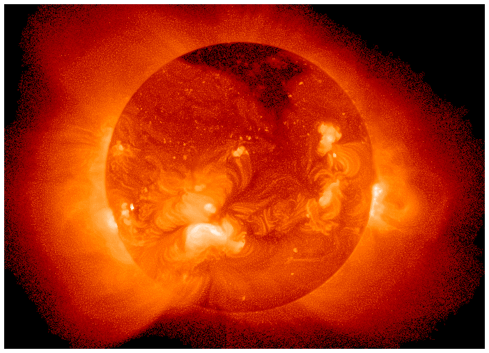
Figure 7A large coronal hole (the dark region) near the north pole of the Sun. The figure was taken by the soft X-ray telescope (SXT) onboard the Yohkoh satellite in 1992.
Figure 8 gives a “dial plot” of the solar wind speed for the first traversal of the Ulysses spacecraft over the Sun's poles. The radius from the center of the Sun to the trace indicates the solar wind speed. The magnetic field polarity is indicated by the color of the trace, red for outward IMFs and blue for inward IMFs. A SOHO EIT soft X-ray image of the Sun is placed at the center of the figure and a High Altitude Observatory Mauna Loa coronagraph image shows the inner corona at that time. The outer corona is an image taken by the SOHO C2 coronagraph.
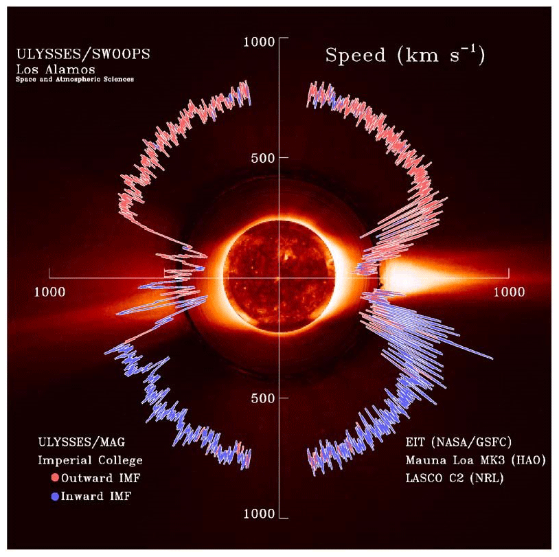
Figure 8High-speed solar wind streams emanating from coronal holes in the north and south solar poles. The figure was taken from Phillips et al. (1995) and Tsurutani (2006b).
Two large polar coronal holes are detected at the Sun, one at the north pole and the other at the south pole. It is noted that HSSs of ∼750 to 800 km s−1 are detected at Ulysses when over the polar coronal hole regions. When Ulysses was near the solar equatorial region where helmet streamers are present, the solar wind speeds are of the slow solar wind variety, Vsw∼400 km s−1. The reader should note that it took years for Ulysses to make this polar orbit, while the solar and coronal images were taken at one point in time. However, this composite figure is useful to illustrate the main points about the origins of HSSs.
3.2.2 High-speed solar wind streams and the formation of CIRs
Figure 9 shows a HSS–slow speed stream interaction during January 1974. The right portion of the top panel on day 26 shows a HSS with speeds of 750–800 km s−1 at 1 AU. On day 24, the top panel left indicates a solar wind speed of ∼300 km s−1, or the slow solar wind. The effects of the stream–stream interaction occur on day 25. This is best seen in the IMF magnitude panel, seventh from the top. The stream–stream interaction creates intense magnetic fields of ∼25 nT. The sixth from top panel is the IMF Bz component (in GSM coordinates). The Bz is highly fluctuating. Magnetic reconnection between the IMF southward components and the magnetopause magnetic fields leads to the irregularly shaped storm main phase shown in the bottom (Dst) panel.
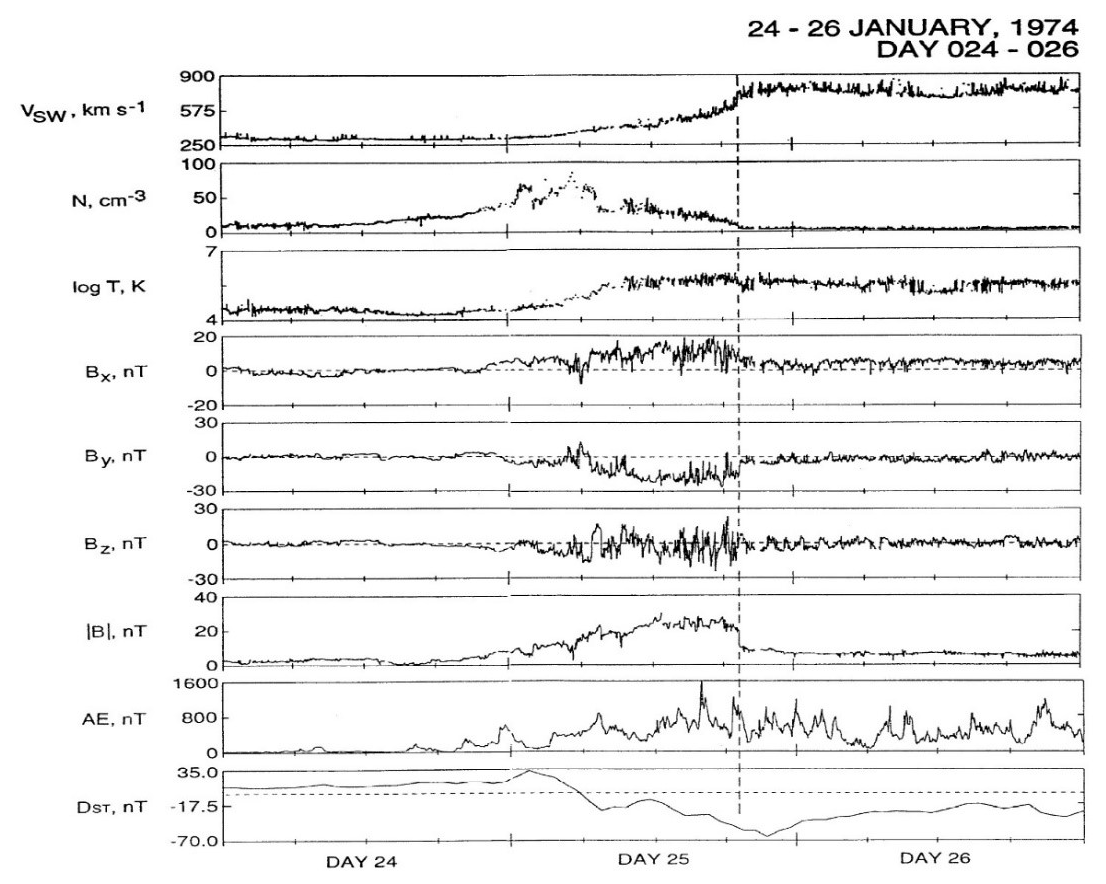
Figure 9A high-speed solar wind stream–slow solar wind interaction and the formation of a CIR during January 1974. The format is the same as in Fig. 4 except that the AE index is given in the next to bottom panel. The figure is taken from Tsurutani et al. (2006b).
To be able to forecast a CIR magnetic storm, one would have to first understand the sources of the IMF Bz fields. For example, are they compressed upstream Alfvén waves (Tsurutani et al., 1995, 2006c)? Or could they be waves generated by the shock interaction with upstream waves in the slow solar wind? That would be only the first step for forecasting, of course. Then with knowledge of the properties of the slow speed stream, the details of the wave compression/interaction would then have to be calculated/modeled.
Another approach would be to determine whether there is an underlying southward component of the IMF within the CIR. This would most likely be caused by the geometry of the HSS–slow speed stream interaction and may be predictable from MHD modeling. If this is correct, then the sheath fields can be modelled by a slowly varying field with highly fluctuating fields superposed on top of it. In (rare) cases of radial alignment, Solar Probe closest to the Sun could characterize sheath fields. The evolution of those fields would be detected by Solar Orbiter. Simulation of further evolution could be applied and predictions of the fields at 1 AU could be tested by ACE data. If there are waves generated by the shock, then the above scenario would not work as well as expected, or at least would be more complicated to apply in a useful manner.
3.2.3 High-speed solar wind streams, Alfvén waves and HILDCAAs
The schematic in Fig. 6 showed a long “recovery phase” that trails the CIR magnetic storm main phase (see Tsurutani and Gonzalez, 1987). However, we now know that the storm was not “recovering” as in the case of an MC magnetic storm recovery but that something else was occurring. This “recovery” can last from days to weeks. Thus, processes of charge exchange, Coulomb collisions, etc., for ring current particle losses are not tenable to explain such long “recoveries”.
Figure 10 shows the interplanetary cause of this extended geomagnetic activity. It occurs primarily during HSSs independent of whether a CIR magnetic storm occurred prior to it or not (Tsurutani and Gonzalez, 1987; Tsurutani et al., 1995, 2006b; Kozyra et al., 2006b; Turner et al., 2006; Hajra et al., 2013, 2014a, b, c, 2017). From top to bottom are the solar wind speed, the IMF magnitude, the IMF Bz component (in GSM coordinates) and the auroral electrojet (AE) index. The bottom panel is the Dst index.
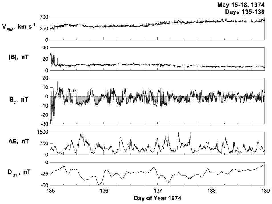
Figure 10A high-intensity, long-duration continuous AE activity (HILDCAA) event during 1974. Taken from Tsurutani et al. (2006c).
The interplanetary data were taken from the IMP-8 spacecraft, an Earth-orbiting satellite that was located upstream of the magnetosphere in the solar wind at this time. The location was inside 40 Re, where an Re is an Earth radius. The magnetic Bz fluctuations have been shown to be Alfvén waves which are of large nonlinear amplitudes in HSSs (Belcher and Davis, 1971; Tsurutani and Gonzalez, 1987; Tsurutani et al., 2018b). What is apparent from this figure is that every time the IMF Bz is negative (southward), there is an AE increase and a Dst decrease. This has been interpreted as being due to magnetic reconnection between the southward components of the Alfvén waves and the Earth's magnetopause. The AE is enhanced by the same magnetic reconnection process that occurs during substorms, and a small parcel of plasma-sheet plasma is injected into the nightside magnetosphere, causing the Dst index to decrease slightly. It is noted that there are many southward IMF Bz dips in this 4-day interval of data shown in Fig. 10. There are also many corresponding AE increases and Dst decreases. Thus, the interpretation of the constant/average Dst value of nT for 4 days is that continuous plasma injection and decay are occurring. This is clearly not a “recovery phase” where the ring current particles are simply lost; it only appears as a recovery from the Dst trace. Soraas et al. (2004) have shown that particles are injected during these events, but only to L values of 4 and greater (the L=4 magnetic field line is the dipole magnetic field that crosses the magnetic equator a distance of 4 Earth radii from the center of the Earth). These are shallow injections, as suggested above.
These geomagnetic activity events have been named high-intensity, long-duration continuous AE events or HILDCAAs (Tsurutani and Gonzalez, 1987). This name is simply a description of the events without an interpretation. In 2004 when a detailed examination using polar EUV auroral imaging was applied, it was found that many phenomena besides simple isolated substorms occurred (Guarnieri, 2006; Guarnieri et al., 2006). Although substorms occur during HILDCAA events, there are AE increases (injection events?) that are not well correlated with substorm onsets (Tsurutani et al., 2004b). The full extent of HILCAAs is not well understood (see also Souza et al., 2016; Marques de Souza et al., 2018; Mendes et al., 2017). By using IMAGE auroral observations and geomagnetic indices to identify convection events which are not classical Akasofu (1964) substorms, the fields and particle data from SWARM, MMS and Arase could be used to characterize the physics properties of these “convection” events.
There is also the question of the origin of the interplanetary Alfvén waves. Do they originate at the Sun caused by supergranular circulation or is that mechanism untenable, as argued by Hollweg (2006)? Could the waves be generated locally between the Sun and Earth, as speculated by Matteini et al. (2006, 2007) and Hellinger and Travnicek (2008)? Parker Solar Probe could identify Alfvén waves within high-speed streams and Solar Orbiter (when radially aligned) could determine the wave evolution.
The original requirement for identifying a HILCAA event was quite strict. The event had to occur outside of a magnetic storm main phase (Dst was required to be >−50 nT: Gonzalez et al., 1994), the peak AE intensity had to be greater than 1000 nT (high-intensity), the event had to last longer than 2 d (long-duration), and there could not be any dips in AE less than 200 nT for longer than 2 h (continuous). Clearly there are events with the same interplanetary causes and geomagnetic effects as for the strict definition. However, the strict definition is useful for further studies using different data sets.
3.2.4 HILDCAAs and the acceleration of relativistic magnetospheric electrons
One of the consequences of HSSs and HILDCAAs is the acceleration of relativistic (∼ MeV) electrons. These energetic particles can damage orbiting satellite electronic components (Wrenn, 1995) and thus are known as “killer electrons”. Figure 11 shows the relationship between the onset of HILCAA events (vertical line) and relativistic electron fluxes. From top to bottom are the E>0.6 MeV, the E>2.0 MeV and the E>4.0 MeV electron fluxes detected by the GOES-8 and GOES-12 satellites located at L=6.6. This figure is a superposed epoch analysis (Chree, 1913), the result of 35 HILDCAA events in solar cycle 23, from 1995 to 2008, which are not preceded by magnetic storms. The exclusion of magnetic storms was done to avoid contamination by storm-time particle acceleration (by intense convection/compression). The zero-epoch time (vertical line) corresponds to the HILDCAA onset time. Here the “strict” definition of HILDCAAs was used to define the onset times.
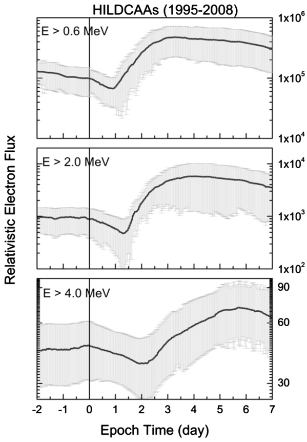
Figure 11The relationship between HILDCAAs and relativistic electron acceleration. The figure is taken from Hajra et al. (2015a).
The figure shows that the flux enhancement of E>0.6 MeV electrons is statistically delayed by ∼1.0 d from the onset of the HILDCAAs. The E>4.0 MeV electrons are statistically delayed by ∼2.0 d from the HILDCAA onset. It is thus possible that HILCAAs may be used to forecast relativistic electron flux enhancements in the magnetosphere (see Hajra et al., 2015b; Tsurutani et al., 2016a; Hajra and Tsurutani, 2018a; Guarnieri et al., 2018). This however has not been done yet and could be implemented by scientists today.
The physics for electron acceleration to relativistic (∼ MeV) energies has been well developed by magnetospheric scientists. Two competing acceleration mechanisms have been developed. In one mechanism, with each injection of plasma-sheet particles on the nightside magnetosphere, the anisotropic ∼10 to 100 keV electrons generate electromagnetic whistler mode chorus waves (Tsurutani and Smith, 1974; Meredith et al., 2002) by the loss cone/temperature anisotropy instability (Brice, 1964; Kennel and Petschek, 1966; Tsurutani et al., 1979; Tsurutani and Lakhina, 1997). The chorus then interacts with the ∼100 keV injected electrons to energize them to ∼0.6 MeV energies (Inan et al., 1978; Horne and Thorne, 1998; Thorne et al., 2005, 2013; Summers et al., 2007; Tsurutani et al., 2010; Reeves et al., 2013; Boyd et al., 2014). The lower-frequency part of the chorus in turn interacts with the ∼0.6 MeV electrons to accelerate them to ∼2.0 MeV energies. This bootstrapping mechanism has been suggested by several authors (Baker et al., 1979, 1998; Li et al., 2005; Turner and Li, 2008; Boyd et al., 2014, 2016; Reeves et al., 2016) and has been confirmed by Hajra et al. (2015a) during HILDCAA events.
An alternative scenario is that relativistic electrons are created through particle radial diffusion driven by micropulsations (Elkington et al., 1999, 2003; Hudson et al., 1999; Li et al., 2001; O'Brien et al., 2001; Mann et al., 2004; Miyoshi et al., 2004). However, the same general scenario would hold as for chorus acceleration. The substorms and convection events within HILDCAAs would be the sources of the micropulsations and the micropulsations would last from days to weeks in duration. Bootstrapping of energy would still take place.
An important question for researchers to ask is “How high can the relativistic magnetospheric electron energy get?”. If there are two HSSs, one from the South Pole and another from the North Pole so that Earth's magnetosphere is bathed in HSSs for years, as happened during 1973–1975 (Sheeley et al., 1976, 1977; Gosling et al., 1976; Tsurutani et al., 1995), will the energies go above ∼10 MeV? What will physically limit the energy range? This answer is important for keeping Earth-orbiting satellites safe during such events.
3.2.5 Solar wind ram pressure pulses and the loss of relativistic electrons
Figure 12 shows a relativistic electron decrease (RED) event occurring during 1998. From top to bottom are the E>0.6 MeV electron fluxes, the E>2.0 MeV electron fluxes, the solar wind speed, density and ram pressure, and the IMF magnitude and Bx, By and Bz components in the GSM coordinate system. The bottom two panels are the 1 min SYM-H index (a high time resolution Dst index) and the AE index. The relativistic electron measurements were taken at L=6.6.
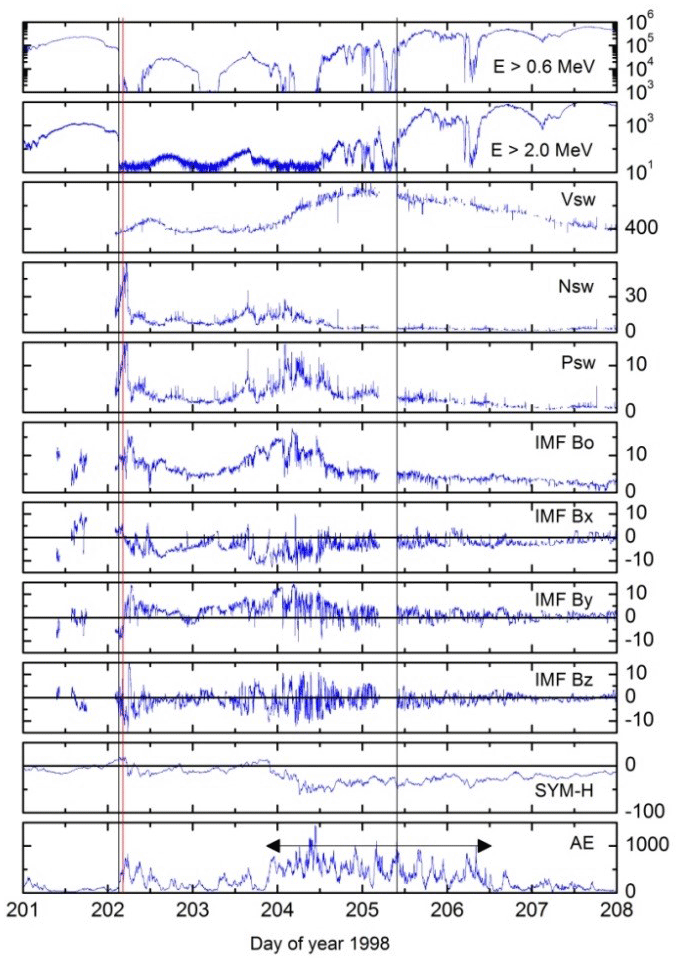
Figure 12A relativistic electron decrease (RED) event and later acceleration. Taken from Tsurutani et al. (2016b).
At the beginning of day 202, a vertical black line indicates the onset of a high-density HPS crossing (Winterhalter et al., 1994) that is identified in the fourth panel from the top. The HPS is by definition located adjacent to the HCS (Smith et al., 1978). The HCS is noted by the reversal in the signs of the IMF Bx and By components (seventh and eighth panels from the top). The onset of the HPS is followed within 1 h by the vertical red line, the sudden disappearance of the E>0.6 MeV (first panel) and E>2.0 MeV (second panel) relativistic electron fluxes. Tsurutani et al. (2016b) have shown that for eight relativistic electron flux disappearance events during solar cycle 23 all of the disappearances were associated with HPS impingements onto the magnetosphere.
Where have the relativistic electrons gone? There are two primary possibilities. One is that the energetic electrons have gradient drifted out of the magnetosphere through the dayside magnetopause, a feature that has been called “magnetopause shadowing” by West et al. (1972). However, a second possible mechanism is electron pitch angle scattering by electromagnetic ion cyclotron (EMIC) waves. We think that this second possibility is more intriguing and has far more interesting consequences, if correct. One might ask where the EMIC waves come from and why pitch angle scattering is particularly important. It has been shown by Remya et al. (2015) that when the magnetosphere is compressed, both electromagnetic chorus (electron) waves (Thorne et al., 1974; Tsurutani and Smith, 1974; Meredith et al., 2002) and EMIC (ion) waves (Cornwall, 1965; Kennel and Petschek, 1966; Olsen and Lee, 1983; Anderson and Hamilton, 1993; Engebretson et al., 2002; Halford et al., 2010; Usanova, 2012; Saikin, 2016) are generated. The compression of the magnetosphere causes betatron acceleration of remnant ∼10 to 100 keV electrons and protons, and thus plasma instabilities associated with both particle populations occur. What is particularly important is that the EMIC waves are coherent (Remya et al., 2015), leading to extremely rapid pitch angle scattering of ∼1 MeV electrons by the waves. The scattering rate has been shown to be 3 orders of magnitude faster than that with incoherent waves (Tsurutani et al., 2016b).
Another possible loss mechanism is associated with possible generation of PC waves by the HPS impingement followed by radial diffusion of the relativistic electrons. Wygant et al. (1998) and Halford et al. (2015) have mentioned that larger loss cone sizes at lower L could be a source of loss to the ionosphere. Rae et al. (2018) have shown that superposition of compressional PC waves and the conservation of the first two adiabatic invariants could enhance particle losses. However, one should mention that there are no observations of PC wave generation during HPS impingements, and this needs to be tested. It is also uncertain how rapidly the relativistic electrons would be lost by the above processes. It has been shown that the total loss of L>6.6 relativistic electrons occurs in ∼1 h (Tsurutani et al., 2016b).
Why can the loss of relativistic electrons to the atmosphere be important? Figure 13 shows the results of the GEometry ANd Tracking 4 (GEANT4) code developed by the European Organization for Nuclear Research (Agostinelli et al., 2003) applied to the relativistic electron disappearance problem. The GEANT4 code takes into account Rayleigh scattering, Compton scattering, photon absorption, γ-ray pair production, multiple scattering, ionization, bremsstrahlung for electrons and positrons and annihilation of positrons (positron formation is not germane for these “low energy” relativistic particles, but the code includes it anyway). A standard atmosphere was used.
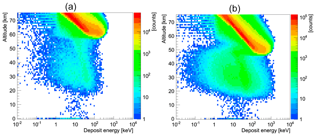
Figure 13The GEANT4 code run results for the precipitation of E>0.6 MeV electrons (left panel) and E>2.0 MeV electrons (right panel). The vertical scale is altitude above the ground and the horizontal scale is energy deposition. The color scheme (legend on the right) gives the number of counts. Taken from Tsurutani et al. (2016b).
Figure 13 shows the GEANT4 Monte Carlo results for the electron shower for E>0.6 MeV electrons on the left and for E>2.0 MeV electrons on the right. Two important features should be noted. First the bulk of energy deposition (the red areas) descends to ∼60 km for the E>0.6 MeV electron simulation and to ∼50 km for the E>2.0 MeV electron simulation. This portion of the energy from the incident electrons is due to direct ionization and particle energy cascading. However, there is a second region which might be extremely important, that is, the blue-green area that goes down to ∼20 km for the E>0.6 MeV simulation and ∼16 km for the E>2.0 MeV simulation. There are also “hits” seen on the ground. This lower-altitude energy deposition is due to the relativistic electrons interacting with atmospheric atomic and molecular nuclei creating bremsstrahlung X-rays and γ-rays. X-rays and γ-rays have very large mean free paths and thus can freely propagate through the dense atmosphere without interactions. They propagate to much lower altitudes where they interact and continue the energy cascading process further.
The reason why this process may be quite an important space weather topic is that it might relate to atmospheric weather as well. Wilcox et al. (1973) discovered a correlation between interplanetary HCS crossings and high-atmospheric vorticity winds at 300 mb altitude. Over the years a number of different explanations for the physics of the trigger have been offered (Tinsley and Deen, 1991; Lam et al., 2013). Tsurutani et al. (2016b) presented the above relativistic electron precipitation scenario (instead of HCS crossings) for the possible triggers of high-atmospheric vorticity winds. Quantitative estimates of potential energy deposition at different atmospheric altitudes were provided in the original paper.
It is noted that the energy deposition should occur in a limited spatial region of the globe (just inside the auroral zone and a small region of the dayside atmosphere), which is more geoeffective than either cosmic ray energy or solar flare particle deposition. The fact that it is relativistic electron precipitation gives an additional advantage that substantial energy is deposited at quite low altitudes.
Advances to this problem can be made in a number of different ways. Simultaneous ground-detected EMIC waves, γ-rays and atmospheric heating/cooling could be sought. Correlation with such events with solar wind pressure pulses like the HPSs or interplanetary shocks (see Hajra and Tsurutani, 2018b) would advance our knowledge of the details of such events.
Maliniemi, Asikainen and Mursula (2014) studied the Earth's winter surface temperatures and the North Atlantic Oscillation (NAO) during all 4 phases of the solar cycle using 13 solar cycles of data (1869–2009). The authors found that the clearest pattern for temperature anomalies is not during sunspot maximum or minimum but during the declining phase when the temperature pattern closely resembles that found during positive NAO. This feature could be due to the energetic 10–100 keV electron precipitation discussed earlier.
Atmospheric heating events known as sudden stratospheric warmings (SSWs) (Scherhag, 1960; Harada et al., 2010) occur at subauroral latitudes by unknown causes. They are known to be related to atmospheric wind system changes, perhaps the same phenomenon as the Wilcox et al. (1973) effect. Atmospheric scientists generally assume that SSWs are created by gravity waves propagating from the lower atmosphere upward, but so far no one-to-one correlated case has been found. Thus, it would be quite interesting to see whether space weather can have a major impact on atmospheric weather. The connection between these two disciplines could be quite interesting for the next generation of space weather scientists.
3.2.6 Energetic particle precipitation and ozone depletion
Figure 14 shows two solar cycles of data, SC22 and SC23. From top to bottom are the “importance” of high-speed streams, the descending NOx, the monthly AA index, and the percent auroral power due to three types of solar wind phenomena (ICMEs, HSSs and slow solar wind), and the bottom panel solid line trace is the sunspot number (SSN). Also shown in the bottom panel is the solar energetic particle (SEP) flux.
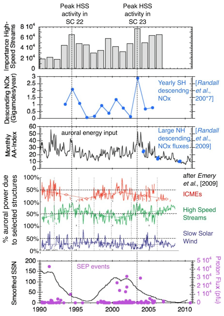
Figure 14The dashed vertical lines show the peaks in solar wind high-speed streams during SC 22 and SC 23. These are coincident with the peaks in auroral energy input and the peaks in yearly NOx descent. The authors thank Janet Kozyra for providing this unpublished figure.
There are two vertical dashed lines. They correspond to the peaks in HSS activity for SC22 and SC23 (top panel), peaks in auroral energy input (third panel from the top), and peaks in the yearly descending NOx (second panel from the top). It is noted that all three peaks are aligned in time. The bottom panel shows that both dashed vertical lines correspond to times in the descending phase of the solar cycle.
Figure 15 shows the Kozyra et al. (2019) scenario for ozone destruction over the polar cap. The top of the figure shows the various types of solar wind (and associated energetic particles) that can affect atmospheric ozone. The quiet solar wind will lead to quiescence. HSSs lasting a few to 10 days have weak effects, and ICMEs (and of course shock acceleration of energy particles) can have much stronger effects.
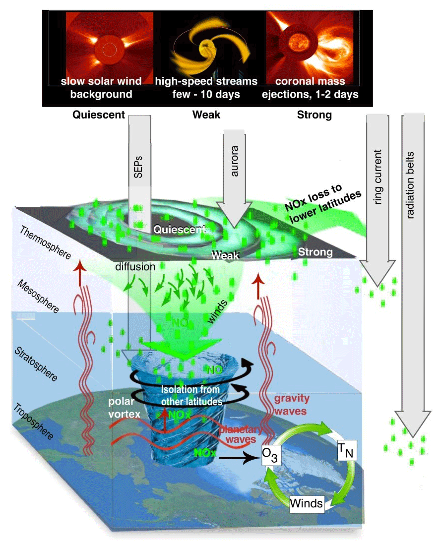
Figure 15The scenario for polar cap ozone destruction using the observations shown in Fig. 14. The authors thank Janet Kozyra and her colleagues (personal communication, 2019) for this unpublished figure.
Energetic particles from different sources will precipitate in different regions of the ionosphere. The energetic particles associated with interplanetary CME shock acceleration will be deposited in the polar regions of both the northern and southern ionospheres. If the particles are energetic enough with sufficient gyroradii, they can reach latitudes as low as ∼50∘ magnetic latitude. Precipitating substorm/HILDCAA ∼10–100 keV magnetospheric charged particles will deposit their energy on closed auroral zone (∼60 to 70∘) magnetic field lines.
The energetic particles entering the atmosphere lose a portion of their energy in the dissociation of N2 into N+N. The nitrogen atoms will attach to oxygen atoms to form NOx. Auroral HILDCAA ∼10–100 kev energy particles will only penetrate to depths of ∼75 km above the surface of the Earth. Solar energetic particles with greater kinetic energies can penetrate lower into the atmosphere to ∼50 to 60 km. If there is a polar vortex, this vortex can “entrain” the NOx molecules and atmospheric diffusion can bring them down to lower altitudes over months in time duration. The NOx can act as a catalyst in the destruction of ozone.
One interesting consequence of extreme ICME shocks is that one would expect extreme Mach numbers to lead to both extreme SEP fluences and also extremely high energies. The former will lead to greater production of NOx int the polar regions and the latter to deeper penetration and thus less loss of NOx as they diffuse downward. Alternatively there is a scenario where radiation belt “killer” relativistic electrons can play an important role. If there are large solar polar coronal holes like in 1973–1975, HSSs could produce extremely intense and energetic relativistic electrons. Shocks and HPS impingements on the magnetosphere could cause loss of the electrons to the lower atmosphere. This magnetospheric energy pumping and dumping may have important consequences for NOx production. The topic of shock acceleration of energetic particles will be discussed in more detail in Sect. 4.1.
4.1 Interplanetary shocks and energetic charged particle acceleration
Interplanetary shocks have a variety of effects on both interplanetary space and the Earth's magnetosphere. It is important for the reader to note that these space weather phenomena can occur with or without the occurrence of magnetic storms. Shock and magnetic storm intensities are related, but only in a loose sense. The physical mechanisms for energy transfer for different phenomena are different. As one example, interplanetary shock acceleration of energetic charged particles (called “solar cosmic rays”) is due to an ICME ram energy driving the fast shocks, which then transfers energy to the charged particles. Solar cosmic ray events can occur with or without magnetic storms (Halford et al., 2015, 2016; Mays et al., 2015; Foster et al., 2015). Some of the major extreme space weather topics will be addressed below.
Acceleration of energetic particles in deep space was discovered by Pioneer 11 energetic particle scientists (McDonald et al., 1976; Barnes and Simpson, 1976; Pesses et al., 1978, 1979; Van Hollebeke et al., 1978; Christon and Simpson, 1979). As the Pioneer 11 spacecraft traveled away from the Sun, it was found that the particle fluences kept increasing, contrary to the concept of adiabatic deceleration. The interplanetary magnetic field magnitude decreases with increasing distance from the Sun, so one would expect energetic particle deceleration with distance. Thus it was clear to scientists that something must be accelerating these particles in the interplanetary medium. Figure 16 shows one channel of the Pioneer 11 energetic proton count rate, ∼0.5 to 1.8 MeV (see Simpson et al., 1974). The bottom panel is the Pioneer 11 magnetic field (Smith et al., 1975). Some of the peak magnetic fields are numbered, corresponding to a ∼25 d recurrence of these magnetic structures. The magnetic magnitude structures are identified as well-developed CIRs (see Smith and Wolfe, 1976), bounded by fast forward and fast reverse shocks.
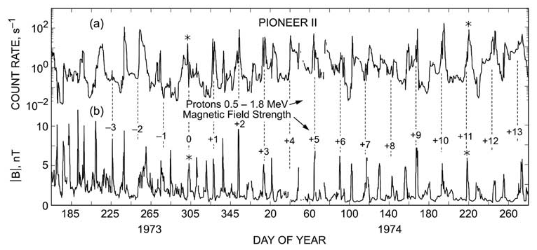
Figure 16Energetic ∼0.5 to 1.8 MeV protons accelerated by interplanetary fast forward and fast reverse shocks. Taken from Tsurutani et al. (1982).
Tsurutani et al. (1982) identified the shocks and showed statistically that both forward and reverse shocks were related to proton peak count rates. One of the results, which still remains to be solved, is that the proton peaks were generally higher at the reverse shocks. What is the mechanism for greater particle acceleration at fast reverse shocks? This has received little attention and should be addressed in the future.
Reames (1999) has argued that fast forward shocks upstream (anti-solarward) of ICMEs are the most important phenomenon for the acceleration of “solar flare” particle events. Particle acceleration occurs throughout interplanetary space from near the Sun (where the shocks first form) to 1 AU and beyond as the shocks propagate through the heliosphere. Studies of this acceleration as a function of longitudinal distance away from magnetic connection to the flare site (this gives the variations in the shock normal angle and thus dominant mechanism for acceleration – see Lee, 2017, and references therein) have been done by Lario (2012). The features of the energetic particles in space have different characteristics depending on these distances and the portion and characteristics of the shock that the particles are being accelerated from.
Forecasting the solar flare/interplanetary shock features such as the fluence, energy, spectra and composition will require knowledge of the upstream seed population, upstream (and downstream) waves, and shock properties such as the magnetosonic Mach number and shock normal angle. This is a very difficult task since knowledge of the entire slow solar wind plasma from the Sun to 1 AU will be required for accurate forecasting. But again, the Parker Solar Probe and Solar Orbiter may help in developing two points of measurements for modeling of specific events.
A more fundamental problem is why measured interplanetary fast forward shock Mach numbers at 1 AU are so low. As previously mentioned, Tsurutani and Lin (1985) from ISEE-3 measurements have found that at 1 AU, the measured magnetosonic Mach numbers were typically only 1 to 3. Tsurutani et al. (2014) have identified a shock with Mach number ∼9 and Riley et al. (2016) have identified an event with magnetosonic Mach number ∼28. The latter event was associated with the SOHO 2012 extreme ICME which did not impact the Earth's magnetosphere. The above are extreme events and few or no events have been detected with intermediate values. A study is needed to determine shock Mach numbers at different distances from the Sun. These will give clues as to why 1 AU shock Mach numbers are so low. Is the acceleration of energetic particles causing the dissipation of shock energy as they propagate from the Sun to 1 AU? Data from Parker Solar Probe, Solar Orbiter and ACE could be useful in this regard.
In a related issue, the use of STEREO imaging and MHD modeling could be useful to determine the mass loading of ICME sheaths in causing the deceleration of the ICMEs. This deceleration will also lower the Mach number of the shocks.
4.2 Extreme interplanetary shocks and extreme interplanetary energetic particle acceleration
Tsurutani and Lakhina (2014) have shown from simple calculations that for CMEs with extreme speeds of 3000 km s−1 (Yashiro et al., 2004; Gopalswamy, 2011), shock Mach numbers of ∼45 are possible. These Mach numbers get close to expected supernova shock values. Why have such strong shocks not been observed at 1 AU? If such events are possible, what would the energetic particle fluences be? Experts on shock particle acceleration will hopefully answer this complex question. It is well known that such solar flare particles enter the polar regions of the Earth's atmosphere and cause radio blackouts. Will extreme solar flare particle fluence precipitation cause different ionospheric effects other than those known today? This latter question might be addressed by ionospheric modelers.
It should be noted that although space weather is a chain of events/phenomena going from the Sun to interplanetary space to the magnetosphere, ionosphere and atmosphere, there is often no direct link between different facets of space weather. Each feature of space weather should be examined separately, and it should not be assumed that an extreme flare will cause extreme cascading space weather phenomena. We use solar flare particles as an example for the reader. The largest solar flare particle event in the space age occurred in August 1972 (Dryer et al., 1976, and references therein). However, there was no magnetic storm caused by the MC impact on the Earth's magnetosphere (the MC field was directed almost entirely northward, leading to geomagnetic quiet: Tsurutani et al., 1992b). On the other hand, the largest magnetic storm on record is the Carrington storm. The storm intensity will be discussed further in Sect. 7. There is little or no evidence of large solar flare particle fluences in Greenland ice-core data from that event (Wolff et al., 2012; Schrijver et al., 2012). Usoskin and Kovfaltsov (2012), examining historical proxy data (14C and 10Be), also find a lack of any signature associated with the Carrington flare. Although this is an extreme example, it is useful to mention it to illustrate the point: different facets of space weather may have only loose correlations with other facets.
An area that has received a lot of attention lately is ancient solar flares. Miyake et al. (2012) discovered an anomalous 12 % rapid increase in 14C content from AD 774 to 775 in Japanese cedar tree rings. Usoskin et al. (2013) have argued that such an extreme radiation event could be associated with an extreme solar energetic particle event (or a sequence of events). The latter authors estimated that the fluence of >30 MeV particles was cm−2. Could such an extreme particle event be associated with an extremely strong interplanetary shock or instead series of strong shocks? Space weather scientists are currently working on this problem.
4.3 Interplanetary shocks, dayside aurora and nightside substorms
Interplanetary shocks can trigger the precipitation of energetic ∼10 to 100 keV electrons into the auroral ionosphere (Halford et al., 2015). In fact, low-energy (E<10 keV) electron precipitation can occur as well. Figure 17 shows interplanetary shock impingement auroral UV effects for an event on 23 September 1998. Each image has the north pole at the center and 60∘ MLAT shown at the outer edge. Noon is at the top and dawn is at the right. The cadence between images is ∼1 min 13 s. From ACE measurements and propagation calculations it is known that the fast forward shock arrived the magnetosphere between images (c), 23:44:44 UT and (d), 23:45:47 UT. What is apparent in panel (d) is the sudden appearance of an aurora on the dayside (Zhou and Tsurutani et al., 1999). From further analyses of these shock auroral events, Zhou et al. (2003) have shown that magnetospheric compression of preexisting ∼10 to 100 keV electrons and protons will generate both electromagnetic electron and proton plasma waves and diffuse auroras (as discussed previously). Also noted were the generation of field-aligned dayside currents. Compression of the magnetosphere will generate Alfvén waves (Haerendel, 1994) which will propagate along the magnetic field lines down to the ionosphere. Wave damping could provide substantial ionospheric heating.
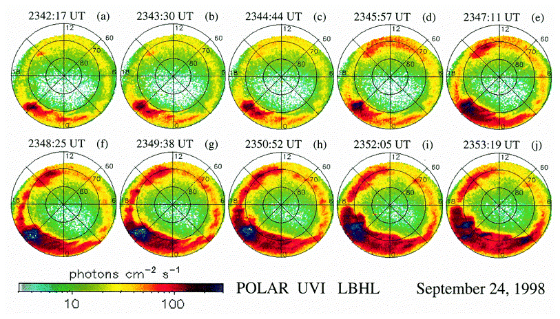
Figure 17Interplanetary shocks cause dayside auroras and trigger nightside substorms. The images show the northern polar views of polar cap and auroral zones taken at UV wavelengths. Local noon is at the top in each image. The figure is taken from Zhou and Tsurutani (2001).
The mechanism for energy transfer from the solar wind to the magnetosphere is the absorption of the solar wind ram energy. Dayside auroras occur with shock impingement irrespective of the interplanetary magnetic field Bz direction. Other possible mechanisms for the dayside aurora not mentioned above are double layers above the ionosphere (Carlson et al., 1998) with the acceleration of ∼1 to 10 keV electrons and the formation of discrete dayside auroras. What is the relative importance of these three different auroral energy mechanisms? This would be an excellent topic for the SWARM and Arase satellite missions. Coordinated ground measurements would be useful.
Returning to Fig. 17e 23:47:11 UT, there is a substorm intensification centered at ∼2100 magnetic local time (MLT). The substorm further intensification and expansion can be noted in the sequence of images. Interplanetary shock triggering of substorms has been known to occur before the advent of imaging polar-orbiting spacecraft (Heppner, 1955; Akasofu and Chao, 1980). The AE index had been used to identify these events.
Important fundamental questions for substorm physics that have existed for a long time are where in the tail/magnetosphere the substorm gets initiated and by what physical mechanism. Is it reconnection or plasma instabilities (Akasofu, 1972; Hones, 1979; Lui et al., 1991; Lui, 1996; Baker et al., 1996; Lakhina, 2000)? Where does the energy come from, recent precursor solar wind inputs as suggested by Zhou and Tsurutani (1999) or stored tail energy or even possibly solar wind ram energy (see Hajra and Tsurutani, 2018b)? The rapid response of the magnetosphere to the shock should limit the downstream location of the substorm initiation point. It should be noted that there are probably several different mechanisms for causing substorms. Although this is only the shock triggering case, knowledge of this may help understand other cases, if they are indeed different. The MMS mission will be ideally suited for addressing this question in the tail phase of the mission.
4.4 Interplanetary shocks and the formation of new radiation belts
Figure 18 shows evidence of a new “radiation belt” triggered by a strong interplanetary shock. The figure shows three traces, E>6, >9 and >13 MeV fluences. At the time of the strong and sudden increase in all energy fluxes, the spacecraft was at L=2.6. This is time-coincident with the shock impingement upon the magnetosphere (not shown). With increasing time, a second, then third, etc., electron flux pulse appears. These are “drift echoes” where the energetic electron “cloud” has gradient drifted around the magnetosphere to return to the satellite location once again.
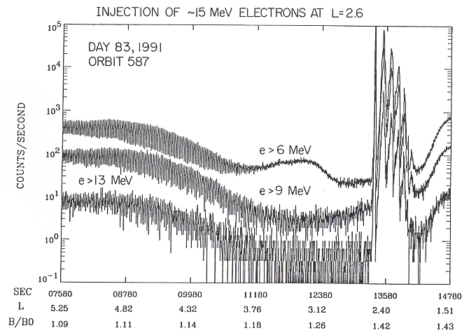
Figure 18Shock creation of a new relativistic electron radiation belt in the magnetosphere. The three energy channel plots show an abrupt increase in flux at the same time. Recurrence of the flux with decreasing amplitude occurs at least four more times. Figure taken from Blake et al. (1992).
4.4.1 What is the mechanism to create this new radiation belt?
Figure 19a shows an expanded version of Fig. 16 on the top with the addition of the ∼10 to 50 MeV count rate channel included. Next is the direct current electric field in the Y direction and magnetospheric Bz at the bottom. Panel (b), bottom, shows a magnetic pulse input into the system. This generates a time-varying azimuthal electric field (right middle) and the relativistic electron flux at the top right.
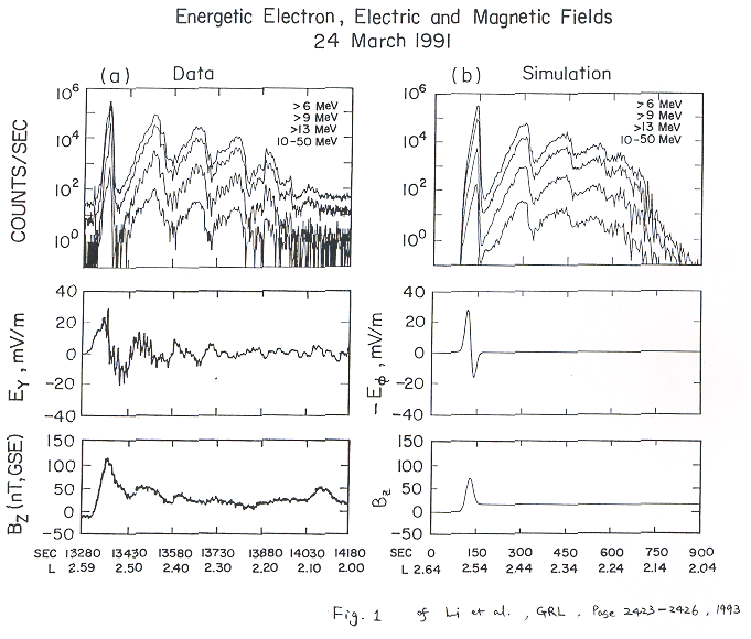
Figure 19An expanded version of the relativistic electron pulse and measured magnetospheric electric field and magnetic field Bz on the left and simulation results on the right. Taken from Li et al. (1993).
Using the input of a single magnetospheric magnetic pulse into the magnetosphere, Li et al. (1993) simulated the acceleration and injection of E>40 MeV electrons. What is interesting is that the origin of the electrons was L>6 with energies of only a few MeV. The reader should read Li et al. (1993) for more details concerning the simulation and results. Related works on acceleration of magnetospheric electrons by shock impact on the magnetosphere can be found in Wygant et al. (1994), Kellerman and Shprits (2012), Kellerman et al. (2014), and Foster et al. (2015).
How strong was the interplanetary shock? There was no spacecraft upstream of the Earth at the time of the event, so no measurements of shock strength can be made. However, Araki (2014) has noted that this shock caused a SI+ of magnitude 202 nT. This is the second largest SI+ in recorded history. In Tsurutani and Lakhina (2014) with the assumption of a 3000 km s−1 CME and only a 10 % deceleration from the Sun to 1 AU, they estimated a maximum SI+ of 234 nT under normal conditions. Could this 1991 shock strength have been close to the M=45 estimate mentioned earlier? One cannot really tell for sure because the shock Mach number strongly depends on the upstream plasma conditions, which can only be estimated in this case.
Tsurutani and Lakhina (2014) estimated a dB∕dt 6 times larger than the one used in the Li et al. (1993) modeling. What would a maximum dB∕dt cause in a new radiation belt formation? How much greater could the relativistic electron energy and flux become?
Figure 20 shows four well-known solar X-ray flare events taken in a narrow-band 26–34 nm EUV spectrum. The four flare events are the Bastille Day (14 July 2000) flare and three “Halloween” flares occurring on 28 and 29 October and 4 November 2003. The narrow-band EUV spectrum is shown because some of the flare X-ray and EUV fluxes were so intense that most spacecraft detectors became saturated (all except the SOHO SEM narrow-band EUV detector). The X-ray flare intensities could only be estimated from fitting techniques for the saturated data. Here we use the narrow-band channel of the SOHO SEM detector where the four abovementioned flares were not saturated. The four flare count rate profiles were aligned so that they start at time zero. What is particularly remarkable is that the 28 October 2003 flare has the highest EUV peak intensity of all four events and was greater by a factor of ∼2. This is the most intense EUV solar flare in recorded history.
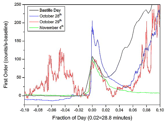
Figure 20The largest solar EUV flare in recorded history, 28 October 2003. Taken from Tsurutani et al. (2005b).
After each flare reached a peak intensity and then decreased in count rate, there was often a following increase in count rate. This is particularly notable in the Bastille Day (black trace) flare. This increase is contamination due to delayed energetic electrons propagating through space along interplanetary magnetic field lines reaching the spacecraft later in time. The 4 November flare (green) did not have such contamination because it was a limb flare, and presumably (magnetic) connection from the flare site to the spacecraft did not occur.
NOAA personnel have estimated that the November 4 flare had an intensity of ∼ X28. This event saturated the detector, so this is a conservative estimate. Thomson et al. (2004), using a different technique, estimated a value of X45 for this event. NOAA has estimated the 28 October flare to be ∼ X17. However, in EUV fluxes, the 28 October flare was the most intense by far.
Figure 21 shows the global total electron content (TEC) in the ionosphere after the 28 October 2003 solar flare. The map has been adjusted so Africa, the subsolar point, is in the center of the figure. The top and bottom of the plot correspond to the Earth's polar regions and the left-hand-side and right-hand-side edges to local midnight. The enhanced TEC area corresponds to the sunlit hemisphere. At the subsolar point the TEC enhancement was ∼30 %. This is the record for flare-induced ionospheric TEC (Tsurutani et al., 2005b). The nightside hemisphere shows no TEC enhancement, as expected. The TEC enhancement is due to ionization by X-rays, EUV photons and UV photons, all part of the solar flare spectrum.
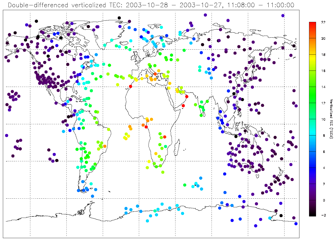
Figure 21The global TEC during the 28 October 2003 solar flare. The scale is given on the right. The figure is taken from Tsurutani et al. (2005b).
Figure 22 shows the effects of the 28 October solar flare. From top to bottom are the SOHO SEM EUV count rate, the GOES X-ray flux, the Libreville, Gabon, TEC data and the GUVI O and N2 dayglow data. It is noted that the flare profiles in EUV and X-rays last ∼ tens of minutes and are similar in profile to each other. However, the TEC over Libreville lasts hours. This is due to the EUV portion of the solar flare. These photons deposit their energy at ∼170 to 220 km altitude where the recombination timescales are ∼3 to 4 h. Thus, EUV photon ionization has longer lasting ionospheric TEC effects. The X-ray portion of the solar flare spectrum deposits its energy in the ∼80 to 100 km altitude range where the recombination timescale is tens of minutes (Thomson et al., 2005, and references therein). This solar flare example is one where solar energy (photons) goes directly from the Sun to the Earth's ionosphere (previously shown examples such as with ICMEs and sheaths with magnetic storms have solar plasma and magnetic field energy transfer from the Sun to interplanetary space to the magnetosphere).
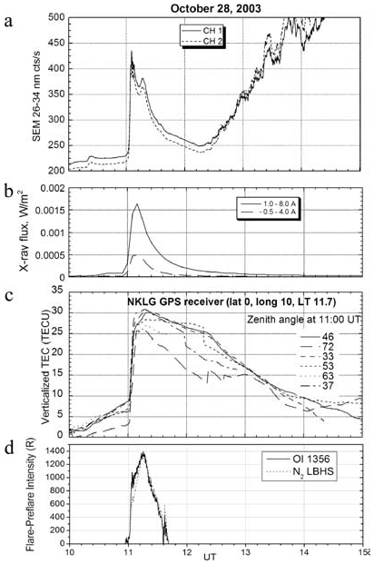
Figure 22The ionospheric and atmospheric effects of the 28 October 2003 solar flare. Taken from Tsurutani et al. (2005b).
Some future space weather problems are to be able to predict the solar flare energy spectrum given the underlying solar flare surrounding geometry. We have indicated that the 28 October 2003 and 4 November 2003 flares were significantly different spectra-wise. The question is why and how often does this happen? Ionospheric satellites like the Constellation Observing System for Meteorology, Ionosphere and Climate-2 (COSMIC II) and SWARM can probe for detailed altitude dependence of ionization to work backwards to attempt to identify which energy spectrum would cause the layered ionization detected. Solar flare data taken by instrumentation onboard the RHESSI and EVE/SDO spacecraft would be useful to understand the details of flare spectral differences. Other questions are how large can X-ray and EUV flares become? What will their ionospheric effects be?
For substorms, PPEFs occurring in the ionosphere have been known for a long time, since the beginning of the space age (Nishida and Jacobs, 1962; Obayashi, 1967; Nishida, 1968; Kelley et al., 1979, 2003). In the last 10 years lots of work has been done on PPEFs during magnetic storms. Why did people not look at storms earlier? Because it was theoretically predicted that the PPEFs would be shielded out. Why does shielding not happen? This is a very good question for workers in the field. Right now we do not know the answer.
Figure 23 shows the geometry of the Earth's magnetic field near the magnetic equator. It is parallel to the Earth's surface at the equator, but where the equatorial ionization anomalies (EIAs) are located, the magnetic field is slanted. The EIAs are standardly located at ∘ MLAT in the dayside ionosphere. With red arrows, the figure also shows the direction of E×B convection. At exactly the magnetic equator, E×B is in a purely upward direction. At the positions of the EIAs, the E×B direction is both upward and to higher absolute magnetic latitudes.

Figure 23Dayside (near)equatorial ionization anomalies (EIAs) located ∘ on both sides of the magnetic equator. The local Earth magnetic field is shown in this schematic. The figure is taken from Anderson et al. (1996).
Figure 24 shows three passes of the CHAMP satellite in polar orbit with an altitude of ∼430 km at the near-equatorial crossings. The three orbits are given in the upper right-hand side portion of the figure. The first TEC trace shown in blue is before the onset of the 30–31 October magnetic storm. The two EIAs are identified by the TEC enhancements at ∘ with peak intensities of ∼80 TEC units. In the next pass (red trace), the EIAs are located at ∘ MLAT and the peak intensities are ∼210 TEC units. During the next satellite pass, the EIAs are located near ±30∘ and the TEC values become as high as ∼330 TEC units. This “movement” of the EIAs to higher magnetic latitudes can be explained by a convective electric field (PPEF) in the east–west direction causing an uplift to both EIAs by E×B convection as explained earlier in connection with Fig. 23. One might ask why the TEC increases to such high values.
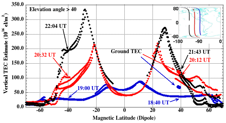
Figure 24Three passes of the CHAMP satellite measuring the near-equatorial and midlatitude TEC during 30 October 2003. CHAMP was at an altitude of ∼430 km, so the TEC measured was the total thermal electron column density above that altitude. The figure is taken from Mannucci et al. (2005).
The answer is that as the PPEF removes the plasma from the ionospheric lower F region and brings it to higher altitudes where the recombination timescale is longer (hours), the Sun's EUV photons replace the plasma by photoionization of the upper atmosphere, replacing the lost plasma and thus increasing the “total electron content” of the ionosphere. This is one cause of a “positive ionospheric storm”.
Figure 25 shows the interplanetary motional electric field for southward interplanetary Bz. The electric field will be in the dawn-to-dusk direction. When magnetic reconnection takes place in the nightside plasma sheet, the convective electric field will be in the same direction, but with a reduced amplitude. This electric field brings the plasma-sheet plasma into the nightside low-L region magnetosphere during magnetic storms. The PPEFs penetrate into the dayside equatorial ionosphere (shown in Fig. 24) and also the nightside equatorial ionosphere. However, significantly different from the dayside case, the E×B convection on the nightside will bring the ionospheric plasma to lower altitudes, leading to recombination and reduction in TEC. This is one form of a “negative ionospheric storm”. See Mannucci et al. (2005, 2008) for discussions of positive and negative ionospheric storms.
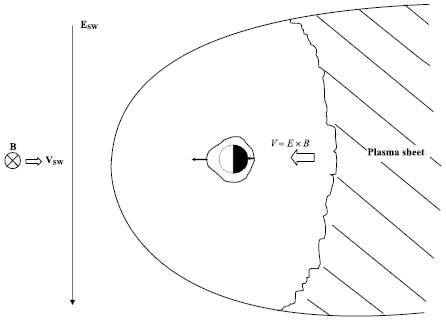
Figure 25The interplanetary, magnetospheric and equatorial ionospheric electric fields during a PPEF event. The figure is taken from Tsurutani et al. (2004c, 2008b).
There are many important questions about PPEFs which are almost always present during major magnetic storms. As previously mentioned, “why are the electric fields not shielded out?” What is the mechanism for generating PPEFs, wave propagation from the polar ionosphere as suggested by Kikuchi and Hashimoto (2016) or a more global picture as Fig. 25 and Nishida and Jacobs (1962) suggest? Figure 25 is a simple schematic. What are the real local time dependences of the PPEF? Does this vary from storm to storm, and if so, why? Why does the relative PPEF magnitude vary from one storm to the next? Again, future spacecraft and ground-based studies will be able to help answer these questions.
Figure 26 is the active region (AR) that was hand-drawn by Richard Carrington. This was the source of the optical solar flare that he and Hodgson (1859) saw and reported on 1 September 1859. See Cliver (2006) for a nice accounting of the observational activity taken during the 1859 flare interval and Kimball (1960) for an accounting of the aurora during the storm. The optical part of the flare lasted only ∼5 min. Some ∼17 h 40 min later a magnetic storm occurred at Earth (Carrington, 1859).
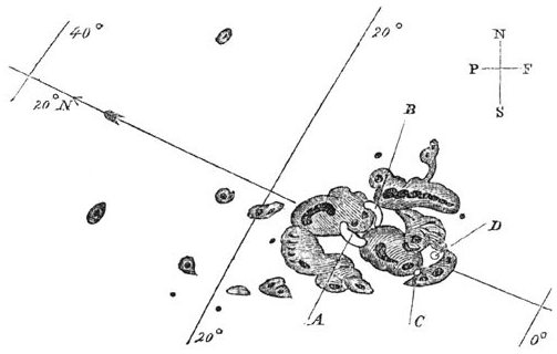
Figure 26The solar active region during the Carrington 1 September 1859 optical solar flare. The figure is taken from Carrington (1859).
Figure 27 shows the H-component magnetic field taken by the Colaba magnetic observatory during the Carrington magnetic storm. The SI+ is estimated to be ∼110 nT and the magnetic decrease ∼1600 nT at Colaba (Mumbai, India). The SI+ and storm main phase have been recently shown to be most likely caused by an upstream solar wind density of 5 particles cm−3 and a MC with intensity ∼90 nT (pointed totally southward) by Tsurutani et al. (2018a). No particularly unusual solar wind conditions are believed to have been necessary (in contrast to the original conclusions of Ngwira et al., 2014). Ngwira et al. (2018) is now in accord with this more recent assessment of a normal upstream solar wind.
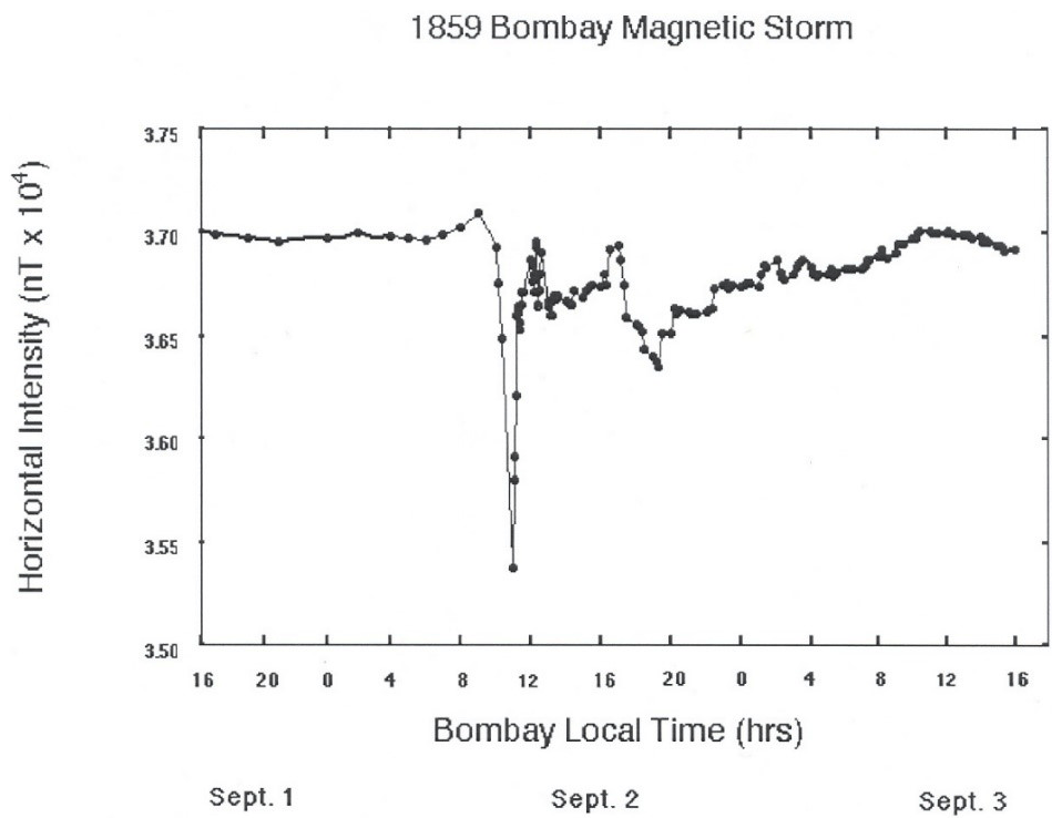
Figure 27The Carrington storm detected in the Colaba, India, magnetometer. The figure is taken from Tsurutani et al. (2003) and Lakhina et al. (2012).
The intensity of the Carrington storm was estimated as nT (Tsurutani et al., 2003) based on observations of the lowest latitude of red auroras being at ±23∘ (Kimball, 1960). The storm intensity was calculated using recent theoretical expressions of magnetospheric potentials needed to convect plasma into such low latitudes. Siscoe (1979), basing his estimate on a model that treats the pressure as a constant along the magnetic flux tube, came up with a value of nT.
It should be mentioned that some researchers have taken exception to the Colaba magnetogram as an indication of ring current effects (see the comment by Akasofu and Kamide (2005) and the reply by Tsurutani et al. (2005a)). The Colaba magnetic profile is unlike those of ICME magnetic storms discussed in Sects. 2.3, 2.4 and 3.1 of this paper. Several researchers have estimated the storm intensity based on the Colaba magnetogram (see the articles in a special journal edited by Clauer and Siscoe, 2006; Acero et al., 2018). The Colaba data clearly show that the storm had exceptionally large geomagnetic effects, regardless of the interpretation of the Colaba data. Possible interpretations of the Colaba profile will be discussed later in the paper.
The most accurate method of estimating a magnetic storm intensity is by using the latitude of the aurora. Red auroras (stable auroral red or SAR arcs) are presumably an indication of the location of the plasmapause (Richard M. Thorne, personal communication, 2002). Kimball (1960) noted that “red glows” were detected at ±23∘ from the geomagnetic equator during the Carrington event. In 1960 the term “SAR arc” was not in use, but we can assume that this was what he was reporting. At the present time, these are the most equatorward SAR arcs that have been observed (thus the most intense magnetic storm), that is, until researchers find records of even lower-latitude red auroras.
Comments on the short duration of the recovery phase have been made by Li et al. (2006). A high-density filament was used to explain this unusual feature of the magnetic storm profile. Tsurutani et al. (2018a) have recently proposed another possibility. During extreme events when the storm-time convection brings the plasma sheet into very low L, all of the standard ring current loss process rates will be enhanced. There will be greater Coulomb scattering, greater charge exchange loss rates and greater plasma wave growth with consequential greater wave–particle pitch angle scattering and losses to the atmosphere. In Tsurutani et al. (2018a) the authors focused particularly on wave–particle interactions because the size of the loss cone will increase dramatically with decreasing L. This, plus greater energetic particle compression due to the extreme inward convection, will lead to stronger loss cone/temperature anisotropy instabilities, greater wave growth and thus greater losses. This hypothesis can be easily tested by magnetospheric spacecraft observations during large magnetic storms and by magnetospheric modeling, perhaps bringing some light to the unusual Colaba magnetic signature.
The Carrington PPEF
One of the concerns for extreme space weather in the ionosphere is extremely intense PPEFs and the daytime superfountain effect on the uplift of O+ ions (positive ionospheric storms). Higher ion densities in the exosphere will lead to the possibility of enhanced low-altitude satellite drag. In Tsurutani et al. (2003), the authors used modern theories of the electric magnetospheric potential given by Volland (1973), Stern (1975) and Nishida (1978) to determine the electric field during the Carrington storm main phase. The former authors obtained an estimate of ∼20 mV m−1. They then applied this electric field in the SAMI2 model, with the results shown in Fig. 28.
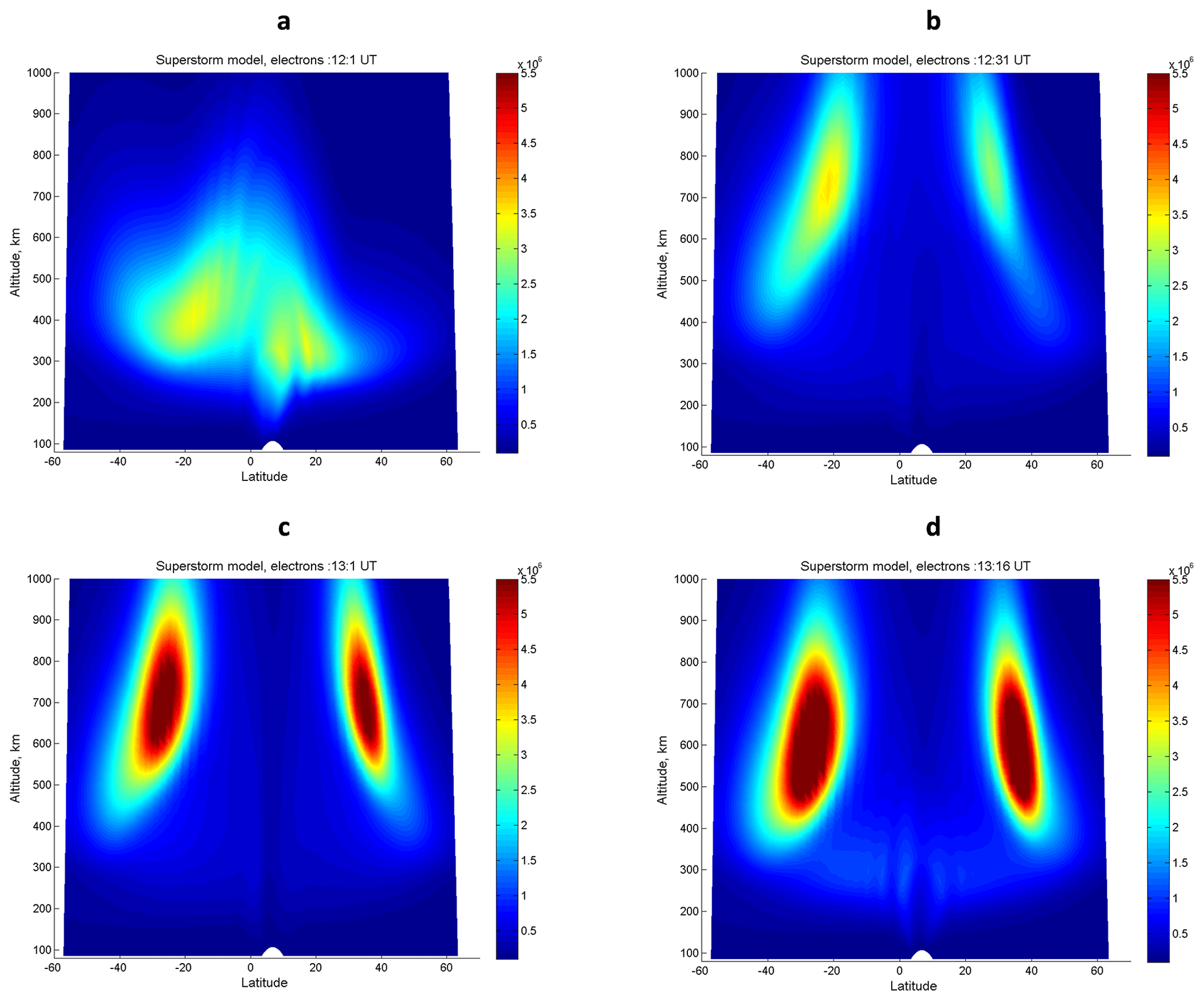
Figure 28A model of the PPEF effects of the Carrington 1859 storm on the dayside ionosphere. The input electric field was taken from Tsurutani et al. (2003) and the simulation was performed using the Huba et al. (2000, 2002) SAMI2 code. The figure is taken from Tsurutani et al. (2012).
Figure 28 shows the SAMI2 results of the modeled dayside ionosphere with ∼20 mV m−1 added to the diurnal variation electric field. The quiet ionosphere is shown in panel (a). The uplift of the O+ ions in both altitude and MLAT after ∼30 min is given in panel (b). The maximum time that the electric field was applied was 1 h. The ionosphere at that time is shown in panel (c). The storm-time equatorial ionospheric anomalies (EIAs) are located at to 40∘ and an altitude of ∼550 to 900 km for the densest portion of the EIAs. Panel (d) shows that the EIAs have come down in altitude but to higher latitudes ∼15 min after the termination of the PPEF application. Parts of the still intense EIAs are now beyond ∘, and now the bulk of the maximum density portion is at ∼400 to 800 km altitude.
It was found that at altitudes of ∼700 to 1000 km, the O+ densities are predicted to be ∼300 times that of the quiet-time neutral densities. It has also been shown by Tsurutani and Lakhina (2014) that in extreme cases, the magnetospheric/ionospheric electric field can be twice as large as the Carrington storm and 6 times as large as the 1991 event. Even if the magnetospheric radiation belt is saturated (there are other scientific papers that state that magnetospheric beta can be greater than 1: Chan et al., 1994; Saitoh et al., 2014; Nishiura et al., 2015), this is a different facet of space weather and the electric field may not be saturated. What will be the ionospheric effects of these even larger electric fields?
A fundamental question for the future is “can the upward O+ ion flow drag sufficient numbers of oxygen neutrals upward so that the oxygen ions plus neutral densities are even higher still?” A short-time interval analytic calculation done by Lakhina and Tsurutani (2017) and a mini-Carrington event modeled by Deng et al. (2018) have indicated that the answer is “yes”. However, a full code needs to be developed and run to answer this question quantitatively. This is an interesting future problem for computer modelers.
Super intense substorms (supersubstorms: SSSs) appear to be externally (solar wind) triggered. Why are they important? They might be the feature within extreme magnetic storms that cause geomagnetically induced currents (GICs)/power outages. This hypothesis needs to be tested.
Figure 29 shows the solar wind data during an intense magnetic storm and two SSSs. From top to bottom are the solar wind speed and density, the magnetic field magnitude and Bz component, and the interplanetary motional electric field, ram pressure and Akasofu epsilon parameter (Perreault and Akasofu, 1978). The bottom two parameters are the SYM-H index and SML index (blue) and the AE index (black). An initial forward shock is indicated by a vertical dashed line at ∼ 05:00 UT, a second shock at ∼ 06:00 UT, and the two SSS onsets by red vertical lines. The criterion for a SSS event was a SML peak value <−2500 nT (an arbitrary number, but chosen to be an extremely high value). At the top of the diagram, the sheath region is indicated by a “Sh” and the magnetic cloud region by “MC”. The first storm main phase is caused by southward Bz in the sheath, and the second, more intense main phase by southward Bz in the MC. The interplanetary magnetic field measurement cadence is 1 min. It has been noted that the magnetosphere typically reacts to southward Bz with durations of >10 to 15 min (Tsurutani et al., 1990), so this high rate of cadence is sufficient to identify any causes of geomagnetic response.
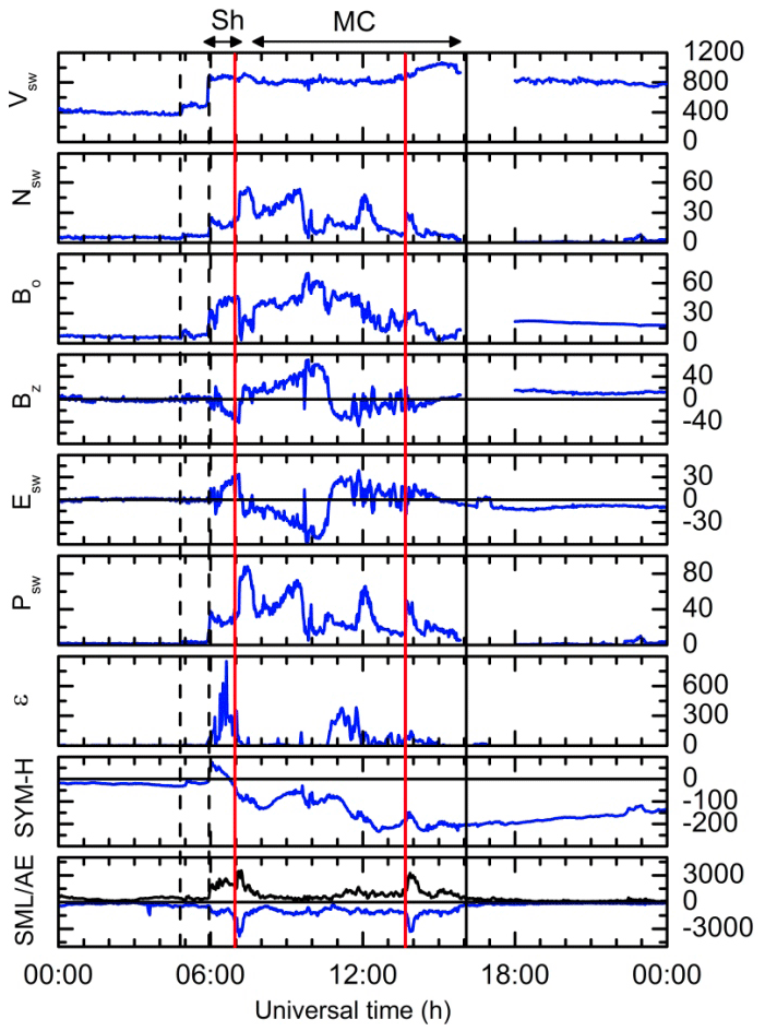
Figure 29Two supersubstorms (SSSs) that occur during a two-phase magnetic storm on 20 November 2001. The onsets of the supersubstorms are indicated by the vertical red lines. The figure is taken from Tsurutani et al. (2015).
It is noted that the SSS events in this case are not triggered at either of the two shocks, nor do they occur during the peak negative SYM-H values of the storm main phases. However, the first SSS event is collocated with a peak Esw and a peak southward Bz of the sheath plasma. The SSS event is also collocated with a large solar wind pressure pulse which is caused by an intense solar wind density feature. The second SSS event occurred in the recovery phase of the second magnetic storm. The IMF Bz was ∼0 nT. The second SSS event was associated with a solar wind pressure pulse associated with a small density enhancement.
A study of SSSs from 1981 to 2012 was conducted by Hajra et al. (2016). In that study a variety of solar wind features were found to be associated with SSS onsets. In that survey it was noted that two SSS events were triggered by fast forward shocks. One of these events will be discussed below.
Figure 30 shows solar wind/interplanetary parameters and geomagnetic parameters during a SSS event on 21 January 2005. From top to bottom are the solar wind speed, density and ram pressure, the magnetic field magnitude and solar wind temperature (in the same panel), the IMF Bz and By components (GSM coordinates), Joule energy and the Akasofu epsilon pressure-corrected parameter ε*, the time-integrated energy input into the magnetosphere and time-integrated Joule energy. The next to bottom panel contains the SYM-H index and the pressure-corrected SYM-H index (SYM-H*). The bottom panel is the SML index. A dashed vertical line denotes the occurrence of a fast forward shock. A vertical solid line indicates the peak of the SSS event.
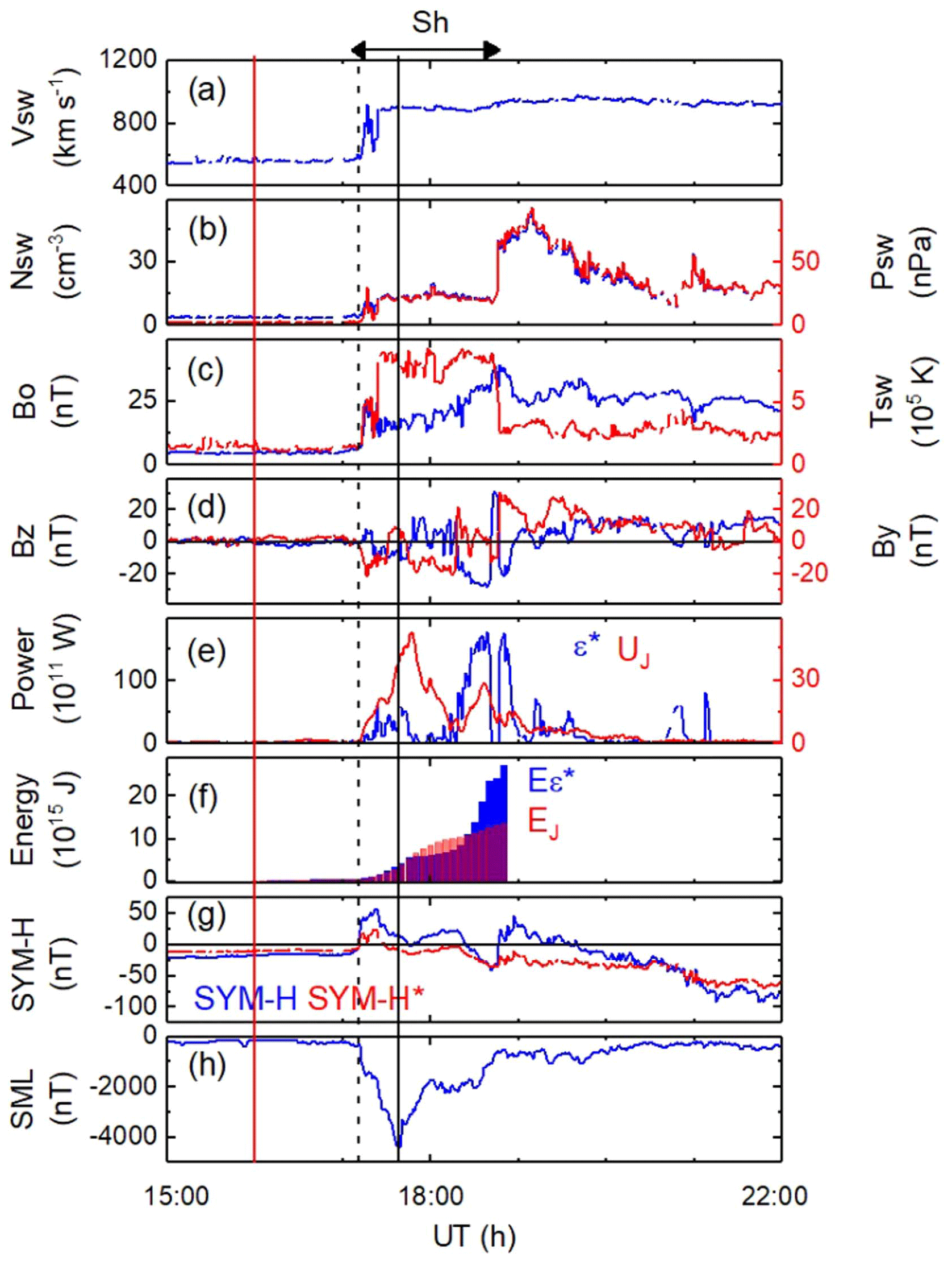
Figure 30An SSS triggered by an interplanetary shock on 21 January 2005. The dashed vertical line indicates a fast forward shock and the solid black line the peak intensity of the SSS event. The figure is taken from Hajra and Tsurutani (2018b).
The SSS event onset at 17:11 UT coincided with a shock with a magnetosonic Mach number of ∼5.5 with a shock normal angle of 81∘. The high-density sheath sunward of the shock causes a SI+ of ∼57 nT. The solar feature associated with this event was an X7 class flare that occurred at ∼ 07:00 UT 20 January (Bombardieri et al., 2008; Saldanha et al., 2008; Pérez-Peraza et al., 2009; Wang et al., 2009; Firoz et al., 2012; Bieber et al., 2013; Tan, 2013). The IMF Bz turned abruptly southward at the time of the shock, so this is part of the energy driving the event. When the IMF Bz turned abruptly northward at ∼ 17:38 UT, the SSS began a recovery phase. This was followed by an interplanetary solar filament (Kozyra et al., 2013), but the latter was not geoeffective in this case. This high plasma density, high magnetic field intensity feature was interpreted by Kozyra et al. (2013) as the interplanetary manifestation of the Illing and Hundhausen (1986) most sunward portion of the three parts of a CME discussed earlier.
Figure 31 contains the Imager for Magnetopause-to-Aurora global Exploration (IMAGE) far-ultraviolet images for the SSS event in Fig. 30. At ∼ 17:13 UT there was a small brightening at ∼68∘ MLAT, which was a very small substorm or pseudo breakup (Elvey, 1957; Tsurutani et al., 1998; Aikio et al., 1999). At ∼ 17:15 UT, 2 min later, there was a ∼ 21:00 MLT premidnight brightening of the aurora at ∼68 to 75∘. At ∼ 17:19 UT the most intense aurora was located at ∼68 to 72∘ in the postmidnight/morning sector, ∼ 00:00 to 04:00 MLT. The aurora moved from a dominant premidnight location to a postmidnight location in ∼4 min.
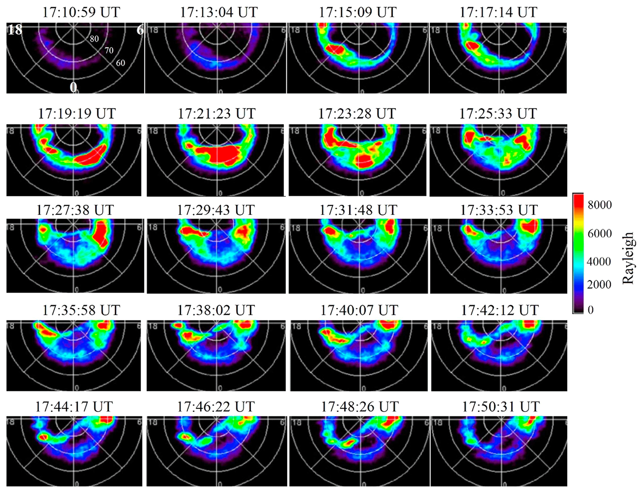
Figure 31IMAGE-FUV images taken from ∼ 17:51 UT on 21 January 2005. These selected auroral images correspond to the SSS event in Fig. 30.
By ∼ 17:26 UT there was almost no aurora of significant intensity at local midnight. At the peak of the SML value at ∼ 17:38 UT until ∼ 17:51, there were both intense premidnight and postmidnight auroras.
The SSS event did not exhibit the Akasofu (1964) standard model of a substorm with an intensification at midnight and then expansion to the west, east and north. The changes in the location of intense auroras were too rapid to track with the IMAGE cadence of ∼2 min.
The SSS events display rapid auroral movements which may entail the appearance of sudden local field-aligned currents. Even smooth motion of auroral forms will cause strong dB∕dt effects over local ground stations. SSS events may be features that can cause GIC effects that have been attributed to “magnetic storms”. Thus, it might be the SSS events within magnetic storms which are the real cause. SWARM satellites are excellently instrumented spacecraft that can study the SSS events in detail and possible resultant GIC effects. However, as noted in the auroral images, there is a need for even higher time resolution global images than is present today. Therefore, it is important to develop and fly auroral UV imagers that can be operated at a ∼1 s cadence in intense auroral substorm events.
We have discussed the current knowledge about various facets of the physics of space weather/solar-terrestrial physics (our thought is that since everything in solar-terrestrial physics is interconnected, it is the same thing as space weather). There are others which we have not touched upon because of limited time and knowledge. The reader should know that other areas of space weather/solar-terrestrial physics exist which may be equally important.
The most critical area for forecasting magnetic storms, either during solar maximum or the declining phase of the solar cycle, is the prediction of the magnetic field Bz and the speed of the convected fields at 1 AU. For CME/MC storms (primarily during solar maximum), this is identifying MC Bz fields near the Sun and understanding the evolution of the MC as it propagates from the Sun to the Earth. This major challenge will be applicable for the prediction of extreme magnetic storms, and hopefully great progress will be made in the next 5 to 10 years. It was shown that for simple MCs for extreme storms one needs to focus on events where the transit time from the Sun to the Earth is less than ∼24 h.
For sheaths upstream of ICMEs during solar maximum and CIRs during the declining phase (CIRs are double sheath structures), the problem is different. Detailed knowledge of the slow solar wind in the space between the Sun and Earth is needed to accurately describe and predict the IMF Bz that impacts the Earth. So far little work has been applied towards predicting the slow solar wind (plus verification). Effort needs to be made in this area to be able to forecast intense to moderate magnetic storms. It was shown that sheath magnetic fields are extremely important for the generation of super intense (Dst<−250 nT) magnetic storms (Meng et al., 2019).
A great deal of knowledge presently exists for establishing SEP events, those energetic particles associated with acceleration at ICME shock fronts (see Luhmann et al., 2017). What is needed for better forecasting is to understand the Mach number of the shocks, the shock normal angles and possibly upstream “seed” particles. The upstream seed particle population is similar to the sheath Bz problem in that this component of the slow solar wind needs to be modeled carefully and accurately. Three spacecraft in the solar wind at different distances from the Sun should help a lot.
The appearance of HSSs at 1 AU is a very tractable problem, that is, if the coronal hole boundaries in the photosphere can be established firmly and the HSS propagation to 1 AU can be done accurately. However, the most difficult task again is the IMF Bz. If Alfvén waves are generated in the interplanetary medium, this will make the task even more difficult. One solution is to measure the interplanetary magnetic field at 1 AU and use filtering techniques (Guarnieri et al., 2018) or again have large apogee Earth orbiters like the IMP-8 spacecraft again. Another possibility is to develop some type of statistical IMF Bz generator. Of course, this technique will only give a ∼30 min to 1 h advanced warning.
Predicting the interplanetary shock Mach numbers and ram pressure jumps will allow foreknowledge of new radiation belt formation, SI+ effects and magnetospheric and ionospheric dB∕dt effects. Dayside auroral intensities and nightside substorm triggering will also be enhanced by predicting incoming shocks.
Several spacecraft missions have been mentioned in relation to some forecasting problems. However, the reader should note that the missions and/or their data alone will not solve these problems. It will either be the scientists on these missions or perhaps totally independent scientists who will make the most progress on these problems. An example is magnetic storms caused by interplanetary shocks/sheaths and CIRs. How long will it take scientists to be able to accurately forecast the time of occurrence of the storm (the easiest part) and the intensity (the hardest part)? Here we will not make an estimate of how long this will take. Shock acceleration of solar flare particles is clearly a fundamental part of space weather. How long will scientists take to be able to predict the fluence and spectral shape at a variety of distances away from the Sun? This is a fundamental problem which space agencies are not currently directly addressing.
A great amount of effort has been put into developing space weather models with the appropriate physics and chemistry included. Some models even use solar and solar wind data and geomagnetic indices that might be useful for short time-duration predictions (Gopalswamy et al., 2001; Srivastava, 2005; Cho et al., 2010; Kim et al., 2010, 2014; Schrijver et al., 2015; Savani et al., 2015). However, in most cases, the usefulness of such models for predictive purposes has not been independently and objectively tested. This needs to be done so that missing physics and chemistry can be applied. When done (testing), surprises might result. It is now being realized that not only the predictability of various models need improvement, but that the level of uncertainty of prediction also needs to be assessed as well (Knipp et al., 2018; Savani et al., 2017).
CME propagation through the interplanetary medium using ENLIL-based codes are making good progress in estimating arrival times of ICMEs at 1 AU and have had varying success in predicting the solar wind parameters as well (Falkenberg et al., 2010; Davis et al., 2011; Pizzo et al., 2015; Jackson et al., 2015; Jian et al., 2015, 2016). However, the fundamental issue of space weather prediction for magnetic storms is the direction and intensity of the magnetic field in both the MC and upstream sheath. These topics still remain a challenge.
Another new approach, the application of machine learning algorithms, is quite promising. For this application, the physics and chemistry need not be known to be applied. Rather the reverse, finding good correlations between solar and interplanetary parameters and magnetospheric observations (for magnetic storms as an example), could lead to a better understanding of the physics, the topic of this paper. But again, one should test these approaches and carefully and objectively assess their accuracy and reliability in making predictions (see Wing et al., 2005, 2016; Reikard, 2015, 2018).
The best test for proving that researchers in space weather understand all of the underlying physics and/or that the machine learning algorithm is robust is to use the program on a new event and see how well it does. This should be done by independent researchers like the people at CCMC at the Goddard Space Research Center, Greenbelt, Maryland, and other facilities.
We have one final comment on a third type of approach to predicting space weather. For atmospheric weather forecasts, the experts down-select to ∼25 of their best codes and run each of the codes with the same input data (Yun et al., 2005; Ruiz et al., 2009; Ghosh and Krishnamurti 2018). The codes produce ∼25 different predictions. The weather service uses the average of the values. Why this scheme works reasonably well is not understood. This may be the final path of space weather forecasting.
Our hope is that the paper is stimulating to the reader in a positive sense: that they will be energized to attack some of the interesting problems in our field of space weather. On the other hand, if the reader finds statements/topics that they disagree with, please send us email comments, and we will try to answer them the best that we can. And if you have disagreements that should see print, Nonlinear Processes in Geophysics has a “Comment” and “Reply” format for discussions of this type.
Partially taken from “From the Sun: Auroras, Magnetic Storms, Solar Flares, Cosmic Rays” (Suess and Tsurutani, 1998, AGU Press)
Adiabatic invariant. In a nearly collisionless, ionized gas, electrically charged particles orbit around magnetic lines of force. Certain physical quantities are approximately constant for slow (adiabatic) changes in the magnetic field in time or in space, and these quantities are called adiabatic invariants. For example, the magnetic moment of a charged particle, , is such a constant, where V⊥ is the velocity of the particle perpendicular to the magnetic field, B is the magnetic field strength, and m is the particle mass. In a converging field such as in approaching the pole of a magnetic dipole, the field strength increases and therefore V⊥ increases as well because μ has to remain constant.
Aeronomy. The science of the (upper) regions of atmospheres, those regions where dissociation of molecules and ionization are present.
Alfvén wave (magnetohydrodynamic shear wave). A transverse wave in magnetized plasma characterized by a change in direction of the magnetic field with no change in either the intensity of the field or the plasma density.
Anisotropic plasma. A plasma whose properties vary with direction relative to the ambient magnetic field direction. This can be due, for example, to the presence of a magnetic or electric field. See also Isotropic plasma and Plasma.
Arase satellite, formerly called Exploration of energization and Radiation in Geospace or ERG. A scientific satellite developed by the Institute of Space and Astronautical Science (ISAS) of the Japanese Aerospace Exploration Agency (JAXA) to study the Van Allen radiation belts.
Astronomical unit (AU). The mean radius of the Earth's orbit, 1.496×1013 cm.
Aurora. A visual phenomenon that occurs mainly in the high-latitude night sky. Auroras occur within a band of latitudes known as the auroral oval, the location of which is dependent on the intensity of geomagnetic activity. Auroras are a result of collisions between precipitating charged particles (mostly electrons) and atmospheric atoms and molecules, exciting the atmospheric constituents. The charged particles come from the outer parts of the magnetosphere and are guided by the geomagnetic field. Each gas (oxygen and nitrogen molecules and atoms) emits its own characteristic radiation when bombarded by the precipitating particles. Since the atmospheric composition varies with altitude and the faster precipitating particles penetrate deeper into the atmosphere, certain auroral colors originate preferentially from certain heights in the sky. The auroral altitude range is 80 to 500 km, but typical auroras occur 90 to 250 km above the ground. The color of the typical aurora is yellow–green, from a specific transition line of atomic oxygen. Auroral light from lower levels in the atmosphere is dominated by blue and red bands from molecular nitrogen and molecular oxygen. Above 250 km, auroral light is characterized by a red spectral line of atomic oxygen. To an observer on the ground, the combined light of these three fluctuating primary colors produces an extraordinary visual display. Auroras in the Northern Hemisphere are called the aurora borealis or “northern lights”. Auroras in the Southern Hemisphere are called the aurora australis. The patterns and forms of the aurora include quiescent “arcs”, rapidly moving “rays” and “curtains”, “patches”, and “veils”.
Auroral electrojet (AE). See Electrojet. Auroral oval: an elliptical band around each geomagnetic pole ranging from about 75∘ magnetic latitude at local noon to about 67∘ magnetic latitude at midnight under average conditions. It is the locus of those locations of the maximum occurrence of auroras and widens to both higher and lower latitudes during the expansion phase of a magnetic substorm.
Beta (e.g., low-beta plasma). The ratio of the thermal pressure to the magnetic “pressure” in a plasma – in centimeter gram second (c.g.s.).
Bow shock (Earth, heliosphere). A collisionless shock wave in front of the magnetosphere arising from the interaction of the supersonic solar wind with the Earth's magnetic field. An analogous shock is the heliospheric bow shock which exists in front of the heliosphere and is due to the interaction of the interstellar wind with the solar wind and the interplanetary magnetic field.
Charge exchange. An interaction between a charged particle and a neutral atom wherein the charged particle becomes neutral and the neutral particle becomes charged through the exchange of an electron.
Cloud (magnetic). See Magnetic cloud.
Collisional (de-)excitation. Excitation of an atom or molecule to a higher energy state due to a collision with another atom, molecule, or ion. The higher energy state generally refers to electrons in higher energy around atoms. De-excitation is the reduction of a higher electron energy state to a lower one, usually accomplished by a collision with another atom, molecule or ion.
Convection (magnetospheric, plasma, thermal). The bulk transport of plasma (or gas) from one place to another, in response to mechanical forces (for example, viscous interaction with the solar wind) or electromagnetic forces. Thermal convection, due to heating from below and the gravitational field, is what drives convection inside the Sun. Magnetospheric convection is driven by the dragging of the Earth's magnetic field and plasma together by the solar wind when the magnetic field becomes attached to the magnetic field in the solar wind.
Coriolis force. In the frame of a rotating body (such as the Earth), a force due to the bodily rotation. All bodies that are not acted upon by some force have the tendency to remain in a state of rest or of uniform rectilinear motion (Newton's first law), so that this force is called a “fictitious” force. It is a consequence of the continuous acceleration which must be applied to keep a body at rest in a rotating frame of reference.
Corona. The outermost layer of the solar atmosphere, characterized by low densities (<109 cm3 or 1015 m−3) and high temperatures (>106 K).
Coronal hole. An extended region of the solar corona characterized by exceptionally low density and in a unipolar photospheric magnetic field with “open” magnetic field topology. Coronal holes are largest and most stable at or near the solar poles and are a source of high-speed (700–800 km s−1) solar wind. Coronal holes are visible at several wavelengths, most notably solar X-rays visible only from space, but also in the He 1083 nm line which is detectable from the surface of the Earth. In soft X-ray images (photon energy of ∼0.1–1.0 keV or a wavelength of 10–100 Å), these regions are dark, hence the name “holes”.
Coronal mass ejection (CME). A transient outflow of plasma from or through the solar corona. CMEs are often but not always associated with erupting prominences, disappearing solar filaments, and flares.
Corotation (with the Earth). A plasma in the magnetosphere of the Earth is said to be corotating with the Earth if the magnetic field drags the plasma with it and together they have a 24 h rotation period.
Cosmic ray (galactic, solar). Extremely energetic (relativistic) charged particles or electromagnetic radiation, primarily originating outside of the Earth's magnetosphere. Cosmic rays usually interact with the atoms and molecules of the atmosphere before reaching the surface of the Earth. The nuclear interactions lead to formation of daughter products, and they in turn to granddaughter products, etc. Thus, there is a chain of reactions and a “cosmic ray shower”. Some cosmic rays come from outside the solar system, while others are emitted from the Sun in solar flares. See also Anomalous cosmic ray, Energetic particle, and Solar energetic particle (SEP) event.
Constellation Observing System for Meteorology, Ionosphere and Climate-2 (COSMIC II). A joint Taiwan National Space Organization (NSPO)–US National Oceanic and Atmospheric Administration (NOAA) mission of six satellites in low-inclination orbit to study the Earth's ionosphere.
Corotating interaction region (CIR). An interplanetary region of high magnetic fields and plasma densities created by the interaction of a high-speed solar wind stream with the upstream slow solar wind. The antisunward portion of the CIR is compressed slow solar wind plasma and magnetic fields, and the sunward portion is compressed fast solar wind plasma and magnetic fields. The two regions of the CIR are separated by a tangential discontinuity.
Cyclotron frequency. When a particle of charge q moves in a magnetic field B, the particle orbits or gyrates around the magnetic field lines. The cyclotron frequency is the frequency of this gyration and is given by , where m is the mass of the particle, and c is the velocity of light (in centimeter gram second (c.g.s.) units).
Cyclotron resonance. The frequency at which a charged particle experiences a Doppler-shifted wave at the particle's cyclotron frequency. Because the particle and wave may be traveling at different speeds and in different directions, there is usually a Doppler shift involved.
D region. A daytime region of the Earth's ionosphere beginning at approximately 40 km, extending to 90 km altitude. Radio wave absorption in this region can be significantly increased due to increasing ionization associated with the precipitation of solar energetic particles through the magnetosphere and into the ionosphere.
Diffusion. The slow, stochastic motion of particles.
Diffusive shock acceleration. Charged particle acceleration at a collisionless shock due to stochastic scattering processes caused by waves and plasma turbulence. See also Shock wave (collisionless).
Dipole magnetic field. A magnetic field whose intensity decreases as the cube of the distance from the source. A bar magnet's field and the magnetic field originating in the Earth's core are both approximately dipole magnetic fields.
Drift (of ions/electrons). As particles gyrate around magnetic field lines, their orbits may “drift” perpendicularly to the local direction of the magnetic field. This occurs if there is a force also perpendicular to the field, e.g., an electric field, curvature in the magnetic field direction, or gravity.
Driver gas. A mass of plasma and entrained magnetic field that is ejected from the Sun and has a velocity higher than the upstream plasma and “drives” a (usually collisionless) shock wave ahead of itself. The magnetic cloud within an ICME is the same thing as a driver gas.
Dst index. A measure of variation in the geomagnetic field due to the equatorial ring current. It is computed from the H components at approximately four near-equatorial stations at hourly intervals. At a given time, the Dst index is the average of variation over all longitudes; the reference level is set so that Dst is statistically zero on internationally designated quiet days. An index of −50 nT (nanoTesla) or less indicates a storm-level disturbance, and an index of −200 nT or less is associated with middle-latitude auroras. Dst is determined by the World Data Center C2 for Geomagnetism, Kyoto University, Kyoto, Japan.
Dynamo (solar magnetospheric). The conversion of mechanical energy (rotation in the case of the Sun) into electrical current. This is the process by which magnetic fields are amplified by the induction of plasmas being forced to move perpendicular to the magnetic field lines. See also Mean field electro-dynamics.
E region. A daytime region of the Earth's ionosphere roughly between the altitudes of 90 and 160 km. The E-region characteristics (electron density, height, etc.) depend on the solar zenith angle and the solar activity. The ionization in the E layer is caused mainly by X-rays in the range 0.8 to 10.4 nm coming from the Sun.
Ecliptic plane. The plane of the Earth's orbit about the Sun. It is also the Sun's apparent annual path, or orbit, across the celestial sphere.
Electrically charged particle. Electrons and protons, for example, or any atom from which electrons have been removed to make it into a positively charged ion. The elemental charge of particles is esu. An electron and a proton have this charge. Combined (a hydrogen atom), the charge is zero. Ions have multiples of this charge, depending on the number of electrons which have been removed (or added).
Electrojet. (1) Auroral electrojet (AE): a current that flows in the ionosphere at a height of ∼100 km in the auroral zone. (2) Equatorial electrojet: a thin electric current layer in the ionosphere over the dip equator at about 100 to 115 km altitude.
Electron plasma frequency/wave. The natural frequency of oscillation of electrons in a neutral plasma (e.g., equal numbers of electrons and protons).
Electron Volt (eV). The kinetic energy gained by an electron or proton being accelerated in a potential drop of 1 V.
ESA. European Space Agency
Extreme Ultraviolet (EUV). A portion of the electromagnetic spectrum from approximately 10 to 100 nm.
Extremely low frequency (ELF). That portion of the radio frequency spectrum from 30 to 3000 Hz.
Fast mode (wave/speed). In magnetohydrodynamics, the fastest wave speed possible. Numerically, this is equal to the square root of the sum of the squares of the Alfvén speed and plasma sound speed.
Field-aligned current. A current flowing along (or opposite to) the magnetic field direction.
Filament. A mass of gas suspended over the chromosphere by magnetic fields and seen as dark ribbons threaded over the solar disk. A filament on the limb of the Sun seen in emission against the dark sky is called a prominence. Filaments occur directly over magnetic-polarity inversion lines, unless they are active.
Flare. A sudden eruption of energy in the solar atmosphere lasting minutes to hours, from which radiation and energetic charged particles are emitted. Flares are classified on the basis of area at the time of maximum brightness in H alpha.
-
Importance 0 (subflare). <2.0 hemispheric square degrees
-
Importance 1. 2.1–5.1 square degrees
-
Importance 2. 5.2–12.4 square degrees
-
Importance 3. 12.5–24.7 square degrees
-
Importance 4. >=24.8 square degrees (1 square degree is equal to (1.214×10⁴ km) squared = 48.5 millionths of the visible solar hemisphere.)
-
A brightness qualifier F, N, or B is generally appended to the importance character to indicate faint, normal, or brilliant (for example, 2B).
Flux rope. A magnetic phenomenon which has a force-free field configuration.
Force-free field. A magnetic field which exerts no force on the surrounding plasma. This can either be a field with no flowing electrical currents or a field in which the electrical currents all flow parallel to the field.
Free energy (of a plasma). When an electron or ion distribution is either non-Maxwellian or anisotropic, they are said to have “free energy” from which plasma waves can be generated via instabilities. The waves scatter the particles so they become more isotropic, reducing the free energy.
Frozen-in field. In a tenuous, collisionless plasma, the weak magnetic fields embedded in the plasma are convected with the plasma; i.e., they are “frozen in”.
Galactic cosmic ray (GCR). See Cosmic ray.
Gamma ray. Electromagnetic radiation at frequencies higher than X-rays.
Geomagnetic storm. A worldwide disturbance of the Earth's magnetic field, distinct from regular diurnal variations. A storm is precisely defined as occurring when DsT becomes less than −50 nT (see geomagnetic activity).
Geomagnetically induced currents (GICs). Currents flowing along electric power transmission systems and other electrically conducting infrastructures are produced by naturally induced geoelectric fields during geomagnetic disturbances.
Geosynchronous orbit. Term applied to any equatorial satellite with an orbital velocity equal to the rotational velocity of the Earth. The geosynchronous altitude is near 6.6 Earth radii (approximately 36 000 km above the Earth's surface). To be geostationary as well, the satellite must satisfy the additional restriction that its orbital inclination be exactly 0 ∘. The net effect is that a geostationary satellite is virtually motionless with respect to an observer on the ground.
GeV. 109 electron Volts (Giga-electron Volt).
Global Navigation Satellite System (GNSS). GNSS receivers use the orbiting satellite Global Positioning System (GPS) transmitted signals to obtain the geographic location of a user's receiver anywhere in the world.
The Global Positioning System (GPS) is a global navigation satellite system that provides geolocation and time information to a GPS receiver anywhere on or near the Earth where there is an unobstructed line of sight to four or more GPS satellites.
Global-scale Observations of the Limb and Disk (GOLD). A NASA mission to “investigate the dynamic intermingling of space and Earth's uppermost atmosphere” (https://www.nasa.gov/feature/goddard/2018/nasa-gold-mission-to-image-earth-s-interface-to-space).
Heliosphere. The magnetic cavity surrounding the Sun, carved out of the galaxy by the solar wind.
Heliospheric current sheet (HCS). This is the surface dividing the northern and southern magnetic field hemispheres in the solar wind. The magnetic field is generally one polarity in the north and the opposite in the south, so just one surface divides the two polarities. However, the Sun's magnetic field changes over the 11-year solar sunspot cycle and reverses polarity at solar maximum. The same thing happens in the magnetic field carried away from the Sun by the solar wind so the HCS only lies in the equatorial near-solar minimum. It is called a “current sheet” because it carries an electrical current to balance the oppositely directed field on either side of the surface. It is very thin on the scale of the solar system – usually only a few proton gyroradii, or less than 100 000 km.
Helmet streamer. See Streamer.
Heliospheric plasma sheet (HPS). A high-density slow solar wind region that is located adjacent to the heliospheric current sheet (HCS).
High frequency (HF). That portion of the radio frequency spectrum between 3 and 30 MHz.
High-speed solar wind (HSS). A solar wind with speeds of 750 to 800 km s−1 emanating from solar coronal holes. The HSS is characterized by embedded, particularly large-amplitude Alfvén waves. At the edges of HSSs, the velocities can be less due to superradial expansion effects.
Instability. When an electron or ion distribution is sufficiently anisotropic, it becomes unstable (instability), generating plasma waves. The anisotropic distribution provides a source of free energy for the instability. A simple analog is a stick, which if stood on its end is “unstable” but which if laid on its side is “stable”. In this analog, gravity pulls on the stick and provides a source of free energy when the stick is stood on its end.
Interplanetary magnetic field (IMF, Parker spiral). The magnetic field carried with the solar wind and twisted into an Archimedean spiral by the Sun's rotation.
Interplanetary medium. The volume of space in the solar system that lies between the Sun and the planets. The solar wind flows in the interplanetary medium.
Interplanetary coronal mass ejection (ICME). The evolutionary part of a CME as it propagates through interplanetary space. Typically, after the CME has propagated 1 AU from the Sun, the ICME only contains the magnetic cloud (MC) portion of the initial three parts of a CME. The MC may also have been compressed/expanded or rotated by the time it reaches 1 AU.
Interplanetary shock. A fast forward shock is characterized by a sharp increase in solar wind speed, plasma density, plasma temperature and magnetic field magnitude. The shock reduces the upstream plasma from a supermagnetosonic state to a subsonic state, much as an airplane wing sonic shock reduces the relative flow of air from a supersonic speed (relative to the airplane) to a subsonic speed. A fast (magnetosonic) forward (propagating in the direction of the “piston”, in this case the propagation of the ICME in the anti-solar direction) shock is detected upstream (antisolarward) of fast ICMEs. A reverse shock propagates in the direction of the Sun. Planetary bow shocks are reverse shocks. There are other types of shocks not discussed in this paper: slow shocks and intermediate shocks.
Interstellar (gas, neutral gas, ions, cosmic rays, wind, magnetic field, etc.). Literally, between the stars. In practical terms, it is anything beyond the outer boundary of the solar wind (the “heliopause”) yet within the Milky Way.
Ion. (1). An electrically charged atom or molecule. (2). An atom or molecular fragment that has a positive electrical charge due to the loss of one or more electrons; the simplest ion is the hydrogen nucleus, a single proton.
Ionization state. The number of electrons missing from an atom.
Ionosphere. The region of the Earth's upper atmosphere containing free (not bound to an atom or molecule) electrons and ions. This ionization is produced from the neutral atmosphere by solar ultraviolet radiation at very short wavelengths (<100 nm) and also by precipitating energetic particles.
Ionospheric storm. A positive ionospheric storm is where the ionospheric total electron content (TEC) increases. A negative ionospheric storm is an event where the ionospheric TEC decreases.
Ionospheric Connection Explorer (ICON) is a NASA 2-year mission that will give new views of the boundary between our atmosphere and space, where planetary weather and space weather meet.
Irradiance. Radiant energy flux density on a given surface (e.g., ergs cm−2 s−1)
keV. One thousand electron Volts (kiloelectron Volt). See Electron Volt. See also Anisotropic plasma and Plasma.
L value. For a dipole magnetic field, the field line that crosses the magnetic equator at an L value equal to the number in Earth radii.
Loop (solar-loop prominence system). A magnetic loop is the flux tube which crosses from one polarity to another. A loop prominence bridges a magnetic inversion line across which the magnetic field changes direction. See also Magnetic foot point and Prominence.
Loss cone. A small cone angle about the ambient magnetic field direction where magnetospheric charged particles with velocity vectors within the cone will mirror at sufficiently low altitudes such that the particle will have collisions with atmospheric atoms and molecules and will be “lost” from returning to the magnetosphere.
Loss cone instability. An instability generated by a plasma anisotropy where the temperature perpendicular to the magnetic field is greater than the temperature parallel to the field. This instability gets its name because this condition exists in the Earth's magnetosphere and the “loss cone” particles are those that are lost into the upper atmosphere.
Magnetic cloud. A region in the solar wind of about 0.25 AU or more in radial extent in which the magnetic field strength is high and the direction of one component of the magnetic field changes appreciably by means of a rotation nearly parallel to a plane. Magnetic clouds may be parts of the driver gases (coronal mass ejections) in the interplanetary medium.
Magnetic foot point. For the Earth's magnetic field lines, where the magnetic field enters the surface of the Earth.
Magnetic mirror. Charged particles moving into a region of converging magnetic flux (as at the pole of a magnet) will experience Lorentz forces that slow the particles and “mirror” them by eventually reversing their direction if the particles are initially moving slowly enough along the field line. See also Mirror point.
Magnetic reconnection. The act of interconnection between oppositely directed magnetic field lines. Magnetic reconnection is recognized as a basic plasma process, which converts magnetic energy into plasma kinetic energy accompanied by topological changes in the magnetic field configuration. It does not allow an excessive buildup of magnetic energy in the current sheets.
Magnetic storm. See Geomagnetic storm.
Magnetopause. The boundary surface between the solar wind and magnetosphere, where the pressure of the magnetic field of the object effectively equals the ram pressure of the solar wind plasma.
Magnetosheath. The region between the bow shock and the magnetopause, characterized by very turbulent plasma. This plasma has been heated (shocked) and slowed as it passed through the bow shock. For the Earth, along the Sun–Earth axis, the magnetosheath is about 3 Earth radii thick.
Magnetosonic speed (acoustic speed). The speed of the fastest low-frequency magnetic waves in a magnetized plasma. It is the equivalent of the sound speed in a neutral gas or non-magnetized plasma.
Magnetosphere. The magnetic cavity surrounding a magnetized planet, carved out of the passing solar wind by virtue of the planetary magnetic field, which prevents, or at least impedes, the direct entry of the solar wind plasma into the cavity.
Magnetospheric Multiscale Mission (MMS). A NASA mission designed to spend extensive periods in locations where magnetic reconnection at the magnetopause/magnetotail is expected to occur. The critical electron diffusion region will be studied. The mission consists of four spacecraft flown in a tetrahedron configuration.
Magnetotail. The extension of the magnetosphere in the antisunward direction as a result of interaction with the solar wind. In the inner magnetotail, the field lines maintain a roughly dipolar configuration. But at greater distances in the antisunward direction, the field lines are stretched into northern and southern lobes, separated by a plasma sheet. There is observational evidence of traces of the Earth's magnetotail as far as 1000 Earth radii downstream, in the anti-solar direction.
Main phase. Of a geomagnetic storm, that period when the horizontal magnetic field at middle latitudes decreases, owing to the effects of an increasing magnetospheric ring current. The main phase can last for hours, but typically lasts less than 1 d.
Maxwellian distribution. The minimum energy particle distribution for a given temperature. It is also the equilibrium distribution in the absence of losses due to radiation, collisions, etc.
Mean free path. The statistically most probably distance a particle travels before undergoing a collision with another particle or interacting with a wave.
Mesosphere. The region of the Earth's atmosphere between the upper limit of the stratosphere (approximately 30 km altitude) and the lower limit of the thermosphere (approximately 80 km altitude).
MeV. One million electron Volts (Megaelectron Volt). See also Electron Volt.
Mirror point. The point where the charged particles reverse direction (mirrors). At this point, all of the particle motion is perpendicular to the local ambient magnetic field. See also Magnetic mirror.
Parker Solar Probe. A NASA robotic spacecraft to probe the outer corona of the Sun. It will approach to within 9.9 solar radii (6.9 million kilometers or 4.3 million miles from the center of the Sun) and will travel, at closest approach, as fast as 690 000 km h−1 (430 000 mph).
Photosphere. The lowest visible layer of the solar atmosphere; it corresponds to the solar surface viewed in white light. Sunspots and faculae are observed in the photosphere.
Pickup ion. This is called a pickup ion because as soon as the neutral atom is ionized and the plasma velocity is orthogonal to the embedded magnetic field, the ion becomes attached to the magnetic field and is carried by the plasma and so is “picked up”. If the magnetic field is oriented parallel to the plasma flow direction, a plasma instability results and waves scatter the particles until they are picked up.
Pitch angle. In a plasma, the angle between the instantaneous velocity vector of a charged particle and the direction of the ambient magnetic field.
Plasma (ions, electrons). A gas that is sufficiently ionized so as to affect its dynamical behavior. A plasma is a good electrical conductor and is strongly affected by magnetic fields. See also Anisotropic plasma and Isotropic plasma.
Plasma instability (ion, electron). When a plasma is sufficiently anisotropic, plasma waves grow, which in turn alter the distribution via wave–particle interactions. The plasma is “unstable”.
Plasma sheet. A region in the center of the magnetotail between the northern and southern lobes. The plasma sheet is characterized by hot, dense plasma and is a high-beta plasma region, in contrast to the low-beta lobes. The plasma sheet bounds the neutral sheet where the magnetic field direction reverses from earthward (northern lobe direction) to anti-earthward (southern lobe direction).
Plasma wave (electrostatic/electromagnetic). A wave generated by plasma instabilities or other unstable modes of oscillation allowable in a plasma. “Chorus” and “Plasmaspheric hiss” are whistler wave modes. These are electromagnetic waves with frequencies below the electron cyclotron frequency. Electromagnetic ion cyclotron (EMIC) waves are ion cyclotron waves with frequencies below the proton cyclotron frequency.
Polar cap absorption event (PCA). An anomalous condition of the polar ionosphere whereby HF and VHF (3–300 MHz) radio waves are absorbed and LF and VLF (3–300 kHz) radio waves are reflected at lower altitudes than normal. The cause is energetic particle precipitation into the ionosphere/atmosphere. The enhanced ionization caused by this precipitation leads to cosmic radio noise absorption and attenuation of that noise at the surface of the Earth. PCAs generally originate with major solar flares, beginning within a few hours of the event (after the flare particles have propagated to the Earth) and maximizing within a day or 2 after onset. As measured by a riometer (relative ionospheric opacity meter), the PCA event threshold is 2 dB of absorption at 30 MHz for daytime and 0.5 dB at night. In practice, the absorption is inferred from the proton flux at energies greater than 10 MeV, so that PCAs and proton events are simultaneous. However, the transpolar radio paths may still be disturbed for days, up to weeks, following the end of a proton event, and there is some ambiguity about the operational use of the term PCA.
Prominence. A term identifying cloud-like features in the solar atmosphere. The features appear as bright structures in the corona above the solar limb and as dark filaments when seen projected against the solar disk. Prominences are further classified by their shape (for example, mound prominence, coronal rain) and activity. They are most clearly and most often observed in H alpha. See also Loop.
Radiation belt. Regions of the magnetosphere roughly 1.2 to 6 Earth radii above the equator in which charged particles are stably trapped by closed geomagnetic field lines. There are two belts. The inner belt's maximum proton density lies near 5000 km above the Earth's surface. Inner belt protons (10s of MeV) and electrons (100s of keV) originate from the decay of secondary neutrons created during collisions between cosmic rays and upper atmospheric particles. The outer belt extends on to the magnetopause on the sunward side (10 Earth radii under normal quiet conditions) and to about 6 Earth radii on the nightside. The altitude of maximum proton density is near 16 000–20 000 km. Outer belt protons and electrons are lower energy (about 200 eV to 1 MeV). The origin of the particles (before they are energized to these high energies) is a mixture of the solar wind and the ionosphere. The outer belt is also characterized by highly variable fluxes of energetic electrons. The radiation belts are often called the “Van Allen radiation belts” because they were discovered in 1958 by a research group at the University of Iowa led by Professor J. A. Van Allen. See also Trapped particle.
Ram pressure. Sometimes called “dynamic pressure”. The pressure exerted by a streaming plasma upon a blunt object.
Reconnection. A process by which differently directed field lines link up, allowing topological changes in the magnetic field to occur, determining patterns of plasma flow and resulting in conversion of magnetic energy to kinetic and thermal energy of the plasma. Reconnection is invoked to explain the energization and acceleration of the plasmas/energetic particles that are observed in solar flares, magnetic substorms and storms, and elsewhere in the solar system.
Recovery phase. Of a geomagnetic storm, that period when the depressed northward field component returns to normal levels. Recovery is typically complete in 1 to 2 d.
Relativistic. Charged particles (ions or electrons) which have speeds comparable to the speed of light.
RHESSI. The Reuven Ramaty High Energy Solar Spectroscopic Imager was a NASA solar flare observatory. It was launched on 5 February 2002 and was operational until 16 Auguust 2018. RHESSI's primary mission was to explore the physics of particle acceleration and energy release in solar flares.
Ring current. In the magnetosphere, a region of current that flows near the geomagnetic equator in the outer belt of the two Van Allen radiation belts. The current is produced by the gradient and curvature drift of the trapped charged particles of energies of 10 to 300 keV. The ring current is greatly augmented during magnetic storms because of the hot plasma injected from the magnetotail and upwelling oxygen ions from the ionosphere. Further acceleration processes bring these ions and electrons up to ring current energies. The ring current (which is a diamagnetic current) causes a worldwide depression of the horizontal geomagnetic field during a magnetic storm.
SDO/EVE. The Solar Dynamics Observatory is a NASA mission designed to understand the Sun's influence on the Earth and near-Earth space by studying the solar atmosphere on small scales of space and time at many wavelengths simultaneously. The EVE (Extreme Ultraviolet Variability Experiment) instrument measures the solar extreme ultraviolet (EUV) spectral irradiance at high spectral resolution, temporal cadence and precision.
Solar energetic particle (SEP). An energetic particle of solar flare/interplanetary shock origin.
Sheath. The plasma and magnetic fields in the downstream subsonic region after collisionless shocks. See Shock wave.
Shock wave. A shock wave is characterized by a discontinuous change in pressure, density, temperature, and particle streaming velocity, propagating through a compressible fluid or plasma. Fast collisionless shock waves occur in the solar wind when fast solar wind overtakes slow solar wind, with the difference in speeds being greater than the magnetosonic speed. Collisionless shock thicknesses are determined by the proton and electron gyroradii rather than the collision lengths. See also Diffusive shock acceleration and Solar wind shock.
Solar corona. See Corona.
Solar cycle. The approximately 11-year quasi-periodic variation in the sunspot number. The polarity pattern of the magnetic field reverses with each cycle. Other solar phenomena, such as the 10.7 cm solar radio emission, exhibit similar cyclical behavior. The solar magnetic field reverses each sunspot cycle, so there is a corresponding 22-year solar magnetic cycle.
Solar energetic particle (SEP) event. A high-flux event of solar (low-energy) cosmic rays. This is commonly generated by larger solar flares or CME shocks and lasts typically from minutes to days. See also Cosmic ray.
Solar flares. Transient perturbations of the solar atmosphere as measured by enhanced X-ray emission (see X-ray flare class), typically associated with flares. Five standard terms are used to describe the activity observed or expected within a 24 h period.
-
Very low – X-ray events less than C class
-
Low – C-class X-ray events
-
Moderate – isolated (one to four) M-class X-ray events
-
High – several (five or more) M-class X-ray events, or isolated (one to four)
-
M5 or greater X-ray events
-
Very high – several (five or more) M5 or greater X-ray events
Solar maximum. The month(s) during the sunspot cycle when the smoothed sunspot number reaches a maximum.
Solar minimum. The month(s) during the sunspot cycle when the smoothed sunspot number reaches a minimum.
Solar Orbiter. A European Space Agency-led (ESA) mission intended to perform detailed measurements of the inner heliosphere and nascent solar wind to answer the question “How does the Sun create and control the heliosphere?”. The mission will make observations of the Sun from an eccentric orbit moving as close as ∼60 solar radii (RS) or 0.284 astronomical units (AU) from the Sun.
Solar wind. The outward flow of solar particles and magnetic fields from the Sun. Typically at 1 AU, solar wind velocities are 300–800 km s−1 and proton and electron densities are 3–7 per cubic centimeter (roughly inversely correlated with velocity). The total intensity of the interplanetary magnetic field is nominally 3–8 nT.
SORCE. Solar Radiation and Climate Experiment. A NASA mission that measures electromagnetic radiation produced by the Sun and the power per unit area of that energy on the Earth's surface.
Space weather. Dynamic variations at the Sun, in interplanetary space, in the Earth's and planetary magnetospheres, ionospheres and atmospheres associated with space phenomena.
Stratosphere. That region of the Earth's atmosphere between the troposphere and the mesosphere. It begins at an altitude of temperature minimum at approximately 13 km and defines a layer of increasing temperature up to about 30 km.
Streamer. A feature of the white light solar corona (seen in eclipse or with a coronagraph) that looks like a ray extending away from the Sun out to about 1 solar radius, with an arch-like base containing a cavity usually occupied by a prominence.
Substorm. A substorm corresponds to an injection of charged particles from the magnetotail into the nightside magnetosphere. Plasma instabilities lead to the precipitation of the particles into the auroral zone ionosphere, producing intense auroras. Potential drops along magnetic field lines lead to the acceleration of ∼1 to 10 keV electrons with brilliant displays of auroras as the electrons impact the upper atmosphere. Enhanced ionospheric conductivity and externally imposed electric fields lead to the intensification of the auroral electrojets.
Sudden impulse (SI). An abrupt (10s of seconds) jump in the Earth's surface magnetic field. The positive sudden impulses (SI+s) are caused by fast forward shock impingement onto the magnetosphere.
Sunspot. An area seen as a dark spot, in contrast to its surroundings, on the photosphere of the Sun. Sunspots are concentrations of magnetic flux, typically occurring in bipolar clusters or groups. They appear dark because they are cooler than the surrounding photosphere. Larger and darker sunspots sometimes are surrounded (completely or partially) by penumbrae. The dark centers are umbrae. The smallest, immature spots are sometimes called pores.
Supersubstorm. Defined as an event with SML<−2500 nT. These auroral zone events appear to have different evolutionary properties than the standard (Akasofu, 1964) auroral substorms.
SWARM. A European Space Agency (ESA) mission originally instrumented to study the Earth's magnetic field. The current goals are to study magnetospheric–ionospheric coupling and auroral space weather problems.
Tesla. A unit of magnetic flux density (Weber/m2). A nanoTesla (nT) is 10−9 Teslas.
Termination shock. The shock wave in the solar wind which is caused by the abrupt deceleration of the solar wind as it runs into the local interstellar medium (LISM). It is thought to lie somewhere between 70 and 150 AU from the Sun.
Thermal speed (ion, electron). The random velocity of a particle associated with its temperature.
Thermosphere. That region of the Earth's atmosphere where the neutral temperature increases with height. It begins above the mesosphere at about 80–85 km and extends upward to the exosphere.
TIMED. Thermosphere Ionosphere Mesosphere Energetics and Dynamics. A NASA mission to investigate and understand the energetics of the Earth's mesosphere and lower thermosphere/ionosphere.
Total electron content (TEC). The column density of electrons in the Earth's ionosphere.
Trapped particle. Particles gyrating about magnetic field lines (e.g., in the Earth's magnetosphere). See also Magnetic mirror and Pitch angle.
Troposphere. The lowest layer of the Earth's atmosphere, extending from the ground to the stratosphere, approximately 13 km in altitude. In the troposphere, temperature decreases with height.
Ultraviolet (UV). That part of the electromagnetic spectrum between 5 and 400 nm.
Ultra low frequency (ULF). One milliHertz to 1 Hz.
Very high frequency (VHF). That portion of the radio frequency spectrum from 3 to 300 MHz.
Very low frequency (VLF). That portion of the radio frequency spectrum from 3 to 300 kHz.
Van Allen radiation belt. See Radiation belt.
This is a review article and the figures were obtained from other previously published works. The sources of data can be obtained from websites cited in the original works.
The initial concept for the paper and the construction and organization of the topics were created by the first author, BTT. The other two authors, GSL and RH, contributed some of the figures and the detailed writing and correction of both the typescript and the glossary. All the authors participated equally in responding to the referees and amending the typescript.
The authors declare that they have no conflict of interest.
This paper was solicited by an editor of Reviews of Geophysics to be the main article for space weather for the AGU Centennial. The paper was written with that in mind, but was rejected by two referees. The authors thank Anthony J. Mannucci for helpful discussion concerning weather forecasting.
Bruce T. Tsurutani is retired and received no financial support. Gurbax S. Lakhina was supported by the Indian National Science Academy, New Delhi, under the INSA-Honorary Scientist Scheme. The work of Rajkumar Hajra was supported by the Science & Engineering Research Board (SERB), a statutory body of the Department of Science & Technology (DST), Government of India, through the Ramanujan Fellowship.
This paper was edited by Giovanni Lapenta and reviewed by two anonymous referees.
Acero, F. J., Vaquero, J. M., Gallego, M. C., and Garcia, J. A.: A limit for the values of the Dst geomagnetic index, Geophys. Res. Lett., 45, 9435–9440, https://doi.org/10.1029/2018GL079676, 2018.
Agostinelli, S., Allison, J., Amako, K., Apostolakis, J., Araujo, H., Arce, P., Asai, M., Axen, D., Banerjee, S., Barrand, G., Behner, F., Bellagamba, L., Boudreau, J., Broglia, L., Brunengo, A., Burkhardt, H., Chauvie, S., Chuma, J., Chytracek, R., Cooperman, G., Cosmo, G., Degtyarenko, P., Dell'Acqua, A., Depaola, G., Dietrich, D., Enami, R., Feliciello, A., Ferguson, C., Fesefeldt, H., Folger, G., Foppiano, F., Forti, A., Garelli, S., Giani, S., Giannitrapani, R., Gibin, D., Gómez Cadenas, J. J., González, I., Gracia Abril, G., Greeniaus, G., Greiner, W., Grichine, V., Grossheim, A., Guatelli, S., Gumplinger, P., Hamatsu, R., Hashimoto, K., Hasui, H., Heikkinen, A., Howard, A., Ivanchenko, V., Johnson, A., Jones, F. W., Kallenbach, J., Kanaya, N., Kawabata, M., Kawabata, Y., Kawaguti, M., Kelner, S., Kent, P., Kimura, A., Kodama, T., Kokoulin, R., Kossov, M., Kurashige, H., Lamanna, E., Lampén, T., Lara, V., Lefebure, V., Lei, F., Liendl, M., Lockman, W., Longo, F., Magni, S., Maire, M., Medernach, E., Minamimoto, K., Mora de Freitas, P., Morita, Y., Murakami, K., Nagamatu, M., Nartallo, R., Nieminen, P., Nishimura, T., Ohtsubo, K., Okamura, M., O'Neale, S., Oohata, Y., Paech, K., Perl, J., Pfeiffer, A., Pia, M. G., Ranjard, F., Rybin, A., Sadilov, S., Di Salvo, E., Santin, G., Sasaki, T., Savvas, N., Sawada, Y., Scherer, S., Sei, S., Sirotenko, V., Smith, D., Starkov, N., Stoecker, H., Sulkimo, J., Takahata, M., Tanaka, S., Tcherniaev, E., Safai Tehrani, E., Tropeano, M., Truscott, P., Uno, H., Urban, L., Urban, P., Verderi, M., Walkden, A., Wander, W., Weber, H., Wellisch, J. P., Wenaus, T., Williams, D. C., Wright, D., Yamada, T., Yoshida, H., and Zschiesche, D.: GEANT4-A simulation toolkit, Nucl. Instr. Meth. In Phys. Res. Sect. A, 506, 250–303, https://doi.org/10.1016/S0168-9002(03)01368-8, 2003.
Aikio, A. T., Sergeev, V. A., Shukhtina, M. A., Vagina, L. I., Angelopoulos, V., and Reeves, G. D.: Characteristics of pseudobreakups and substorms observed in the ionosphere, at the geosynchronous orbit, and in the midtail, J. Geophys. Res., 104, 12263–12287, https://doi.org/10.1029/1999JA900118, 1999.
Akasofu, S.-I.: The development of the auroral substorm, Planet. Space Phys., 12, 273–282, 1964.
Akasofu, S.-I.: Magnetospheric substorms, a model, in: Solar Terrestrial Physics, Part III, edited by: Dyer, D., p. 131, D. Reidel Publ., Norwell, Mass, 1972.
Akasofu, S.-I. and Chao, J. K.: Interplanetary shock waves and magnetospheric substorms, Planet. Space Sci., 28, 381–385, 1980.
Akasofu, S.-I. and Kamide, Y.: Comment on “The extreme magnetic storm of 1–2 September 1859” by B. T. Tsurutani, W. D. Gonzalez, G. S. Lakhina and S. Alex, J. Geophys. Res., 110, A09226, https://doi.org/10.1029/2005JA011005, 2005.
Alfvén, H.: Cosmical Electrodynamics, Oxford at the Clarendon Press, 1950.
Anderson, B. J. and Hamilton, D. C.: Electromagnetic ion cyclotron waves stimulated by modest magnetospheric compressions, J. Geophys. Res., 98, 11369–11382, 1993.
Anderson, D. N., Decker, D. T., and Valladares, C. E.: Global theoretical ionospheric model (GTIM) in Solar-Terrestrial Energy Program: Handbook of Ionospheric Models, Natl. Oceanic and Atmos. Admin, Boulder, CO, 133–152, 1996.
Araki, T.: Historically largest geomagnetic sudden commencement (SC) since 1868, Earth, Plan. Spa., 66, 164, https://doi.org/10.1186/s40623-014-0164-0, 2014.
Araki, T., Tsunomura, S., and Kikuchi, T.: Local time variation of the amplitude of geomagnetic sudden commencements (SC) and SC-associated polar cap potential, Earth Plan. Spa., 61, e13–e16, 2009.
Baker, D. N., Higbie, P. R., Belian, R. D., and Hones Jr., E. W.: Do Jovian electrons influence the terrestrial outer radiation zone?, Geophys. Res. Lett., 6, 531–534, https://doi.org/10.1029/GL006i006p00531, 1979.
Baker, D. N., Pulkkinen, T. I., Angelopoulos, V., Baumjohann, W., and McPherron, R. L.: Neutral line model of substorms: Past results and present view, J. Geophys. Res., 101, 12975–13010, 1996.
Baker, D. N., Li, X., Blake, J. B., and Kanekal, S.: Strong electron acceleration in the Earth's magnetosphere, Adv. Space Res., 21, 609–613, 1998.
Barnes, C. W. and Simpson, J. A.: Evidence for interplanetary acceleration of nucleons in corotating interaction regions, Astrophys. J., 210, L91–L96, 1976.
Bartels, J.: Terrestrial-magnetic activity in the years 1931 and 1932, Terrestrial Magnetism and Atmospheric Electricity, 39, 1–4, 1934.
Belcher, J. W. and Davis Jr., L.: Large-amplitude Alfvén waves in the interplanetary medium, 2, J. Geophys. Res., 76, 3534–3563, 1971.
Bieber, J. W., Clem, J., Evenson, P., Pyle, R., Sáiz, A., and Ruffolo, D.: Giant ground level enhancement of relativistic solar protons on 2005 January 20. I. Spaceship Earth observations, Astrophys. J., 771, 92, https://doi.org/10.1088/0004-637X/771/2/92, 2013.
Blake, J. B., Kolasinski, W. A., Filius, R. W., and Mullen, E. G.: Injection of electrons and protons with energies of tens of MeV into L<3 on March 24, 1991, Geophys. Res. Lett., 19, 821–824, 1992.
Bombardieri, D. J., Duldig, M. L., Humble, J. E., and Michael, K. J.: An improved model for relativistic solar proton acceleration applied to the 2005 January 20 and earlier events, Astrophysical J., 682, 1315–1327, 2008.
Boyd, A. J., Spence, H. E., Claudepierre, S. G., Fennell, J. F., Blake, J. B., Baker, D. N., Reeves, G. D., and Turner, D. L.: Quantifying the radiation belt seed population in the March 17, 2013 electron acceleration event, Geophys. Res. Lett., 41, 2275–2281, https://doi.org/10.1002/2014GL059626, 2014.
Boyd, A. J., Spence, H. E., Huang, C. L., Reeves, G. D., Baker, D. N., Turner, D. L., Claudepierre, S. G., Fennell, J. F., Blake, J. B., and Shprits, Y. Y.: Statistical properties of the radiation belt seed population, J. Geophys. Res., 121, 7636–7646, https://doi.org/10.1002/2016JA022652, 2016.
Bravo, S. and Otaola, J. A.: Polar coronal holes and the sunspot cycle. A new method to predict sunspot numbers, Sol. Phys., 122, 335, https://doi.org/10.1007/BF00913000, 1989.
Bravo, S. and Stewart, G. A.: Fast and Slow Wind from Solar Coronal Holes, Astrophys. J., 489, 992–999, https://doi.org/10.1086/304789, 1997.
Brice, N.: Fundamentals of very low frequency emission generation mechanisms, J. Geophys. Res., 69, 4515–4522, 1964.
Buzulukova, N.: Extreme Events in Geospace, Origins, Predictability and Consequences, Elsevier, Wash. DC, 2018.
Burlaga, L., Sittler, E., Mariani, F., and Schwenn, R.: Magnetic loop behind an interplanetary shock: Voyager, Helios and IMP 8 observations, J. Geophys. Res., 86, 6673–6684, 1981.
Burlaga, L., Fitzenreiter, R., Lepping, R., Ogilvie, K., Szabo, A., Lazarus, A., Steinberg, J., Gloeckler, G., Howard, R., Michels, D., Farrugia, C., Lin, R. P., and Larson, D. E.: A magnetic cloud containing prominence material: January, 1997, J. Geophys. Res., 103, 77–285, 1998.
Burton, R. K., McPherron, R. L., and Russell, C. T.: An empirical relationship between interplanetary conditions and Dst, J. Geophys. Res., 80, 4204–4214, 1975.
Carlson, C. W., McFadden, J. P., Ergun, R. E., Temerin, M., Peria, W., Mozer, F. S., Klumpar, D. M., Shelley, E. G., Peterson, W. K., Moebius, E., Elphic, R., Strangeway, R., Cattell, C., and Pfaff, R.: FAST observations in the downward auroral current region: Energetic upgoing electron beams, parallel potential drops, and ion heating, Geophys. Res. Lett., 25, 2017–2020, 1998.
Carrington, R. C: Description of a singular appearance seen in the Sun on September 1, 1859, Mon. Not. R. Astron. Soc., XX, 13, 1859.
Chan, A. A., Xia, M., and Chen, L.: Anisotropic Alfvén-ballooning modes in Earth's magnetosphere, J. Geophys. Res., 99, 17351–17366, 1994.
Chapman, S. and Bartels, J.: Geomagnetism, vol. 1, Oxford Univ. Press, New York, 1940.
Cho, K. S., Bong, S. C., Moon, Y. J., Dryer, M., Lee, S. E., and Kim, K. H.: An empirical relationship between coronal mass ejection initial speed and solar wind dynamic pressure, J. Geophys. Res., 115, A10111, https://doi.org/10.1029/2009JA015139, 2010.
Choe, G. S., LaBelle-Hamer, N., Tsurutani, B. T., and Lee, L. C.: Identification of a driver gas boundary layer, EOS Trans. AGU, 73, 485, 1992.
Chree, C.: Review of Maunder's recent investigations on the causes of magnetic disturbances, Terr. Mag., 10, 9–14, 1905.
Chree, C.: Some phenomena of sunspots and of terrestrial magnetism at Kew Observatory, Philos. T. Roy. Soc. A, 212, 75–116, 1913.
Christon, S. P. and Simpson, J. A.: Separation of corotating nucleon fluxes from solar flare fluxes by radial gradients and nuclear composition, Astrophys. J. Lett., 227, L49–L53, 1979.
Clauer, C. R. and Siscoe, G.: The great historical geomagnetic storm of 1859: A modern look, Adv. Space Res. 38, 117–118, https://doi.org/10.1016/j.asr.2006.09.001, 2006.
Cliver, E. W.: The 1859 space weather event: Then and now, Adv. Spa. Res., 38, 119–129, 2006.
Cornwall, J. M.: Cyclotron instabilities and electromagnetic emission in the ultra low frequency and very low frequency ranges, J. Geophys. Res., 70, 61–69, https://doi.org/10.1029/JZ070i001p00061, 1965.
Daglis, I. A., Thorne, R. M., Baumjohann, W., and Orsini, S.: The terrestrial ring current: origin, formation and decay, Rev. Geophys., 37, 407–438, 1999.
Dasso, S., Gómez, D., and Mandrini, C. H.: Ring current decay rates of magnetic storms: A statistical study from 1957 to 1998, J. Geophys. Res., 107, 1059, https://doi.org/10.1029/2000JA000430, 2002.
Davis, T. N. and Sugiura, M.: Auroral electrojet activity index AE and its universal time variations, J. Geophys. Res., 71, 785–801, https://doi.org/10.1029/JZ071i003p00785, 1966.
Davis, C. J., de Koning, C. A., Davies, J. A., Biesecker, D., Milward, G., Dryer, M., Deehr, C., Webb, D. F., Schenk, K., Freeland, S. L., Mostl, C., Farrugia, C. J., and Odstrcil, D.: A comparison of space weather analysis techniques used to predict the arrival of the Earth-directed CME and its shock wave launched on 8 April 2010, Space Weather 9, S01005, https://doi.org/10.1029/2010SW000620, 2011.
Deng, Y., Sheng, C., Tsurutani, B. T., and Mannucci, A. J.: Possible influence of extreme magnetic storms on the thermosphere in the high latitudes, Space Weather, 16, 802–813, https://doi.org/10.1029/2018SW001847, 2018.
Dessler, A. J. and Parker, E. N.: Hydromagnetic theory of magnetic storms, J. Geophys. Res., 64, 2239–2252, 1959.
Dryer, M., Smith, Z. K., Steinolfson, R. S., Mihalov, J. D., Wolfe, J. H., and Chao, J.-K.: Interplanetary disturbances caused by the August 1972 solar flares as observed by Pioneer 9, J. Geophys. Res., 81, 4651–4663, https://doi.org/10.1029/JA081i025p04651, 1976.
Dungey, J. W.: Interplanetary magnetic field and the auroral zones, Phys. Rev. Lett., 6, 47–48, 1961.
Ebihara, Y. and Ejiri, M.: Modeling of solar wind control of the ring current buildup: A case study of the magnetic storms in April 1997, Geophys. Res. Lett., 25, 3751–3754, https://doi.org/10.1029/1998GL900006, 1998.
Echer, E., Gonzalez, W. D., Tsurutani, B. T., and Gonzalez, A. L. C.: Interplanetary conditions causing intense geomagnetic storms (Dst ≤-100 nT) during solar cycle 23 (1996–2006), J. Geophys. Res., 113, A05221, https://doi.org/10.1029/2007JA012744, 2008a.
Echer, E., Gonzalez, W. D., and Tsurutani, B. T.: Interplanetary conditions leading to superintense geomagnetic storms (Dst ≤ −250 nT) during solar cycle 23, Geophys. Res. Lett., 35, L06S03, https://doi.org/10.1029/2007GL031755, 2008b.
Echer, E., Tsurutani, B. T., and Guarnieri, F. L.: Solar and interplanetary origins of the November 2004 superstorms, Adv. Spa. Res., 44, 615–620, 2009.
Echer, E., Tsurutani, B. T., Guarnieri, F. L., and Kozyra, J. U.: Interplanetary fast forward shocks and their geomagnetic effects: CAWSES events, J. Atmos. Sol.-Terr. Phys., 73, 1330–1338, 2011.
Elkington, S. R., Hudson, M. K., and Chan, A. A.: Acceleration of relativistic electrons via drift-resonant interaction with toroidal-mode Pc-5 ULF oscillations, Geophys. Res. Lett., 26, 3273–3276, 1999.
Elkington, S. R., Hudson, M. K., and Chan, A. A.: Resonant acceleration and diffusion of outer zone electrons in an asymmetric geomagnetic field, J. Geophys. Res., 108, https://doi.org/10.1029/2001JA009202, 2003.
Elvey, C. T.: Problems in auroral morphology, P. Natl. Acad. Sci. 1957, 43, 63–75, https://doi.org/10.1073/pnas.43.1.63, 1957.
Emery, B. A., Richardson, I. G., Evans, D. S., and Rich, F. J.: Solar wind structure sources and periodicities of auroral electron power over three solar cycles, J. Atmos. Sol. Terr. Phys., 71, 1157–1175, https://doi.org/10.1016/j.jastp.2008.08.005, 2009.
Engebretson, M. J., Peterson, W. K., Posch, J. L., Klatt, M. R., Anderson, B. J., Russell, C. T., Singer, H. J., Arnoldy, R. L., and Fukunishi, H.: Observations of two types of Pc 1-2 pulsations in the outer dayside magnetosphere, J. Geophys. Res., 107, 1415, https://doi.org/10.1029/2001JA000198, 2002.
Falkenberg, T. V., Vrsnak, B., Taktakishvili, A., Odstrcil, D., MacNeice, P., and Hesse, M.: Investigations of the sensitivity of a coronal mass ejection model (ENLIL) to solar input parameters, Space Weather, 8, S06004, https://doi.org/10.1029/2009SW000555, 2010.
Firoz, K. A., Gan, W. Q., Moon, Y.-J., and Li, C.: An interpretation of the possible mechanisms of two ground-level enhancement events, Astrophys. J., 758, 119, https://doi.org/10.1088/0004-637X/758/2/119, 2012.
Foster, J. C., Wygant, J. R., Hudson, M. K., Boyd, A. J., Baker, D. N., Erikson, P. J., and Spence, H. E.: Shock-induced prompt relativistic electron acceleration in the inner magnetosphere, J. Geophys. Res.-Spa. Phys., 120, 1661–1674, https://doi.org/10.1002/2014JA020642, 2015.
Ghosh, T. and Krishnamurti, T. N.: Improvements in hurricane intensity forecasts from a multimodel superensemble utilizing a generalized neural network technique, Weath. Forecast., 33, 873–885, https://doi.org/10.1175/WAF-D-17-0006.1, 2018.
Gonzalez, W. D. and Tsurutani, B. T.: Criteria of interplanetary parameters causing intense magnetic storms (Dst <−100 nT), Planet. Spa. Sci., 35, 1101–1109, 1987.
Gonzalez, W. D., Joselyn, J. A., Kamide, Y., Kroehl, H. W., Rostoker, G., Tsurutani, B. T., and Vasyliunas, V. M.: What is a geomagnetic storm?, J. Geophys. Res., 99, 5571–5792, 1994.
Gonzalez, W. D., Gonzalez, A. L. C., Dal Lago, A., Tsurutani, B. T., Arballo, J. K., Lakhina, G. S., Buti, B., Ho, C. M., and Wu, S.-T.: Magnetic cloud field intensities and solar wind velocities, Geophys. Res. Lett., 25, 963–966, 1998.
Gopalswamy, N.: Coronal mass ejections and their heliospheric consequences, in: First Asia-Pacific Sol. Phys. Meet, vol. 2, edited by: Choudhuri, A. and Banerjee, D., Astron. Soc. India Conf. Series, 241–258, 21024 Mrach, Bengaluru, India, 2011.
Gopalswamy, N., Lara, A., Yashiro, S., Kaiser, M., and Howard, R. A.: Predicting the 1-AU arrival times of coronal mass ejections, J. Geophys. Res. 106, 29207–29217, 2001.
Gosling, J. T., Bame, S. J., and Feldman, W. C.: Solar wind speed variations: 1962–1974, J. Geophys. Res., 81, 5061–5070, 1976.
Guarnieri, F. L.: The nature of auroras during high-intensity long-duration continuous AE activity (HILDCAA) events: 1998–2001, in: Recurrent Magnetic Storms: Corotating Solar Wind Streams, Geophys. Monogr. Ser., vol. 167, edited by: Tsurutani, B. T., McPherron, R., Lu, G., Sobral, J. H. A., and Gopalswamy, N., 235–243, AGU, Washington, DC, 2006.
Guarnieri, F. L., Tsurutani, B. T., Gonzalez, W. D., Echer, E., Gonzalez, A. L. C., Grande, M., and Soraas, F.: ICME and CIR storms with particular emphasis on HILDCAA events, ILWS Workshop 2006, Goa, 2006.
Guarnieri, F. L., Tsurutani, B. T., Vieira, L. E. A., Hajra, R., Echer, E., Mannucci, A. J., and Gonzalez, W. D.: A correlation study regarding the AE index and ACE solar wind data for Alfvénic intervals using wavelet decomposition and reconstruction, Nonlin. Processes Geophys., 25, 67–76, https://doi.org/10.5194/npg-25-67-2018, 2018.
Haerendel, G.: Acceleration from field-aligned potential drops, Astrophys. J. Suppl. Ser., 90, 765–774, 1994.
Hajra, R. and Tsurutani, B. T.: Magnetospheric “killer” relativistic electron dropouts (REDs) and repopulation: a cyclical process, in: Extreme Events in Geospace: Origins, Predictability, and Consequences, edited by: Buzulukova, N., 373–400, Elsevier, https://doi.org/10.1016/B978-0-12-812700-1.00014-5, 2018a.
Hajra, R. and Tsurutani, B. T.: Interplanetary shock inducing magnetospheric supersubstorms (SML <−2500 nT): Unusual auroral morphologies and energy flow, Astrophys. J., 858, 123, https://doi.org/10.3847/1538-4357/aabaed, 2018b.
Hajra, R., Echer, E., Tsurutani, B. T., and Gonzalez, W. D.: Solar cycle dependence of high-intensity long-duration continuous AE activity (HILDCAA) events, relativistic electron predictors?, J. Geophys. Res.-Spa. Phys., 118, 5626–5638, https://doi.org/10.1002/jgra.50530, 2013.
Hajra, R., Echer, E., Tsurutani, B. T., and Gonzalez, W. D.: Solar wind-magnetosphere energy coupling efficiency and partitioning: HILDCAAs and preceding CIR storms during solar cycle 23, J. Geophys. Res. Spa. Phys., 119, 2675–2690, 2014a.
Hajra, R., Echer, E., Tsurutani, B. T., and Gonzalez, W. D.: Superposed epoch analyses of HILDCAAs and their interplanetary drivers: solar cycle and seasonal dependences, J. Atmos. Sol. Ter. Phys., 121, 24–31, 2014b.
Hajra, R., Tsurutani, B. T., Echer, E., and Gonzalez, W. D.: Relativistic electron acceleration during high-intensity, long-duration, continuous AE activity (HILDCAA) events: solar cycle phase dependences, Geophys. Res. Lett., 41, 1876–1881, 2014c.
Hajra, R., Tsurutani, B. T., Echer, E., Gonzalez, W. D., and Santolik, O.: Relativistic (E >0.6, >2.0, and >4.0 MeV) electron acceleration at geosynchronous orbit during high-intensity long-duration continuous AE activity (HILDCAA) events, Ap. J., 799, 39, https://doi.org/10.1088/0004-637X/799/1/39, 2015a.
Hajra, R., Tsurutani, B. T., Echer, E., Gonzalez, W. D., Brum, C. G. M., Vieira, L. E. A., and Santolik, O.: Relativistic electron acceleration during HILDCAA events: are precursor CIR magnetic storms important?, Earth, Planet. Space, 67, 109, https://doi.org/10.1186/s40623-015-0280-5, 2015b.
Hajra, R., Tsurutani, B. T., Echer, E., Gonzalez, W. D., and Gjerloev, J. W.: Supersubstorms (SML <-2500 nT): Magnetic storm and solar cycle dependences, J. Geophys. Res.-Spa. Phys., 121, 7805–7816, https://doi.org/10.1002/2015JA021835, 2016.
Hajra, R., Tsurutani, B. T., Brum, C. G. M., and Echer, E.: High-speed solar wind stream effects on the topside ionosphere over Arecibo: a case study during solar minimum, Geophys. Res. Lett., 44, 7607–7617, https://doi.org/10.1002/2017GL073805, 2017.
Hajra, R., Tsurutani, B. T., and Lakhina, G. S.: The complex space weather events of September 2017, Astrophys. J., submitted, 2019.
Hale, G. E.: The spectrohelioscope and its work Part III. Solar eruptions and their apparent terrestrial effects, Astrophys. J., 73, 379–412, 1931.
Halford, A. J., Fraser, B. J., and Morley, S. K.: EMIC wave activity during geomagnetic storm and nonstorm periods: CRRES results, J. Geophys. Res., 115, A12248, https://doi.org/10.1029/2010JA015716, 2010.
Halford, A. J., McGregor, S. L., Murphy, K. R., Millan, R. M., Hudson, M. K., Woodger, L. A., Cattel, C. A., Breneman, A. W., Mann, I. R., Kurth, W. S., Hospodarsky, G. B., Gkioulidou, M., and Fennel, J. F.: BARREL observations of an ICME-shock impact with the magnetosphere and the resultant radiation belt electron loss, J. Geophys. Res.-Spa. Phys., 120, 2557–2570, 2015.
Halford, A. J., McGregor, S. L., Hudson, M. K., Milan, R. M., and Kress, B. T.: BARREL observations of a solar energetic electron and solar energetic proton event, J. Geophys. Res.-Spa. Phys., 121, 4205–4216, https://doi.org/10.1002/2016JA022462, 2016.
Hamilton, D. C., Gloeckler, G., Ipavich, F. M., Stüdemann, W., Wilken, B., and Kremser, G.: Ring current development during the great geomagnetic storm of February 1986, J. Geophys. Res., 93, 14343–14355, https://doi.org/10.1029/JA093iA12p14343, 1988.
Hanslmeier, A.: The Sun and Space Weather, Springer Netherlands, edition 2, https://doi.org/10.1007/978-1-4020-5604-8, 2007.
Harada, Y., Goto, A., Hasegawa, H., Fujikawa, N., Naoe, H., and Hirooka, T.: A major stratospheric sudden warming event in January 2009, J. Atmos. Sci., 67, 2051–2069, https://doi.org/10.1175/2009JAS3320.1, 2010.
Hellinger, P. and Travnicek, P. M.: Oblique proton fire hose instability in the expanding solar wind: Hybrid simulations, J. Geophys. Res., 113, A10109, https://doi.org/10.1029/2008JA013416, 2008.
Heppner, J. P.: Note on the occurrence of world-wide SSCs during the onset of negative bays at College, Alaska, J. Geophys. Res., 60, 29–32, 1955.
Hodgson, R.: On a curious appearance seen in the Sun, Mon. Not. R. Astron. Soc., XX, 15, 1859.
Hollweg, J. V.: The solar wind: Then and now, in: Recurrent Magnetic Storms: Corotating Solar Wind Streams (Vol. 167, pp. 19–27), edited by: Tsurutani, B. T., McPherron, R. L., Gonzalez, W. D., Lu, G., Sobral, J. H. A., and Gopalswamy, N., AGU Press, Wash DC, 2006.
Hones Jr., E. W.: Transient phenomena in the magnetotail and their relation to substorms, Spa. Sci. Rev., 23, 393–410, 1979.
Horne, R. B. and Thorne, R. M.: Potential waves for relativistic electron scattering and stochastic acceleration during magnetic storms, Geophys. Res. Lett., 25, 3011–3014, https://doi.org/10.1029/98GL01002, 1998.
Huba, J. D., Joyce, G., and Fedder, J. A.: Sami2 is another model of the ionosphere (SAMI2): A new low-latitude ionosphere model, J. Geophys. Res., 105, 23035–23053, 2000.
Huba, J. D., Dymond, K. F., Joyce, G., Budzien, S. A., Thonnard, S. E., Fedder, J. A., and McCoy, R. P.: Comparison of O+ density from ARGOS LORAAS data analysis and SAMI2 model results, Geophys. Res. Lett., 29, 6-1, https://doi.org/10.1029/2001GL013089, 2002.
Hudson, M. K., Elkington, S. R., Lyon, J. G., Goodrich, C. C., and Rosenberg, T. J.: Simulations of radiation belt dynamics driven by solar wind variations, in: Sun-Earth Plasma Connections, edited by: Burch, J., Carovillano, R. L., and Antiochos, S. K., Amer. Geophys. Un. Press, Wash. DC, 171, 1999.
Illing, R. M. E. and Hundhausen, A. J.: Disruption of a coronal streamer by an eruptive prominence and coronal mass ejection, J. Geophys. Res., 91, 10951–10960, 1986.
Inan, U. S., Bell, T. F., and Helliwell, R. A.: Nonlinear pitch angle scattering of energetic electrons by coherent VLF waves in the magnetosphere, J. Geophys. Res., 83, 3235–3253, 1978.
Iyemori, T.: Storm-time magnetspheric currents inferred from midlatitude geomagnetic field variations, J. Geomag. Geoelectr., 42, 1249–1265, 1990.
Jackson, B. V., Odstrcil, D., Yu, H. S., Hick, P. P., Buffington, A., Mejia-Ambriz, J. C., Kim, J., Hong, S., Kim, Y., Han, J., and Tokumaru, M.: The UCSD kinematic IPS solar wind boundary and its use in the ENLIL 3-D MHD prediction model, Space Weather, 13, 104–115, 2015.
Jian, L. K., MacNeice, P. J., Taktakishvili, A., Odstrcil, D., Jackson, B., Yu, H. S., Riley, P., Sokolov, I. V., and Evans, R. M.: Validation of solar wind prediction at Earth: Comparison of coronal and heliospheric models installed at the CCMC, Space Weather, 13, 316–338, 2015.
Jian, L. K., MacNeice, P. J., Mays, M. L., Taktakishvili, A., Odstrcil, D., Jackson, B., Yu, H. S., Riley, P., and Sokolov, I. V.: Validation for global solar wind prediction using Ulysses comparison: Multiple coronal and heliospheric models installed at the Community Coordinated Modeling Center, Space Weather, 14, 592–611, 2016.
Jordanova, V. K., Farrugia, C. J., Janoo, L., Quinn, J. M., Torbert, R. B., Ogilvie, K. W., and Belian, R. D.: October 1995 magnetic cloud and accompanying storm activity: Ring current evolution, J. Geophys. Res., 103, 79–92, https://doi.org/10.1029/97JA02367, 1998.
Joselyn, J. A. and Tsurutani, B. T.: Geomagnetic sudden impulses and storm sudden commencements, A note of terminology, EOS, 71, 1808–1809, 1990.
Kellerman, A. C. and Shprits, Y. Y.: On the influence of solar wind conditions on the outher-electron radiation belts, J. Geophys. Res., 117, A05127, https://doi.org/10.1029/2011JA017253, 2012.
Kellerman, A. C., Shprits, Y. Y., Kondrashov, D., Subbotin, D., Makarevich, R. A., Donovan, E., and Nagal, T.: Three-dimensional data assimilation and reanalysis of radiation belt electrons: Observations of a four-zone structure using five spacecraft and the VERB code, J. Geophys. Res.-Spa. Phys., 119, 8764–8783, https://doi.org/10.1002/2014JA020171, 2014.
Kelley, M. C., Fejer, B. G., and Gonzales, C. A.: An explanation for anomalous equatorial ionospheric electric field associated with a northward turning of the interplanetary magnetic field, Geophys. Res. Lett., 6, 301–304, 1979.
Kelley, M. C., Makela, J. J., Chau, J. L., and Nicolls, M. J.: Penetration of the solar wind electric field into the magnetsphere/ionosphere system, Geophys. Res. Lett., 30, 1158, https://doi.org/10.1029/2002GL016321, 2003.
Kennel, C. F. and Petschek, H. E.: Limit of stably trapped particle fluxes, J. Geophys. Res., 71, 1–28, 1966.
Kennel, C. F., Edmiston, J. P., and Hada, T.: A quarter century of collisionless shock research in Collisionless Shocks in the Heliosphere: A Tutorial Review, Geophys. Mon. Ser., vol. 34, 1, AGU, Wash. DC, 1985.
Kikuchi, T. and Hashimoto, K. K.: Transmission of the electric fields to the low latitude ionosphere in the magnetosphere-ionosphere current circuit, Geosci. Lett., 3, 4, https://doi.org/10.1186/s40562-016-0035-6, 2016.
Kim, R. S., Cho, K. S., Moon, Y. J., Dryer, M., Lee, J., Yi, Y., Kim, K. H., Wang, H., Park, Y. D., and Kim, Y. H.: An empirical model for prediction of geomagnetic storms using initially observed CME parameters at the Sun, J. Geophys. Res., 115, A12108, https://doi.org/10.1029/2010JA015322, 2010.
Kim, R. S., Moon, Y. J., Gopalswamy, N., Park, Y. D., and Kim, Y. H.: Two-step forecast of geomagnetic storm using coronal mass ejection and solar wind condition, Space Weather, 12, 246–256, https://doi.org/10.1002/2014SW001033, 2014.
Kimball, D. S.: A study of the aurora of 1859, Sci. Rept. 6, UAG-R109, Univ. of Alaska, Fairbanks, Alaska, 1960.
Klein, L. W. and Burlaga, L. F.: Interplanetary magnetic clouds at 1 AU, J. Geophys. Res., 87, 613–624, 1982.
Knipp, D. J., Hapgood, M. A., and Welling, D.: Communicating uncertainty and reliability in space weather data, models, and applications, Space Weather, 16, 1453–1454, https://doi.org/10.1029/2018SW002083, 2018.
Koskinen, H.: Physics of Space Storms: From the Solar Surface to the Earth, Springer-Verlag, Berlin, Edition 1, https://doi.org/10.1007/978-3-642-00319-6, 2011.
Kozyra, J. U., Jordanova, V. K., Horne, R. B., and Thorne, R. M.: Modeling of the contribution of electromagnetic ion cyclotron (EMIC) waves to stormtime ring current erosion, in: Magnetic Storms, Geophys. Mon. Ser., 98, edited by: Tsurutani, B. T., Gonzalez, W. D., Kamide, Y., and Arballo, J. K., 187–202, 1997.
Kozyra, J. U., Liemohn, M. W., Clauer, C. R., Ridley, A. J., Thomsen, M. F., Borovsky, J. E., Roeder, J. L., Jordanova, V. K., and Gonzalez, W. D.: Multistep Dst development and ring current composition changes during the 4–6 June 1991 magnetic storm, J. Geophys. Res., 107, 1224, https://doi.org/10.1029/2001JA000023, 2002.
Kozyra, J. U., Nagy, A. F., and Slater, D. W.: High-altitude energy source(s) for stable auroral red arcs, Rev. Geophys., 35, 155–190, 2006a.
Kozyra, J. U., Crowley, G., Emery, B. A., Fang, X., Maris, G., Mlynczak, M. G., Niciejewski, R. J., Palo, S. E., Paxton, L. J., Randal, C. E., Rong, P. P., III Russell, J. M., Skinner, W., Solomon, S. C., Talaat, E. R., Wu, Q., and Yee, J. H.: Response of the upper/middle atmosphere to coronal holes and powerful high-speed solar wind streams in 2003, in: Recurrent Magnetic Storms: Corotating Solar Wind Streams, Geophys. Monogr. Ser., vol. 167, edited by: Tsurutani, B. T., McPherron, R., Lu, G., Sobral, J. H. A., and Gopalswamy, N., 319 pp., AGU, Washington, DC, https://doi.org/10.1029/167GM24, 2006b.
Kozyra, J. U., Manchester IV, W. B., Escoubet, C. P., Lepri, S. T., Liemohn, M. W., Gonzalez, W. D., Thomsen, M. W., and Tsurutani, B. T.: Earth's collision with a solar filament on 21 January 2005: Overview, J. Geophys. Res.-Spa. Phys., 118, 5967–5978, https://doi.org/10.1002/jgra.50567, 2013.
Krieger, A. S., Timothy, A. F., and Roelof, E. C.: A coronal hole and its identification as the source of a high velocity solar wind stream, Sol. Phys. 23, 505–525, 1973.
Lakhina, G. S.: Magnetic reconnection, Bull. Astr. Soc. India, 28, 593–646, 2000.
Lakhina, G. S. and Tsurutani, B. T.: Satellite drag effects due to uplifted oxygen neutrals during super magnetic storms, Nonlin. Processes Geophys., 24, 745–750, https://doi.org/10.5194/npg-24-745-2017, 2017.
Lakhina, G. S. and Tsurutani, B. T.: Supergeomagnetic storms: Past, present and future, Chapter 7 in: Extreme Events in Geospace, 157, edited by: Buzulokova, N., Elsevier, 2018.
Lakhina, G. S., Alex, S., Tsurutani, B. T., and Gonzalez, W. D.: Supermagnetic storms: Hazards to society, in Extreme Events and Natural Hazards: The Complexity Perspective, Geophys. Mon., 196, 267–278, 2012.
Lam, M. M., Chisham, G., and Freeman, M. P.: The interplanetary magnetic field influences mid-latitude surface atmospheric pressure, Environ. Res. Lett., 8, 045001, https://doi.org/10.1088/1748-9326/8/4/045001, 2013.
Lario, D.: Estimation of the solar flare neutron worst-case fluxes and fluences for missions traveling close to the Sun, Space Weather, 10, S03002, https://doi.org/10.1029/2011SW000732, 2012.
Leamon, R. J., Canfield, R. C., Jones, S. L., Lambkin, K., Lundberg, B. J., and Pevtsov, A. A.: Helicity of magnetic clouds and their associated active regions, J. Geophys. Res., 109, A05106, https://doi.org/10.1029/2003JA010324, 2004.
Lee, K. H.: Generation of parallel and quasi-perpendicular EMIC waves and mirror waves by fast magnetosonic shocks in the solar wind, J. Geophys. Res., 122, 7307–7322, 2017.
Lepri, S. T. and Zurbuchen, T. H.: Directo observational evidence of filament material within interplanetary coronal mass ejections, Astrophys. J. Lett., 723, L22–L27, https://doi.org/10.1088/2041-8205/723/1/L22, 2010.
Li, X., Roth, I., Temerin, M., Wygant, J. R., Hudson, M. K., and Blake, J. B.: Simulation of the prompt energization and transport of radiation belt particles during the March 24, 1991 SSC, Geophys. Res. Lett., 20, 2423–2426, 1993.
Li, X., Baker, D. N., Temerin, M., Reeves, G., Friedel, R., and Shen, C.: Energetic electrons, 50 keV to 6 MeV, at geosynchronous orbit: their responses to solar wind variations, Space Weather, 3, S04001, https://doi.org/10.1029/2004SW000105, 2005.
Li, X., Temerin, M., Tsurutani, B. T., and Alex, S.: Modeling of 1-2 September 1859 super magnetic storm, Adv. Space Res., 38, 273–279, https://doi.org/10.1016/j.asr.2005.06.070, 2006.
Li, X.-L., Temerin, M., Baker, D. N., Reeves, G. D., and Larson, D.: Quantitative prediction of radiation belt electrons at geostationary orbit based on solar wind measurements, Geophys. Res. Lett., 28, 1887–1890, 2001.
Lui, A. T. Y.: Current disruption in the Earth's magnetosphere: Observations and models, J. Geophys. Res., 101, 13067–13088, https://doi.org/10.1029/96JA00079, 1996.
Lui, A. T. Y., Chang, C.-L., Mankofsky, A., Wong, H.-K., and Winske, D.: A cross-field current instability for substorm expansions, J. Geophys. Res., 96, 11389–11401, 1991.
Luhmann, J. G., Mays, M. L., Odstrcil, D., Li, Y., Bain, H., Lee, C. O., Galvin, A. B., Mewaldt, R. A., Cohen, C. M. S., Leske, R. A., Larson, D., and Futaana, Y.: Modeling solar energetic particle events using ENLIL heliosphere simulations, Space Weather, 15, 934–954, 2017.
Maliniemi, V., Asikainen, T., and Mursula, K.: Spatial distribution of Northern Hemisphere winter temperature during different phases of the solar cycle, J. Geophys. Res.-Atmos., 119, 9752–9764, https://doi.org/10.1002/2013JD021343, 2014.
Manchester IV, W. B., Ridley, A. J., Gombosi, T. I., and Dezeeuw, D. L.: Modeling the Sun-to-Earth propagation of a very fast CME, Adv. Space Res., 38, 253–262, 2006.
Mann, I. R., O'Brien, T. P., and Milling, D. K.: Correlations between ULF wave power, solar wind speed, and relativistic electron flux in the magnetosphere: solar cycle dependence, J. Atmos. Sol.-Terr. Phys., 66, 187–198, 2004.
Mannucci, A. J., Tsurutani, B. T., Iijima, B. A., Konjathy, A., Saito, A., Gonzalez, W. D., Guarnieri, F. L., Kozyra, J. U., and Skoug, R.: Dayside global ionospheric response to the major interplanetary events of October 29–30, 2003 “Halloween storms”, Geophys. Res. Lett., 32, L12S02, https://doi.org/10.1029/2004GL021467, 2005.
Mannucci, A. J., Tsurutani, B. T., Abdu, M. A., Gonzalez, W. D., Komjathy, A., Echer, E., Iijima, B. A., Crowley, G., and Anderson, D.: Superposed epoch analysis of the dayside ionospheric response to four intense geomagnetic storms, J. Geophys. Res., 113, A00A02, https://doi.org/10.1029/2007JA012732, 2008.
Marques de Souza, A., Echer, E., Bolzan, M. J. A., and Hajra, R.: Cross-correlation and cross-wavelet analyses of the solar wind IMF Bz and auroral electrojet index AE coupling during HILDCAAs, Ann. Geophys., 36, 205–211, https://doi.org/10.5194/angeo-36-205-2018, 2018.
Matteini, L., Landi, S., Hellinger, P., and Velli, M.: Parallel proton fire hose instability in the expanding solar wind: Hybrid simulations, J. Geophys. Res., 111, A10101, https://doi.org/10.1029/2006JA011667, 2006.
Matteini, L., Landi, S., Hellinger, P., Pantellini, F. G., Maksimovic, M., Velli, M., Goldstein, B. E., and Marsch, E.: The evolution of the solar wind proton temperature anisotropy from 0.3 to 2.5 AU, Geophys. Res. Lett., 34, L20105, https://doi.org/10.1029/2007GL030920, 2007.
Maunder, E. W.: Magnetic Disturbances, 1882 to 1903, as recorded at the Royal Observatory, Greenwich, and their Association with Sun-spots, Monthly Notices of the Royal Astronomical Society, 65, 2–18, https://doi.org/10.1093/mnras/65.1.2, 1904.
Mays, M. L., Thompson, B. J., Jian, L. K., Colaninno, R. C., Odstrcil, D., Mostl, C., Temmer, M., Savani, N. P., Collinson, G., Taktakishvili, A., MacNeice, P. J., and Zheng, Y.: Propagation of the 2014 January 7 CME and resulting geomagnetic non-event, Astrophys J., 812, 145, https://doi.org/10.1088/0004-637X/812/2/145, 2015.
McDonald, F. B., Teegarden, B. J., Trainor, J. H., Von Rosenvinge, T. T., and Webber, W. R.: The interplanetary acceleration of energetic nucleons, Astrophys. J. Lett., 203, L149–L154, 1976.
Mendes, O., Domingues, M. O., Echer, E., Hajra, R., and Menconi, V. E.: Characterization of high-intensity, long-duration continuous auroral activity (HILDCAA) events using recurrence quantification analysis, Nonlin. Processes Geophys., 24, 407–417, https://doi.org/10.5194/npg-24-407-2017, 2017.
Meng, X., Tsurutani, B. T., and Mannucci, A. J.: The solar and interplanetary causes of superstorms (minimum Dst 250 nT) during the space age, J. Geophysi. Res., 124, 3926–3948, https://doi.org/10.1029/2018JA026425, 2019a.
Meredith, N. P., Horne, R. B., Iles, R. H. A., Thorne, R. M., Heynderickx, D., and Anderson, R. R: Outer zone relativistic electron acceleration associated with substorm-enhanced whistler mode chorus, J. Geophys. Res., 107, 1144, https://doi.org/10.1029/2001JA900146, 2002.
Miyake, F., Nagaya, K., Masuda, K., and Nakamura, T.: A signature of cosmic-ray increase in AD 774–775 from tree rings in Japan, Nature Lett., 486, 240–242 https://doi.org/10.1038/nature11123, 2012.
Miyoshi, Y., Jordanova, V. K., Morioka, A., and Evans, D. S.: Solar cycle variations of the electron radiation belts: Observations and radial diffusion simulation, Space Weather, 2, S10S02, https://doi.org/10.1029/2004SW000070, 2004.
Monreal MacMahon, R. and Llop-Romero, C.: Ring current decay time model during geomagnetic storms: a simple analytical approach, Ann. Geophys., 26, 2543–2550, https://doi.org/10.5194/angeo-26-2543-2008, 2008.
Mostl, C., Rollett, T., Frahm, R. A., Liu, Y. D., Long, D. M., Colaninno, R. C., Reiss, M. A., Temmer, M., Farrugia, C. J., Posner, A., Dumbovic, M., Janvier, M., Demoulin, P., Boakes, P., Devos, A., Kraaikamp, E., Mays, M. L., and Vrsnak, B.: Strong coronal channeling and interplanetary evolution of a solar storm up to Earth and Mars, Nat. Comm., 6, 7135, https://doi.org/10.1038/ncomms8135, 2015.
Newton, H. W.: Solar flares and magnetic storms, Mon. Not. R. Astron. Soc., 103, 244–257, 1943.
Ngwira, C. M., Pulkkinen, A., Kuznetsova, M. M., and Glocer, A.: Modeling extreme “Carrington-type” space weather events using three dimensional global MHD simulations, J. Geophys. Res.-Spa. Phys. 119, 4456–4474, https://doi.org/10.1002/2013JA019661, 2014.
Ngwira, C. M., Pulkkinen, A., Kuznetsova, M. M., and Glocer, A.: Reply to comments by Tsurutani et al. on “Modeling extreme `Carrington-type' space weather events using three-dimensional global MHD simulations”, J. Geophys. Res., 123, 1393–1395, https://doi.org/10.1002/2017JA024928, 2018.
Nishida, A.: Coherence of geomagnetic DP2 fluctuations with interplanetary magnetic variations, J. Geophys. Res., 73, 5549–5559, 1968.
Nishida, A.: Geomagnetic Diagnosis of the Magnetosphere, Springer-Verlag, New York, 1978.
Nishida, A. and Jacobs, J. A.: Equatorial enhancement of world-wide changes, J. Geophys. Res., 67, 4937–4940, 1962.
Nishiura, M., Yoshida, Z., Saitoh, H., Yano, Y., Kawazura, Y., Nogami, T., Yamasaki, M., Mushiake, T., and Kashyap, A.: Improved beta (local beta >1) and density in electron cyclotron resonance heating on the RT-1 magnetosphere plasma, Nuc. Fus., 55, 053019, https://doi.org/10.1088/0029-5515/55/5/053019, 2015.
Obayashi, T.: The interaction of solar plasma with geomagnetic field, disturbed conditions, in: Sol. Terr. Phys., edited by: King, J. W. and Newman, W. S., 107 pp., Academic Press, London, 1967.
O'Brien, T. P. and McPherron, R. L.: An empirical phase space analysis of ring current dynamics: Solar wind control of injection and decay, J. Geophys. Res., 105, 7707–7719, https://doi.org/10.1029/1998JA000437, 2000.
O'Brien, T. P., McPherron, R. L., Sornette, D., Reeves, G. D., Friedel, R., and Singer, H. J.: Which magnetic storms produce relativistic electrons at geosynchronous orbit?, J. Geophys. Res., 106, 15533–15544, 2001.
Odstrcil, D. and Pizzo, V. J.: Three-dimensional propagation of coronal mass ejections (CMEs) in a structured solar wind flow 1. CME launched within the streamer belt, J. Geophys. Res., 104, 483–492, 1999a.
Odstrcil, D. and Pizzo, V. J.: Three-dimensional propagation of coronal mass ejections (CMEs) in a structured solar wind flow 2. CME launched adjacent to the streamer belt, J. Geophys. Res., 104, 493–503, 1999b.
Olsen, J. V. and Lee, L. C.: PC1 wave generation by sudden impulses, Planet. Space Sci., 31, 295–302, 1983.
Palmerio, E., Kilpua, E. K. J., Mostl, C., Bothmer, V., James, A. W., Green, L. M., Isavnin, A., Davies, J. A., and Harrison, R. A.: Coronal magnetic structure of earthbound CMEs and in situ comparison, Space Weather, 16, 442–460, 2018.
Pérez-Peraza, J., Vashenyuk, E. V., Miroshnichenko, L. I., Balabin, Yu. V., and Gallegos-Cruz, A.: Impulsive, stochastic, and shock wave acceleration of relativistic protons in large solar events of 1989 September 29, 2000 July 14, 2003 October 28, and 2005 January 20, Astrophys. J., 695, 865-873, 2009.
Perreault, P. and Akasofu, S. I.: A study of geomagnetic storms, Geophys. J. Int., 54, 547–573, https://doi.org/10.1111/j.1365-246X.1978.tb05494.x, 1978.
Pesses, M. E., Van Allen, J. A., and Goertz, C. K.: Energetic protons associated with interplanetary active regions 1–5 AU from the sun, J. Geophys. Res., 83, 553–562, 1978.
Pesses, M. E, Tsurutani, B. T., Van Allen, J. A., and Smith, E. J.: Acceleration of energetic protons by interplanetary shocks, J. Geophys. Res., 84, 7297–7301, 1979.
Phillips, J. L., Bame, S. J., Feldman, W. C., Goldstein, B. E., Gosling, J. T., Hammond, C. M., McComas, D. J., Neugebauer, M., Scime, E. E., and Suess, S. T.: Ulysses solar wind plasma observations at high southerly latitudes, Science, 268, 1030–1033, 1995.
Pizzo, V. J., Koning, C., Cash, M., Millward, G., Biesecker, D. A., Puga, L., Codrescu, M., and Odstrcil, D.: Theoretical basis for operational ensemble forecasting of coronal mass ejections, Space Weather, 13, 676–697, https://doi.org/10.1002/2015SW001221, 2015.
Rae, I. J., Murphy, K. R., Watt, C. E. J., Halford, A. J., Mann, I. R., Ozeke, L. G., Sibeck, D. G., Clilverd, M. A., Rodger, C. J., Degeling, A. W., Forsyth, C., and Singer, H. J.: The role of localized compressional ultra-low frequency waves in energetic electron precipitation, J. Geophys. Res., 123, 1900–1914, https://doi.org/10.1002/2017JA024674, 2018.
Randall, C. E., Harvey, V. L., Singleton, C. S., Bailey, S. M., Bernath, P. F., Codrescu, M., Nakajima, H., and Russell, J. M.: Energetic particle precipitation effects on the Southern Hemisphere stratosphere in 1992–2005, J. Geophys. Res., 112, D08308, https://doi.org/10.1029/2006JD007696, 2007.
Randall, C. E., Harvey, V. L., Siskind, D. E., France, J., Bernath, P. F., Boone, C. D., and Walker, K. A.: NOx descent in the Arctic middle atmosphere in early 2009, Geophys. Res. Lett., 36, L18811, https://doi.org/10.1029/2009GL039706, 2009.
Reames, D. V.: Particle acceleration at the Sun and in the heliosphere, Spa. Sci. Rev., 90, 413–491, 1999.
Reeves, G. D., Spence, H. E., Henderson, M. G., Morley, S. K., Friedel, R. H. W., Funsten, H. O., Baker, D. N., Kanekal, S. G., Blake, J. B., Fennell, J. F., Claudepierre, S. G., Thorne, R. M., Turner, D. L., Kletzing, C. A., Kurth, W. S., Larsen, B. A., and Niehof, J. T.: Electron acceleration in the heart of the Van Allen radiation belts, Science, 341, 991–994, https://doi.org/10.1126/science.1237743, 2013.
Reeves, G. D., Friedel, R. H. W., Larsen, B. A., Skoug, R. M., Funsten, H. O., Claudepierre, S. G., Fennell, J. F., Turner, D. L., Denton, M. H., Spence, H. E., Blake, J. B., and Baker, D. N.: Energy dependent dynamics of keV to MeV electrons in the inner zone, outer zone, and slot regions, J. Geophys. Res., 121, 397–412, https://doi.org/10.1002/2015JA021569, 2016.
Reikard, G.: Forecasting geomagnetic activity at monthly and annual horizons: Time series models, J. Atmos. Sol.-Terr. Phys., 133, 111–120, 2015.
Reikard, G.: Forecasting space weather over short horizons: Revised and updated estimates, New Astron., 62, 62–69, 2018.
Remya, B., Tsurutani, B. T., Reddy, R. V., Lakhina, G. S., and Hajra, R.: Electromagnetic cyclotron waves in the dayside subsolar outer magnetosphere generated by enhanced solar wind pressure: EMIC wave coherency, J. Geophys. Res.-Spa. Phys., 120, 7536–7551, https://doi.org/10.1002/2015JA021327, 2015.
Riley, P., Caplan, R. M., Giacalone, J., Lario, D., and Liu, Y.: Properties of the fast forward shock driven by the 2012 July 23 extreme coronal mass ejection, Astrophys. J., 819, 57, https://doi.org/10.3847/0004-637X/819/1/57, 2016.
Ruiz, J., Saulo, C., and Kalnay, E.: Comparison of methods used to generate probabilistic quantitative precipitation forecasts over South America, Weath. Forecast., 24, 319–336, https://doi.org/10.1175/2008WAF2007098.1, 2009.
Saikin, A. A., Zhang, J.-C., Smith, C., Spence, H. E., Torbert, R. B., and Kletzing, C. A.: The dependence on geomagnetic conditions and solar wind dynamic pressure of the spatial distributions of EMIC waves observed by the Van Allen Probes, J. Geophys. Res.-Spa. Phys., 121, 4362–4377, https://doi.org/10.1002/2016JA022523, 2016.
Saitoh, H., Yano, Y., Yoshida, Z., Nishiura, M., Morikawa, J., Kawazura, Y., Nogami, T., and Yamasaki, M.: Observation of a new high-β and high-density state of a magnetospheric plasma in RT-1, Phys. Plas., 21, 082511, https://doi.org/10.1063/1.4893137, 2014.
Saldanha, R., Krucker, S., and Lin, R. P.: Hard x-ray spectral evolution and production of solar energetic particle events during the January 2005 x-class flares, Astrophys. J., 673, 1169–1173, 2008.
Savani, N. P., Vourlidas, A., Szabo, A., Mays, M. L., Richardson, I. G., Thompson, B. J., Pulkkinen, A., Evans, R., and Nieves-Chinchilla, T.: Predicting the magnetic vectors within coronal mass ejections arriving at Earth: 1. Initial architecture, Space Weather, 13, 374–385, https://doi.org/10.1002/2015SW001171, 2015.
Savani, N. P., Vourlidas, A., Richardson, I. G., Szabo, A., Thompson, B. J., Pulkkinen, A., Mays, M. L., Nieves‐Chinchilla, T., and Bothmer, V.: Predicting the magnetic vectors within coronal mass ejections arriving at Earth: 2. Geomagnetic response, Space Weather, 15, 441–461, https://doi.org/10.1002/2016SW001458, 2017.
Scherhag, R.: Stratospheric temperature changes and the associated changes in pressure distribution, J. Meteor., 17, 575, https://doi.org/10.1175/1520-0469(1960)017<0575:STCATA>2.0.CO;2, 1960.
Schrijver, C. J., Beer, J., Baltensperger, U., Cliver, E. W., Güdel, M., Hudson, H. S., McCracken, K. G., Osten, R. A., Peter, T., Soderblom, D. R., Usoskin, I. G., and Wolff, E. W.: Estimating the frequency of extremely energetic solar events, based on solar, stellar, lunar, and terrestrial records, J. Geophys. Res., 117, A08103, https://doi.org/10.1029/2012JA017706, 2012.
Schrijver, C. J., Kauristie, K., Aylward, A. D., Denardini, C. M., Gibson, S. E., Glover, A., Gopalswamy, N., Grande, M., Hapgood, M., Heynderickx, D., Jakowski, N., Kalegaev, V. V., Lapenta, G., Linker, J. A., Liu, S., Mandrini, C. H., Mann, I. R., Nagatsuma, T., Nandy, D., Obara, T., O'Brien, T. P., Onsager, T., Opgenoorth, H. J., Terkildsen, M., Valladares, C. E., and Vilmer, N.: Understanding space weather to shield society: A global road map for 2015–2025 commissioned by COSPAR and ILWS, Adv. Spa. Res., 55, 2745–2807, 2015.
Sckopke, N.: A general relation between the energy of trapped particles and the disturbance field near the Earth, J. Geophys. Res., 71, 3125–3130, 1966.
Sharma, S., Kamide, Y., and Lakhina, G. S. (Eds.): Storm-Substorm Relationship, Amer. Geophys. Un. Press, Wash. DC, 142, 2004.
Sheeley Jr., N. R., Harvey, J. W., and Feldman, W. C.: Coronal holes, solar wind streams and recurrent geomagnetic disturbances: 1973–1976, Sol. Phys., 49, 271–278, 1976.
Sheeley Jr., N. R., Asbridge, J. R., Bame, S. J., and Harvey, J. W.: A pictoral comparison of interplanetary magnetic field polarity, solar wind speed and geomagnetic disturbance index during the sunspot cycle, Sol. Phys., 52, 485, 1977.
Simpson, J. A., Lentz, G. A., McKibben, R. B., O'Gallagher, J. J., Schroeder, W., and Tuzzolino, A. J.: Preliminary documentation for the University of Chicago charged particle instrument data from the Pioneer 10.11 spacecraft as submitted to NASA NSSDG, NSSDC Doc. B., GSFC, Greenbelt, Md, 1974.
Siscoe, G. L.: A quasi-self-consistent axially symmetric model for the growth of a ring current through earthward motion from a pre-storm configuration, Planet. Spa. Sci., 27, 285–295, 1979.
Smith, E. J. and Wolfe, J. H.: Observations of interaction regions and corotating shocks between one and five AU: Pioneers 10 and 11, Geophys. Res. Lett., 3, 137–140, 1976.
Smith, E. J., Connor, B. V., and Foster Jr., G. T.: Measuring the magnetic fields of Jupiter and the outer solar system, IEE Trans. Magn., MAG-11, 962, 1975.
Smith, E. J., Tsurutani, B. T., and Rosenberg, R. L.: Observations of the interplanetary sector structure up to heliographic latitudes of 16∘: Pioneer 11, J. Geophys. Res., 83, 717–723, 1978.
Soraas, F., Aarsnes, K., Oksavik, K., Sandanger, M. I., Evans, D. S., and Greer, M. S.: Evidence for particle injection as the case of Dst reduction during HILDCAA events, J. Atmos. Sol.-Terr. Phys., 66, 177–187, 2004.
Souza, A. M., Echer, E., Bolzan, M. J. A., and Hajra, R.: A study on the main periodicities in interplanetary magnetic field Bz component and geomagnetic AE index during HILDCAA events using wavelet analysis, J. Atmos. Sol. Terr. Phys., 149, 81–86, 2016.
Srivastava, N.: A logistic regression model for predicting the occurrence of intense geomagnetic storms, Ann. Geophys., 23, 2969–2974, https://doi.org/10.5194/angeo-23-2969-2005, 2005.
Stern, D. P.: The motion of a proton in the equatorial magnetosphere, J. Geophys. Res., 80, 595–599, 1975.
Suess, S. and Tsurutani, B. T. (Ed.): From the Sun: Auroras, Magnetic Storms, Solar Flares, Cosmic Rays, AGU monograph, Wash. DC, 1998.
Sugiura, M.: Hourly values of equatorial Dst for the IGY, Annual International Geophysical Year, vol. 35, Pergamon, New York, p. 9, 1964.
Summers, D., Ni, B., and Meredith, N. P.: Timescale for radiation belt electron acceleration and loss due to resonant wave-particle interactions: 2. Evaluation for VLF chorus, ELF hiss, and electromagnetic ion cyclotron waves, J. Geophys. Res., 112, A04207, https://doi.org/10.1029/2006JA011993, 2007.
Tan, B.: Small-scale microwave bursts in long-duration solar flares, Astrophys. J., 773, 165, https://doi.org/10.1088/0004-637X/773/2/165, 2013.
Thomson, N. R., Rodger, C. J., and Clilverd, M. A.: Large solar flares and their ionospheric D region enhancements, J. Geophys. Res., 110, A06306, https://doi.org/10.1029/2005JA011008, 2005.
Tang, F., Tsurutani, B. T., Gonzalez, W. D., Akasofu, S. I., and Smith, E. J.: Solar sources of interplanetary southward Bz events responsible for major magnetic storms (1978–9), J. Geophys. Res., 94, 3535–3541, 1989.
Thorne, R. M., Smith, E. J., Fiske, K. J., and Church, S. R.: Intense variation of ELF hiss and chorus during isolated substorms, Geophys. Res. Lett., 1, 193–196, https://doi.org/10.1029/GL001i005p00193, 1974.
Thorne, R. M., O'Brien, T. P., Shprits, Y. Y., Summers, D., and Horne, R. B.: Timescale for MeV electron microburst loss during geomagnetic storms, J. Geophys. Res., 110, A09202, https://doi.org/10.1029/2004JA010882, 2005.
Thorne, R. M., Li, W., Ni, B., Ma, Q., Bortnik, J., Chen, L., Baker, D. N., Spence, H. E., Reeves, G. D., Henderson, M. G., Kletzing, C. A., Kurth, W. S., Hospodarsky, G. B., Blake, J. B., Fennell, J. F., Claudepierre, S. G., and Kanekal, S. G.: Rapid local acceleration of relativistic radiation-belt electrons by magnetospheric chorus, Nature, 504, 411–414, 2013.
Thomson, N. R., Rodger, C. J., and Dowden, R. L.: Ionosphere gives the size of the greatest solar flare, Geophys. Res. Lett., 31, L06803, https://doi.org/10.1029/2003GL019345, 2004.
Tinsley, B. A. and Deen, G. W.: Apparent tropospheric response to MeV-GeV particle flux variations: A connection via electrofreezing of supercooled water in high-level clouds?, J. Geophys. Res., 96, 22283, https://doi.org/10.1029/91JD02473, 1991.
Tsurutani, B. T.: Solar/interplanetary plasma phenomena causing geomagnetic activity at Earth, in: Proc. Inter. Sch. Phys. “Enrico Fermi” Course CXLII, edited by: Coppi, B., Ferrari, A., and Sindoni, E., IOS Press, Amsterdam, 273, 2000.
Tsurutani, B. T. and Gonzalez, W. D.: The cause of high-intensity long-duration continuous AE activity (HILDCAAs): Interplanetary Alfvén wave trains, Planet. Space Sci., 35, 405–412, 1987.
Tsurutani, B. T. and Gonzalez, W. D.: The causes of geomagnetic storms during solar maximum, EOS, 75, 49–56, 1994.
Tsurutani, B. T. and Lakhina, G. S.: Some basic concepts of wave-particle interactions in collisionless plasmas, Rev. Geophys., 35, 491–502, 1997.
Tsurutani, B. T. and Lakhina, G. S.: An extreme coronal mass ejection and consequences for the magnetosphere and Earth, Geophys. Res. Lett., 41, 287–292, https://doi.org/10.1002/2013GL058825, 2014.
Tsurutani, B. T. and Lin, R. P.: Acceleration of >47 keV ions and >2 keV electrons by interplanetary shocks at 1 AU, J. Geophys. Res., 90, 1–11, 1985.
Tsurutani, B. T. and Smith, E. J.: Postmidnight chorus: A substorm phenomenon, J. Geophys. Res., 79, 118–127, 1974.
Tsurutani, B. T., Smith, E. J., West Jr., H. I., and Buck, R. M.: Chorus, energetic electrons and magnetospheric substorms, in: Wave Instabilities in Space Plasmas, edited by: Palmadesso, P. J. and Papadopoulos, K., 55, vol 74, Springer, Dordrecht, 1979.
Tsurutani, B. T., Smith, E. J., Pyle, K. R., and Simpson, J. A.: Energetic protons accelerated at corotating shocks: Pioneer 10 and 11 observations from 1 to 6 AU, J. Geophys. Res., 87, 7389–7404, 1982.
Tsurutani, B. T., Gonzalez, W. D., Tang, F., Akasofu, S.-I., and Smith, E. J.: Origin of interplanetary southward magnetic fields responsible for major magnetic storms near solar maximum (1978–1979), J. Geophys. Res., 93, 8518–8531, 1988.
Tsurutani, B. T., Gould, T., Goldstein, B. E., and Gonzalez, W. D.: Interplanetary Alfvén waves and auroral (substorm) activity: IMP 8, J. Geophys. Res., 95, 2241–2252, 1990.
Tsurutani, B. T., Gonzalez, W. D., Tang, F., and Lee, Y. T.: Great magnetic storms, Geophys. Res. Lett., 19, 73–76, 1992a.
Tsurutani, B. T., Gonzalez, W. D., Tang, F., Lee, Y. T., Okada, M., and Park, D.: Reply to L. J. Lanzerotti: Solar wind ram pressure corrections and an estimation of the efficiency of viscous interaction, Geophys. Res. Lett., 19, 1993–1994, 1992b.
Tsurutani, B. T., Gonzalez, W. D., Zhou, X.-Y., Lepping, R. P., and Bothmer, V.: Properties of slow magnetic clouds, J. Atmos. Sol.-Terr. Phys., 66, 147–151, 1994.
Tsurutani, B. T., Gonzalez, W. D., Gonzalez, A. L. C., Tang, F., Arballo, J. K., and Okada, M.: Interplanetary origin of geomagnetic activity in the declining phase of the solar cycle, J. Geophys. Res., 100, 21717–21733, 1995.
Tsurutani, B. T., Gonzalez, W. D., Kamide, Y., and Arballo, J. K. (Eds.): Magnetic Storms, Amer. Geophys. Un. Press, Wash. DC, 98, 1997a.
Tsurutani, B. T. and Gonzalez, W. D.: The interplanetary causes of magnetic storms: A review, in: Magnetic Storms, edited by: Tsurutani, B. T., Gonzalez, W. D., Kamide, Y., and Arballo, J. K., AGU Press, Wash. DC, 98, 77–89, 1997b.
Tsurutani, B. T., Arballo, J. K., Lakhina, G. S., Ho, C. M., Ajello, J., Pickett, J. S., Gurnett, D. A., Lepping, R. P., Peterson, W. K., Rostoker, G., Kamide, Y., and Kokubun, S.: The January 10, 1997 auroral hot spot, horseshoe aurora and first substorm: A CME loop?, Geophys. Res. Lett., 25, 3047–3050, 1998.
Tsurutani, B. T., Arballo, J. K., Lakhina, G. S., Ho, C. M., Ajello, J., Pickett, J. S., Gurnett, D. A., Lepping, R. P., Peterson, W. K., Rostoker, G., Kamide, Y., and Kokubun, S.: The January 10, 1997 auroral hot spot, horseshoe aurora and first substorm: A CME loop?, J. Geophys. Res., 25, 3047–3050, 1998.
Tsurutani, B. T., Gonzalez, W. D., Lakhina, G. S., and Alex, S.: The extreme magnetic storm of 1–2 September 1859, J. Geophys. Res. 108, 1268, https://doi.org/10.1029/2002JA009504, 2003.
Tsurutani, B. T., Gonzalez, W. D., Zhou, X.-Y., Lepping, R. P., and Bothmer, V.: Properties of slow magnetic clouds, J. Atmos. Sol.-Terr. Phys., 66, 147–151, 2004a.
Tsurutani, B. T., Gonzalez, W. D., Guarnieri, F., Kamide, Y., Zhao, X., and Arballo, J. K.: Are high-intensity long-duration continuous AE activity (HILDCAA) events substorm expansion events?, J. Atmos. Sol.-Terr. Phys., 66, 167–176, 2004b.
Tsurutani, B. T., Mannucci, A., Iijima, B., Abdu, M. A., Sobral, J. H. A., Gonzalez, W., Guarnieri, F., Tsuda, T., Saito, A., Yumoto, K., Fejer, B., Fuller-Rowell, T. J., Kozyra, J., Foster, J. C., Coster, A., and Vasyliunas, V. M.: Global dayside ionospheric uplift and enhancement associated with interplanetary electric fields, J. Geophys. Res., 109, A08302, https://doi.org/10.1029/2003JA010342, 2004c.
Tsurutani, B. T., Gonzalez, W. D., Lakhina, G. S., and Alex, S.: Reply to comment by S.-I. Akasofu and Y. Kamide on “The extreme magnetic storm of 1–2 September 1859”, J. Geophys. Res., 110, A09227, https://doi.org/10.1029/2005JA011121, 2005a.
Tsurutani, B. T., Judge, D. L., Guarnieri, F. L., Gangopadhyay, P., Jones, A. R., Nuttall, J., Zambon, G. A., Didkovsky, L., Mannucci, A. J., Iijima, B., Meier, R. R., Immel, T. J., Woods, T. N., Prasad, S., Floyd, L., Huba, J., Solomon, S. C., Straus, P., and Viereck, R.: The October 38, 2003 extreme EUV solar flare and resultant extreme ionospheric effects: Comparison to other Halloween events and the Bastille day event, Geophys. Res. Lett., 32, L03S09, https://doi.org/10.1029/2004GL021475, 2005b.
Tsurutani, B. T., McPherron, R. L., Gonzalez, W. D., Lu, G., Sobral, J. H. A., and Gopalswamy, N. (Eds.): Recurrent Magnetic Storms: Corotating Solar Wind Streams, Amer. Geophys. Un. Press, Wash. DC, 167, 2006a.
Tsurutani, B. T., Gonzalez, W. D., Gonzalez, A. L. C., Guarnieri, F. L., Golpalswamy, N., Grande, M., Kamide, Y., Kasahara, Y., Lu, G., Mann, I., McPherron, R., Soraas, F., and Vasyliunas, V.: Corotating solar wind streams and recurrent geomagnetic activity: A review, J. Geophys. Res., 111, A07S01, https://doi.org/10.1029/2005JA011273, 2006b.
Tsurutani, B. T., McPherron, R. L., Gonzalez, W. D., Lu, G., Gopalswamy, N., and Guarnieri, F. L.: Magnetic storms caused by corotating solar wind streams, in: Recurrent Magnetic Storms Corotating Solar Wind Streams, edited by: Tsurutani, B. T., McPherron, R., Lu, G., Sobral, J. H. A., and Gopalswamy, N., AGU Press, Wash. DC, 167, 1–17, 2006c.
Tsurutani, B. T., Echer, E., Guarnieri, F. L., and Kozyra, J. U.: CAWSES November 7–8, 2004 superstorm: Complex solar and interplanetary features in the post-solar maximum phase, Geophys. Res. Lett., 35, L06S05, https://doi.org/10.1029/2007GL031473, 2008a.
Tsurutani, B. T., Verkhoglyadova, O. P., Mannucci, A. J., Saito, A., Araki, T., Yumoto, K., Tsuda, T., Abdu, M. A., Sobral, J. H. A., Gonzalez, W. D., McCreadie, H., Lakhina, G. S., and Vasyliunas, V. M.: Prompt penetration electric fields (PPEFs) and their ionosphericeffects during the great magnetic storm of 30–31 October 2003, J. Geophys. Res., 113, A05311, https://doi.org/10.1029/2007JA012879, 2008b.
Tsurutani, B. T., Horne, R. B., Pickett, J. S., Santolik, O., Schriver, D., and Verhoglyadova, O. P.: Introduction to the special section on Chorus: Chorus and its role in space weather, J. Geophys. Res., 115, AF0010, https://doi.org/10.1029/2010JA015870, 2010.
Tsurutani, B. T., Lakhina, G. S., Verkhoglyadova, O. P., Gonzalez, W. D., Echer, E., and Guarnieri, F. L.: A review of interplanetary discontinuities and their geomagnetic effects, J. Atmos. Sol.-Terr. Phys., 73, 5–19, 2011.
Tsurutani, B. T., Verkhoglyadova, O. P., Mannucci, A. J., and Lakhina, G. S.: Extreme changes in the dayside ionosphere during a Carrington-type magnetic storm, J. Spa. Weath. Spa. Clim., 2, A05, https://doi.org/10.1051/swsc/2012004, 2012.
Tsurutani, B. T., Echer, E., Shibata. K., Verkhoglyadova, O. P., Mannucci, A. J., Gonzalez, W. D., Kozyra, J. U., and Paetzold, M.: The interplanetary causes og geomagnetic activity during the 7–17 March 2012 interval: a CAWSES II overview, J. Spa. Weath. Spa. Clim., 4, A02, https://doi.org/10.1051/swsc/2013056, 2014.
Tsurutani, B. T., Hajra, R., Echer, E., and Gjerloev, J. W.: Extremely intense (SML nT) substorms: isolated events that are externally triggered?, Ann. Geophys., 33, 519–524, https://doi.org/10.5194/angeo-33-519-2015, 2015.
Tsurutani, B. T., Hajra, R., Echer, E., Gonzalez, W. D., and Santolik, O.: Predicting magnetospheric relativistic >1 MeV electrons, NASA Tech Briefs, 40, p. 20, 2016a.
Tsurutani, B. T., Hajra, R., Tanimori, T., Takada, A., Bhanu, R., Mannucci, A. J., Lakhina, G. S., Kozyra, J. U., Shiokawa, K., Lee, L. C., Echer, E., Reddy, R. V., and Gonzalez, W. D.: Heliospheric plasma sheet (HPS) impingement onto the magnetosphere as a cause of relativistic electron dropouts (REDs) via a coherent EMIC wave scattering with possible consequences for climate change mechanisms, J. Geophys. Res.-Spa. Phys., 121, 10130–10156, https://doi.org/10.1002/2016JA022499, 2016b.
Tsurutani, B. T., Lakhina, G. S., Echer, E., Hajra, R., Nayak, C., Mannucci, A. J., and Meng, X.: Comment on “Modeling extreme “Carrington-type” space weather events using three-dimensional global MHD simulations” by C. M. Ngwira, A. Pulkkinen, M. M Kuznetsova and A. Glocer”, J. Geophys. Res.-Spa. Phys., 123, 1388–1392, https://doi.org/10.1002/2017JA024779, 2018a.
Tsurutani, B. T., Lakhina, G. S., Sen, A., Hellinger, P., Glassmeier, K.-H., and Mannucci, A. J.: A review of Alfvénic turbulence in high-speed solar wind streams: Hints from cometary plasma turbulence, J. Geophys. Res.-Spa. Phys., 123, 2458–2492, https://doi.org/10.1002/2017JA024203, 2018b.
Turner, D. L. and Li, X.: Quantitative forecast of relativistic electron flux at geosynchronous orbit based on low energy electron flux, Space Weather, 6, S05005, https://doi.org/10.1029/2007SW000354, 2008.
Turner, N. E., Mitchell, E. J., Knipp, D. J., and Emery, B. A.: Energetics of magnetic storms driven by corotating interaction regions: a study of geoeffectiveness, in: Recurrent Magnetic Storms: Corotating Solar Wind Streams, Geophys. Monogr. Ser., vol. 167, edited by: Tsurutani, B. T., McPherron, R., Lu, G., Sobral, J. H. A., and Gopalswamy, N., pp. 113, AGU, Washington, DC, https://doi.org/10.1029/167GM11, 2006.
Usanova, M. E., Mann, I. R., Bortnik, J., Shao, L., and Angelopoulos, V.: THEMIS observations of electromagnetic ion cyclotron wave occurrence: Dependence on AE, SYMH and solar wind dynamic pressure, J. Geophys. Res., 117, A10218, https://doi.org/10.1029/2012JA018049, 2012.
Usoskin, I. G. and Kovaltsov, G. A.: Occurrence of extreme solar particle events: Assessment from historical proxy data, Astrophys. J., 757, 92, https://doi.org/10.1088/0004-637X/757/1/92, 2012.
Usoskin, I. G., Kromer, B., Ludlow, F., Beer, J., Friedrich, M., Kovaltsov, G. A., Solanki, S. K., and Wacker, L.: The AD775 cosmic event revisited: the Sun is to blame, Astron. Astrophys., L3, https://doi.org/10.1051/0004-6361/201321080, 2013.
Vaisberg, O. L. and Zastenker, G. N.: Solar wind and magnetosheath observations at Earth during August 1972, Spa. Sci. Rev., 19, 687–702, 1976.
Volland, H.: A semi-empirical model of large-scale magnetospheric electric fields, J. Geophys. Res., 78, 171–180, 1973.
Wang, C. B., Chao, J. K., and Lin, C.-H.: Influence of the solar wind dynamic pressure on the decay and injection of the ring current, J. Geophys. Res., 108, 1341, https://doi.org/10.1029/2003JA009851, 2003.
Wang, J., Zhao, M., and Zhou, G.: Magnetic changes in the course of the X7.1 solar flare on 2005 January 20, Astrophys. J., 690, 862–874, 2009.
Wanliss, J. A. and Showalter, K. M.: High-resolution global storm index: Dst versus SYM-H, J. Geophys. Res., 111, A02202, https://doi.org/10.1029/2005JA011034, 2006.
West Jr., H. I., Buck, R. M, and Walton, J. R.: Shadowing of electron azimuthal-drift motions near the noon magnetopause, Nature Phys. Sci., 240, 6–7, https://doi.org/10.1038/physci240006a0, 1972.
Weygand, J. M. and McPherron, R. L.: Dependence of ring current asymmetry on storm phase, J. Geophys. Res., 111, A11221, https://doi.org/10.1029/2006JA011808, 2006.
Wilcox, J. M., Scherrer, P. H., Svalgaard, L., Roberts, W. O., and Olson, R. H.: Solar magnetic sector structure: Relation to circulation of the Earth's atmosphere, Science, 180, 185–186, https://doi.org/10.1126/science.180.4082.185, 1973.
Williams, D. J., Mitchell, D. G., Huang, C. Y., Frank, L. A., and Russell, C. T.: Particle acceleration during substorm growth and onset, Geophys. Res. Lett., 17, 587–590, https://doi.org/10.1029/GL017i005p00587, 1990.
Wing, S., Johnson, J. R., Jen, J., Meng, C. I., Sibeck, D. G., Bechtold, K., Freeman, J., Costello, K., Balikhin, M., and Takahashi, K.: Kp forecast models, J. Geophys. Res., 110, A04203, https://doi.org/10.1029/2004JA010500, 2005.
Wing, S., Johnson, J. R., Camporeale, E., and Reeves, G. D.: Information theoretical approach to discovering solar wind drivers of the outer radiation belt, J. Geophys. Res.-Spa. Phys., 121, 9378–9399, 2016.
Winterhalter, D. E., Smith, E. J., Burton, M. E., Murphy, N., and McComas, D. J.: The heliospheric plasma sheet, J. Geophys. Res., 99, 6667, https://doi.org/10.1029/93JA03481, 1994.
Wolff, E. W., Bigler, M., Curran, M. A. J., Dibb, J. E., Frey, M. M., Legrand, M., and McConnell, J. R.: The Carrington event not observed in most ice core nitrate records, Geophys. Res. Lett., 39, L08503, https://doi.org/10.1029/2012GL051603, 2012.
Wygant, J., Mozer, F., Temerin, M., Blake, J., Maynard, N., Singer, H., and Smiddy, M.: Large amplitude electric and magnetic field signatures in the inner magnetosphere during injection of 15 MeV electron drift echos, Geophys. Res. Lett., 21, 1739–1742, 1994.
Wygant, J., Rowland, D., Singer, H. J., Temerin, M., Mozer, F., and Hudson, M. K.: Experimental evidence on the role of the large spatial scale electric field in creating the ring current, J. Geophys. Res., 103, 29527–29544, 1998.
Yashiro, S., Gopalswamy, N., Michalek, G., St. Cyr, O. C., Plunkett, S. P., Rich, N. B., and Howard, R. A.: A catalog of white light coronal mass ejections observed by the SOHO spacecraft, J. Geophys. Res., 109, A07105, https://doi.org/10.1029/2003JA010282, 2004.
Yun, W. T., Stefanova, L., Mitra, A. K., Kumar, T. S. V. V., Dewar, W., and Krishnamurti, T. N.: A multi-model superensemble algorithm for seasonal climate prediction using DEMETER forecasts, Tellus, 57, 280–289, https://doi.org/10.1111/j.1600-0870.2005.00131.x, 2005.
Yurchyshyn, V., Hu, Q., Lepping, R. P., Lynch, B. J., and Krall, J.: Orientations of LASCO halo CMEs and their connection to the flux rope structure of interplanetary CMEs, Adv. Space Res., 40, 1821–1826, 2007.
Zhang, J., Woch, J., and Solanki, S.: Polar coronal holes during solar cycles 22 and 23, Chin, J. Astron. Astrophys., 5, 531–538, 2005.
Zhang, J., Richardson, I. G., Webb, D. F., Gopalswamy, N., Huttunen, E., Kasper, J. C., Nitta, N. V., Poomvises, W., Thompson, B. J., Wu, C.‐C., Yashiro, S., and Zhukov, A. N.: Solar and interplanetary sources of major geomagnetic storms (Dst nT) during 1996–2005, J. Geophys. Res., 112, A10102, https://doi.org/10.1029/2007JA012321, 2007.
Zhao, X. and Dryer, M.: Current status of CME/shock arrival time prediction, Space Weather, 12, 448–469, https://doi.org/10.1002/2014SW001060, 2014.
Zastenker, G. N., Temny, V. V., d'Uston, C., and Bosqued, J. M.: The form and energy of the shock waves from the solar flares of August 2, 4 and 7, 1972, J. Geophys. Res., 83, 1035–1041, 1978.
Zhou, X. and Tsurutani, B. T.: Rapid intensification and propagation of the dayside aurora: Large scale interplanetary pressure pulses (fast shocks), Geophys. Res. Lett., 26, 1097–1100, 1999.
Zhou, X. and Tsurutani, B. T.: Interplanetary shock triggering of nightside geomagnetic activity: Substorms, pseudobreakups, and quiescent events, J. Geophys. Res., 106, 18957–18967, 2001.
Zhou, X.-Y., Strangeway, R. J., Anderson, P. C., Sibeck, D. G., Tsurutani, B. T., Haerendel, G., Frey, H. U., and Arballo, J. K.: Shock aurora: FAST and DMSP observations, J. Geophys. Res., 108, https://doi.org/10.1029/2002JA009701, 2003.
- Abstract
- Introduction
- Results: solar maximum
- Results: declining phase of the solar cycle
- Results: interplanetary shocks
- Results: solar flares and ionospheric total electron content
- Results: magnetic storms and prompt penetrating electric fields (PPEFs)
- Results: the Carrington storm
- Results: supersubstorms
- Conclusions: the physics of space weather/solar-terrestrial physics and possible forecasting
- Final comments
- Appendix A: Glossary
- Data availability
- Author contributions
- Competing interests
- Acknowledgements
- Financial support
- Review statement
- References