Application of a local attractor dimension to reduced space strongly coupled data assimilation for chaotic multiscale systems

The basis and challenge of strongly coupled data assimilation (CDA) is the accurate representation of cross-domain covariances between various coupled subsystems with disparate spatio-temporal scales, where often one or more subsystems are unobserved. In this study, we explore strong CDA using ensemble Kalman filtering methods applied to a conceptual multiscale chaotic model consisting of three coupled Lorenz attractors. We introduce the use of the local attractor dimension (i.e. the Kaplan–Yorke dimension, dim_KY) to prescribe the rank of the background covariance matrix which we construct using a variable number of weighted covariant Lyapunov vectors (CLVs). Specifically, we consider the ability to track the nonlinear trajectory of each of the subsystems with different variants of sparse observations, relying only on the cross-domain covariance to determine an accurate analysis for tracking the trajectory of the unobserved subdomain. We find that spanning the global unstable and neutral subspaces is not sufficient at times where the nonlinear dynamics and intermittent linear error growth along a stable direction combine. At such times a subset of the local stable subspace is also needed to be represented in the ensemble. In this regard the local dim_KY provides an accurate estimate of the required rank. Additionally, we show that spanning the full space does not improve performance significantly relative to spanning only the subspace determined by the local dimension. Where weak coupling between subsystems leads to covariance collapse in one or more of the unobserved subsystems, we apply a novel modified Kalman gain where the background covariances are scaled by their Frobenius norm. This modified gain increases the magnitude of the innovations and the effective dimension of the unobserved domains relative to the strength of the coupling and timescale separation. We conclude with a discussion on the implications for higher-dimensional systems.

1 Introduction

As the world of climate modelling has moved towards coupled Earth system models which combine ocean, atmosphere, sea-ice, and biogeochemical effects, it is essential to understand how the respective domains of disparate spatio-temporal scales covary and influence each other. In the context of state estimation, strongly coupled data assimilation (CDA) in multiscale systems allows the quantification of cross-domain dynamics. Specifically, strong CDA uses the cross-covariances amongst all components to influence the analysis increment, meaning that unobserved subsystems are directly adjusted in the analysis step regardless of observation set and coupling strengths (Laloyaux et al., 2016; O'Kane et al., 2019). Strong CDA has shown the potential to outperform weakly coupled or uncoupled approaches in intermediate complexity atmosphere–ocean systems (Sluka et al., 2016; Penny et al., 2019); however, CDA has the additional requirements of increased ensemble sizes (Han et al., 2013) and well-observed state (prognostic) variables (Kang et al., 2011). Ensemble DA methods rely on properly sampling the variance of the model, implying that very large ensemble sizes are needed for high-dimensional systems. In practical implementation this is often not possible due to computational costs and limitations. It is therefore necessary to investigate and develop new methods of accurately representing error growth in multiscale systems.

One approach to reduce the requirement to adequately sample the background covariances is to perform CDA in the reduced subspace of the unstable modes, known as assimilation in the unstable subspace (AUS)¹ (Trevisan and Uboldi, 2004; Carrassi et al., 2007; Trevisan et al., 2010; Trevisan and Palatella, 2011; Palatella et al., 2013; Bocquet and Carrassi, 2017). The concept behind AUS methods is that the analysis increment should lie in the unstable and neutral subspaces of the model, therefore retaining the spatial structure of dominant instabilities (Trevisan and Uboldi, 2004). Many implementations of AUS involve variational data assimilation methods, namely finding the model trajectory which best fits observations by solving an optimization cost function. On the other hand, the widely used ensemble Kalman filtering methods have been shown to best capture the unstable error growth in nonlinear systems (Evensen, 1997). For this reason, we focus on the ability to accurately represent the unstable and neutral subspace within the ensemble Kalman filtering framework.

The main motivation for this study comes from the conjecture that when applying ensemble Kalman filtering methods to high-dimensional nonlinear systems, the true time-dependent error covariance matrix collapses onto a subspace of the model domain which contains unstable, neutral, and sometimes weakly stable modes. While previous results prove the collapse of the error covariance matrix onto the unstable and neutral subspace for linear systems (Gurumoorthy et al., 2017; Bocquet et al., 2017), nonlinear systems have the additional complication that the unstable subspace is a function of the underlying trajectory and is not globally defined (Bocquet et al., 2017). As nonlinearity increases, short-term dynamics can cause some stable modes of the linearized system to experience significant growth. These additional modes are therefore important when considering local error growth in ensemble DA methods. While this has previously been addressed in the context of perfect nonlinear models (Ng et al., 2011), recent studies have shown that the additional transient unstable modes can also further amplify perturbations in the presence of model error (Grudzien et al., 2018a, b).

Such transient error growth has previously been explored in ocean–atmosphere models of varying complexity. One way of quantifying local error growth is through finite-time Lyapunov exponents (FTLEs), i.e. rates of expansion and contraction over finite intervals of time. Nese and Dutton (1993) utilized the largest (leading) FTLE to quantify predictability times along different parts of the attractor of a low-order ocean–atmosphere model. The statistical properties of FTLEs have been studied more recently in a range of atmosphere and ocean models with varying complexity, including low-order models (Vannitsem, 2017) and intermediate-complexity models (Vannitsem, 2017; De Cruz et al., 2018; Kwasniok, 2019). While FTLEs provide local rates of error growth, one can also consider directions of local error growth. Early work in this area considered finite-time normal modes, which are generalized as the eigenvectors of tangent linear propagators over a given time interval, and studied their relation to blocking events in the atmosphere (Frederiksen, 1997, 2000; Wei and Frederiksen, 2005). More recent studies have focused on covariant Lyapunov vectors (CLVs) which give directions of asymptotic growth and decay in the tangent linear space. While these vectors have an average growth rate corresponding to the asymptotic Lyapunov exponents, their finite-time behaviour may differ. This finite-time behaviour of CLVs has been analysed across a range of quasi-geostrophic atmosphere (Schubert and Lucarini, 2015, 2016; Gritsun and Lucarini, 2017) and coupled atmosphere–ocean (Vannitsem and Lucarini, 2016) models.

In this study we utilize FTLEs and CLVs within the ensemble Kalman filtering framework applied to a low-dimensional chaotic model with spatio-temporal scale separation. The model was designed to represent the interaction between the ocean, extratropical atmosphere, and an ocean–atmosphere interface (referred to as the tropical atmosphere). The idea is that the ocean and extratropical atmosphere are only implicitly coupled through the interface, with the interface being strongly coupled to the ocean and weakly coupled to the extratropical atmosphere. We consider the performance of strong CDA on this paradigm model with different subsets of observations. We introduce the use of a varying number of CLVs to form the forecast error covariance matrix. The idea of AUS is incorporated through the use of the time-varying subspace defined by the local attractor dimension. The dimension is calculated through FTLEs and the error covariance matrix is constructed via a projection of the ensemble members onto a corresponding subset of the CLVs at each analysis step. We compare full-rank ensemble transform and square-root filters to “phase space” variants whose background covariances are defined in terms of either the finite-time or asymptotic attractor dimension. Another variant considered includes only the unstable, neutral, and weakest stable CLVs. We consider benchmark calculations compared to the recent work of Yoshida and Kalnay (2018) and then a comprehensive set of experiments where the various domains are partially or even completely unobserved.

The paper is organized as follows. Section 2 introduces the paradigm model and discusses the dynamical properties of a control simulation. Section 3 describes the method for calculating the CLVs and discusses the possibility of CLV alignment. Section 4 summarizes the Kalman filtering method and introduces the modification to the calculation of the error covariance matrix. The configurations and results of the DA experiments are presented in Sect. 5. The implications of the results of this study and future endeavours are discussed in Sect. 6.

2 Coupled Lorenz model for global circulation

2.1 Peña and Kalnay model

This section describes a low-dimensional chaotic model representing a coupled ocean and atmosphere. It is a system of three coupled Lorenz '63 models introduced by Peña and Kalnay (2004) to study unstable modes with a timescale separation. This model has previously been described in modified form by Norwood et al. (2013), who used it to investigate the instability properties of related dynamical vectors, i.e. bred vectors (BVs), singular vectors (SVs), and CLVs, and by Yoshida and Kalnay (2018) and O'Kane et al. (2019) in the context of strongly coupled data assimilation. The model is given as follows:

$$\begin{array}{}\text{(1a)}& {\displaystyle }{\dot{x}}_{\mathrm{e}}& {\displaystyle }=\mathit{\sigma }(y_{\mathrm{e}}-x_{\mathrm{e}})-c_e(S{x}_t+k_{\mathrm{1}}),\text{(1b)}& {\displaystyle }{\dot{y}}_{\mathrm{e}}& {\displaystyle }=\mathit{\rho }{x}_{\mathrm{e}}-y_{\mathrm{e}}-x_e{z}_e+c_e(S{y}_t+k_{\mathrm{1}}),\text{(1c)}& {\displaystyle }{\dot{z}}_e& {\displaystyle }=x_{\mathrm{e}}{y}_{\mathrm{e}}-\mathit{\beta }{z}_{\mathrm{e}},\text{(1d)}& {\displaystyle }{\dot{x}}_t& {\displaystyle }=\mathit{\sigma }(y_t-x_t)-c(SX+k_{\mathrm{2}})-c_e(S{x}_e+k_{\mathrm{1}}),\text{(1e)}& {\displaystyle }{\dot{y}}_t& {\displaystyle }=\mathit{\rho }{x}_t-y_t-x_t{z}_t+c(SY+k_{\mathrm{2}})+c_e(S{y}_e+k_{\mathrm{1}}),\text{(1f)}& {\displaystyle }{\dot{z}}_t& {\displaystyle }=x_t{y}_t-\mathit{\beta }{z}_t+c_{z}Z,\text{(1g)}& {\displaystyle }\dot{X}& {\displaystyle }=\mathit{\tau }\mathit{\sigma }(Y-X)-c(x_t+k_{\mathrm{2}}),\text{(1h)}& {\displaystyle }\dot{Y}& {\displaystyle }=\mathit{\tau }\mathit{\rho }X-\mathit{\tau }Y-\mathit{\tau }SXZ+c(y_t+k_{\mathrm{2}}),\text{(1i)}& {\displaystyle }\dot{Z}& {\displaystyle }=\mathit{\tau }SXY-\mathit{\tau }\mathit{\beta }Z-c_z{z}_t.\end{array}$$

The model is proposed as representing the fast extratropical atmosphere (Eq. 1a–c), fast tropical atmosphere (Eq. 1d–f), and slow tropical ocean (Eq. 1g–i). The standard Lorenz parameter values of σ=10, ρ=28, and $\mathit{\beta }=\mathrm{8}/\mathrm{3}$ are used. The coupling coefficients are c_e=0.08 and $c=c_z=\mathrm{1}$, representing a weak coupling of the extratropical to tropical atmosphere and a strong coupling of the tropical atmosphere and ocean. The scaling parameters are set as τ=0.1 and S=1, giving an explicit timescale separation (note that there is still a difference in the spatial scales through the dynamics). The parameters k₁=10 and $k_{\mathrm{2}}=-\mathrm{11}$ are chosen as uncentering parameters.

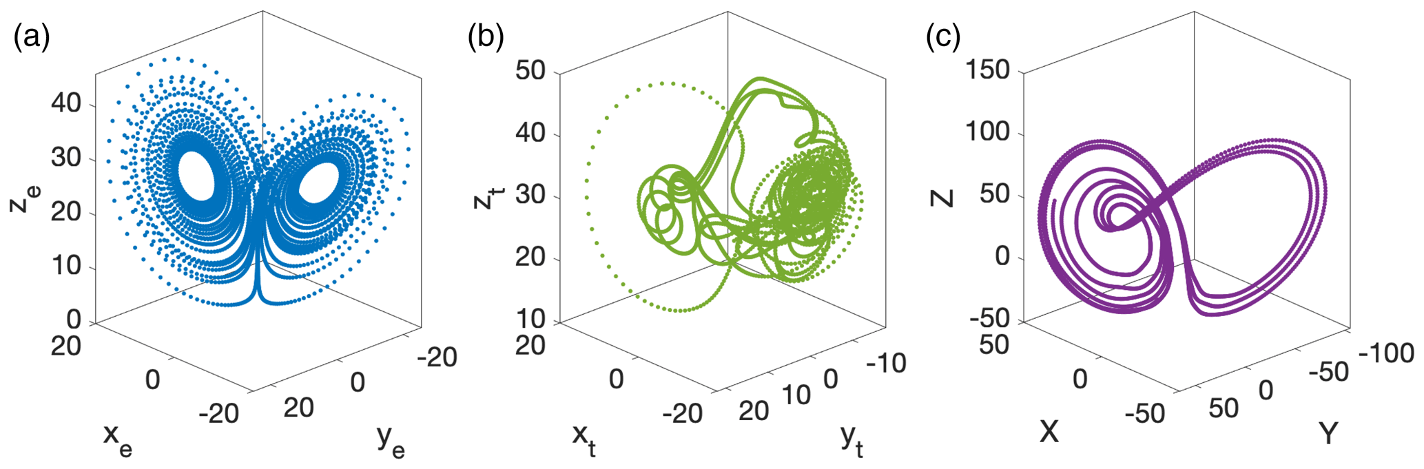
More generally, these choices lead to a tropical subsystem that is dominated by changes in the ocean subsystem, but has an extratropical atmosphere, representative of weather noise, whose behaviour is similar to the original Lorenz model in that the system exhibits chaotic behaviour with two distinct regimes observed in the x_e and y_e coordinates of the extratropical atmosphere. The ocean exhibits significant deviations from its normal trajectory about every 2–8 years, where 3 years corresponds to approximately 10 time units. Figure 1 shows typical trajectories of the x_e, x_t, and X components of the extratropical, tropical, and ocean subsystems respectively. Figure 2 shows the approximate phase space structure of each of the respective subsystem's attractors.

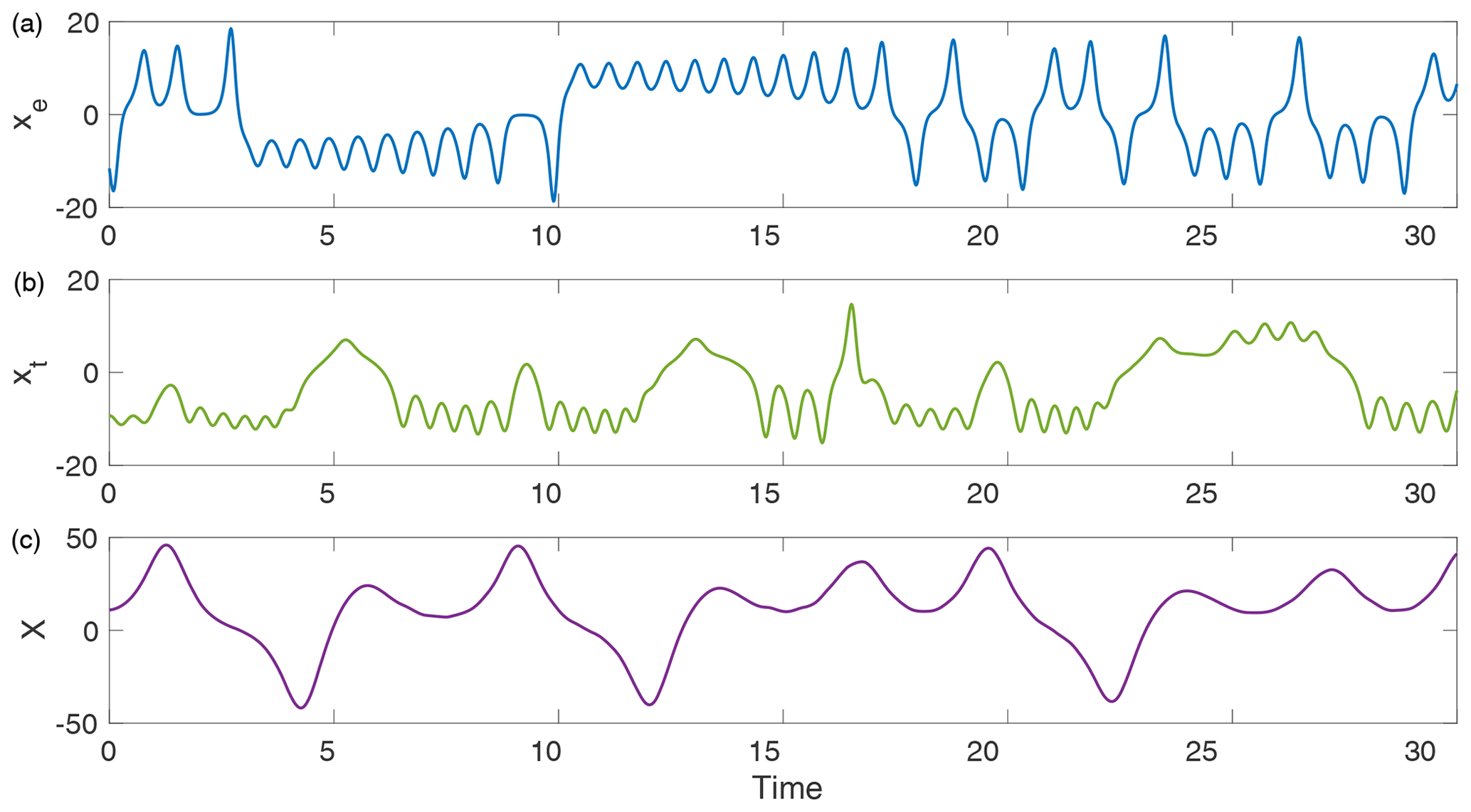
Figure 1 Example trajectories of the coupled Lorenz model (Eq. 1) for x_e (a), x_t (b), and X (c).

Figure 2 Trajectories along attractors of the extratropical (a), tropical (b), and ocean (c) subsystems of Eq. (1).

2.2 Lyapunov exponents and dimension

We are interested in analysing both the short-term and asymptotic dynamics of the system (1). We start by considering the asymptotic behaviour of trajectories, which can be understood through the Lyapunov exponents. Chaotic systems are characterized by one or more positive Lyapunov exponents (Benettin et al., 1976; Sano and Sawada, 1985), and the underlying attractor dimension can be related to the values of the Lyapunov exponents (Young, 1982; Eckmann and Ruelle, 1985).

Figure 3 (a) Convergence of Lyapunov exponents of Eq. (1) with an inset of zoom around zero to show the two neutral exponents. (b) Asymptotic values of Lyapunov exponents of Eq. (1).

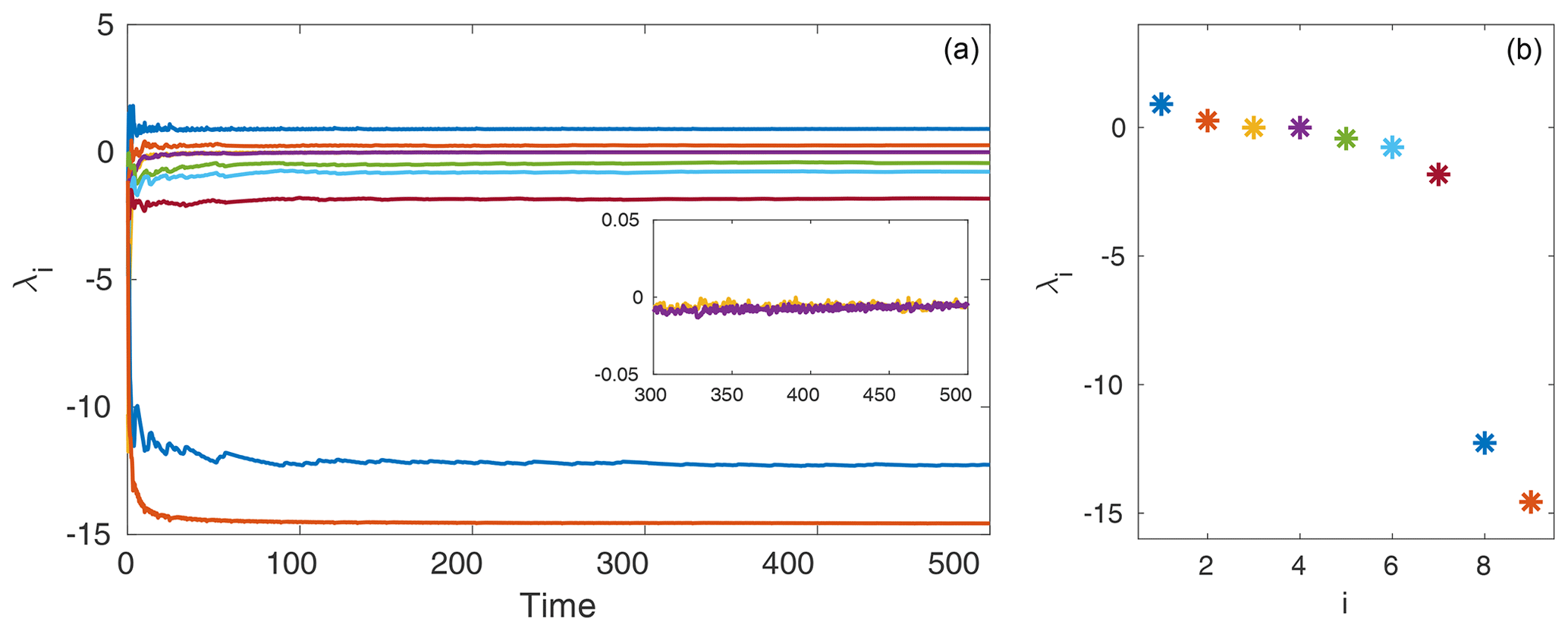
We compute the Lyapunov exponents using a QR decomposition method (see e.g. Dieci et al., 1997). For the computation we run the model for 1000 time units to ensure convergence onto the attractor. We use a time step of 0.01 and compute the Lyapunov exponents from the last 500 time units, with an orthonormalization time step of 0.25 for the QR method. The convergence of the Lyapunov exponents is shown in Fig. 3. We observe that for these parameter values there are two unstable and two approximately neutral Lyapunov exponents. We list the values of all nine computed asymptotic exponents in Table 1.

Table 1 Asymptotic Lyapunov exponents of Eq. (1) computed over 500 time units using a QR decomposition method, time step of 0.01, and orthogonalization step of 0.25.

Given the approximated asymptotic Lyapunov exponents in Table 1, we can compute the global attractor dimension, i.e. the number of active degrees of freedom. Note that there is a large spectral gap between the seventh and eighth Lyapunov exponents. This gives evidence that the effective dimension of the attractor will be less than eight. Throughout this study we will use the Kaplan–Yorke dimension (Kaplan and Yorke, 1979; Frederickson et al., 1983) to calculate the upper bound on the attractor dimension. It is defined as follows:

$$\begin{array}{}\text{(2)}& {\dim }_{\mathrm{KY}}:=j+{\displaystyle \frac{{\sum }_{i=\mathrm{1}}^j{\mathit{\lambda }}_i}{\left|{\mathit{\lambda }}_{j+\mathrm{1}}\right|}},\end{array}$$

where j is the largest integer such that $\sum _{i=\mathrm{1}}^j{\mathit{\lambda }}_i\ge \mathrm{0}$ and $\sum _{i=\mathrm{1}}^{j+\mathrm{1}}{\mathit{\lambda }}_i<\mathrm{0}$. In addition we calculate the Kolmogorov–Sinai entropy ent_KS as a measure of the diversity of the trajectories generated by the dynamical system and determined through the Pesin formula:

$$\begin{array}{}\text{(3)}& {\mathrm{ent}}_{\mathrm{KS}}=\sum _{\mathit{\lambda }>\mathrm{0}}{\mathit{\lambda }}_i,\end{array}$$

which provides an upper bound to the entropy (Eckmann and Ruelle, 1985).

With the values in Table 1 we obtain a value of 5.9473 for the global attractor dimension of the nine-component system. As previously mentioned, asymptotically stable modes can experience transient periods of linear unstable growth. We therefore define local dimension through the computation of Eq. (2) using finite-time Lyapunov exponents (FTLEs). The computation of FTLEs is similar to that of the asymptotic Lyapunov exponents, with the difference being a finite window of time over which the exponents are computed. The FTLEs then serve as a time-dependent measure of the local unstable, neutral, and stable growth rates of the evolving system (Abarbanel et al., 1991; Eckhardt and Yao, 1993; Yoden and Nomura, 1993). The temporal variability of FTLEs is highly dependent on the window size, τ, over which they are computed. As τ→∞ the variability reduces and the FTLEs approach the asymptotic Lyapunov exponent values (Yoden and Nomura, 1993). We compute the FTLEs for a window size τ=4 and the corresponding time-varying Kaplan–Yorke dimension which we will refer to as a “local” dimension. This will give a measure which reflects variations in the finite-time growth rates, with higher (lower) dimension signifying increased instability (stability) in the FTLEs. More specifically this is an upper bound on the true local dimension – the measure does not take into account the geometric degeneracy which can occur when many of the leading CLVs can become aligned. In practice this overestimation of dimension is actually beneficial within the DA framework (more discussion on this can be found in Sect. 4.2).

Figure 4 shows the local dimension plotted along the attractors of each of the subsystems. We see that the local dimension is lowest when the model is in the interior region of the ocean subsystem attractor. In contrast, the extratropical atmosphere subsystem attractor displays periods of low dimension largely uniformly confined to the centre of each lobe of the attractor. The tropical atmosphere also shows most of the measures of low dimension confined to the interior of the attractor, reflecting the strong ocean coupling.

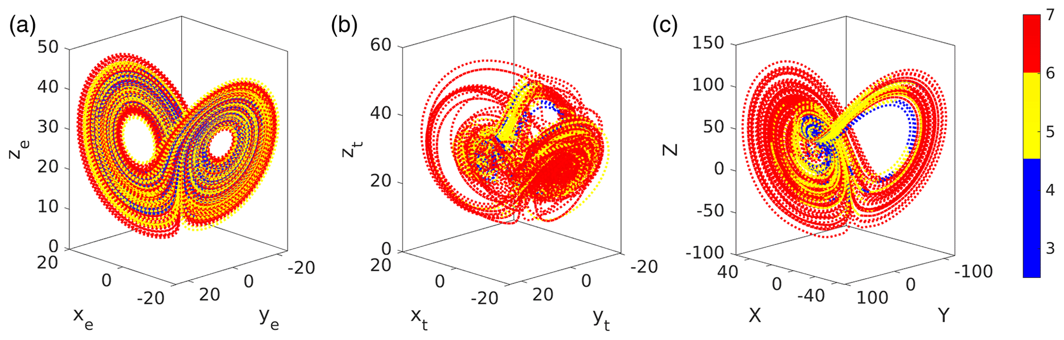
Figure 4 Local Kaplan–Yorke dimension plotted along the trajectory in phase space for the extratropical atmosphere (a), tropical atmosphere (b), and ocean (c) subsystems.

3 Covariant Lyapunov vectors

The existence of Lyapunov vectors for a large class of dynamical systems was proven by Oseledets (1968). The multiplicative ergodic theorem states that there exists a relation between Lyapunov exponents, λ_i, and a (non-unique) set of vectors ϕ such that

$$\begin{array}{}\text{(4)}& \begin{array}{rl}{\mathit{\lambda }}_i& =\underset{\mathit{\tau }\to \mathrm{\infty }}{lim}{\displaystyle \frac{\mathrm{1}}{\mathit{\tau }}}\log \left|\right|\mathcal{A}\left(x\right(t),\mathit{\tau })\mathit{\varphi }\left|\right|\mathrm{iff}\\ & \mathit{\varphi }\in {\mathrm{\Phi }}_i\left(x\right(t\left)\right)\setminus {\mathrm{\Phi }}_{i+\mathrm{1}}\left(x\right(t\left)\right).\end{array}\end{array}$$

Here, 𝒜(x(t),τ) is the forward and backward mapping of solutions under the tangent dynamics of a given dynamical system (also referred to as the cocycle). For system (1), $\mathcal{A}\left(x\right(t),\mathit{\tau })={\mathrm{e}}^{\mathit{\tau }Jf\left(x\right(t\left)\right)}$, where Jf denotes the Jacobian of f, the right-hand side of system (1). The subspaces (Φ_i) on which the growth rates (λ_i) occur are covariant with the tangent dynamics and invariant under time reversal (Ginelli et al., 2007; Froyland et al., 2013). The covariant Lyapunov vectors (CLVs) are then defined as the set of directions at each point in phase space that satisfy Eq. (4) both backwards and forwards in time (Ginelli et al., 2007; Ng et al., 2011). In the last few decades there have been significant advances in the ability to numerically approximate such vectors for chaotic dynamical systems (Ginelli et al., 2007; Wolfe and Samelson, 2007; Froyland et al., 2013). In this work we will employ a numerical algorithm introduced by Froyland et al. (2013) (Algorithm 2.2 in the aforementioned study). We summarize this algorithm below.

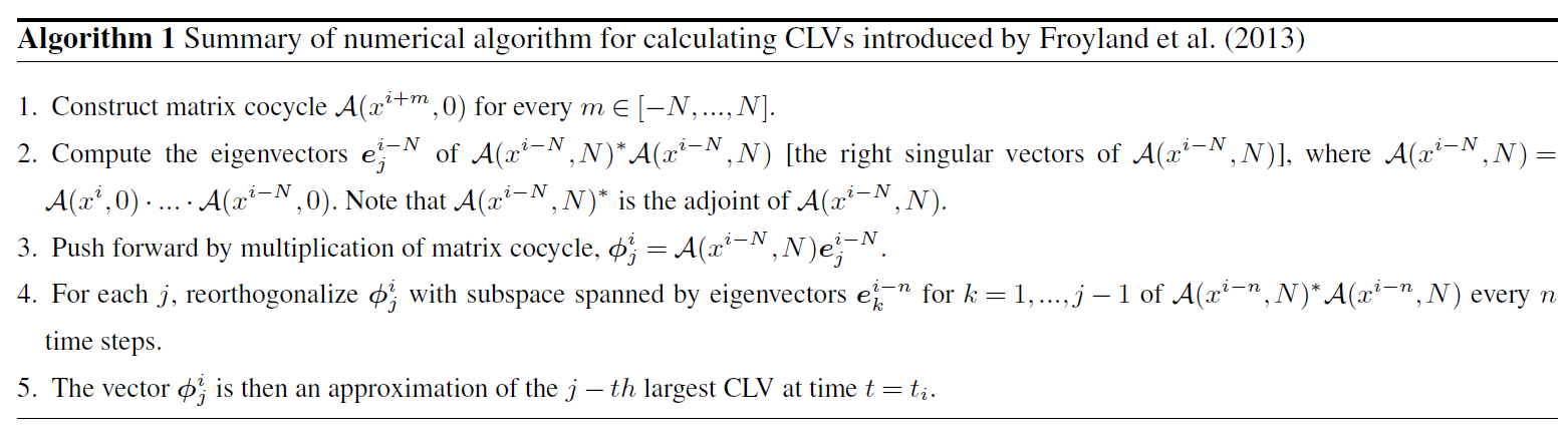
It should be mentioned that the push forward step need not be equal to N; M≠N for $\mathcal{A}(x^{i-N},M)$. However, for all calculations in this study we consider only the case M=N. The trajectory of the system is discretized with time step Δt such that xⁱ=x(t_i) and $x^{i+m}=x(t_i+m\mathrm{\Delta }t)$.

We examine the effectiveness of this algorithm on the Peña and Kalnay (2004) model introduced in Sect. 2. By definition, CLVs describe the directions in phase space corresponding to different growth rates. Two or more CLVs can align during a transition to a different regime in phase space. We calculate the alignment through

$$\begin{array}{}\text{(5)}& {\mathit{\theta }}_{i,j}={\displaystyle \frac{|{\mathit{\varphi }}_i\cdot {\mathit{\varphi }}_j|}{\left|\right|{\mathit{\varphi }}_i\left|\right|\cdot \left|\right|{\mathit{\varphi }}_j\left|\right|}}.\end{array}$$

Here, ${\mathit{\theta }}_{i,j}=\left|\cos \right({\mathrm{\Theta }}_{i,j}\left)\right|$, where Θ_i,j is the angle between the ith and jth CLVs. Larger values of θ_i,j imply alignment of the two CLVs. Figure 5 shows the alignment of the unstable CLVs (θ_1,2) and the neutral CLVs (θ_3,4) plotted against the X component of the system (1), along with the FTLEs and corresponding local time-varying Kaplan–Yorke dimension. Since the window to calculate the FTLEs was chosen based on the variability timescales of the ocean subsystem, the subsequent local dimension measure should reflect areas of increased or decreased instability along the ocean attractor (Fig. 4). We also expect alignment of the CLVs during a transition in this subsystem. The CLVs analysed in Fig. 5 are calculated from the first 35 time units of the previous model run with a time step Δt=0.01. We start the calculation at t=5 to allow for initialization and a window size of τ=4. The parameters for the algorithm are set as N=400 and n=25. It can be seen that the algorithm detects near alignment of either the unstable or neutral CLVs during the transitions in the ocean subsystem. The transitions here are between the inner part of the attractor with smaller oscillation amplitudes and the outer, large-amplitude excursions. In general, the alignment is most prominent in the outer, large-amplitude part of the attractor. This follows the changes in local dimension, shown in the lower panel of Fig. 5c. Higher local dimension tends to accompany alignment of the unstable and neutral CLVs. This relates to the inability of the Kaplan–Yorke dimension measure to account for finite-time geometric degeneracy.

Figure 5 Local dynamical properties of a segment of an example model run. (a) Alignment of CLVs associated with the unstable and neutral subspaces plotted along the x coordinate of the ocean subsystem. Large orange stars indicate high alignment of unstable or neutral CLVs (${\mathit{\theta }}_{\mathrm{1},\mathrm{2}}>\mathrm{0.9}$ or ${\mathit{\theta }}_{\mathrm{3},\mathrm{4}}>\mathrm{0.9}$). (b) Time-varying FTLEs Λ_i(t) computed over window τ=4. (c) Local Kaplan–Yorke dimension calculated from FTLEs.

At this point we will comment on the non-trivial relationship between the CLVs and FTLEs calculated here. As discussed in Vannitsem and Lucarini (2016), there are three different types of FTLEs one can compute: backward (FTBLEs), forward (FTFLEs), and covariant (FTCLEs). Each type of FTLE gives the local growth rate of the corresponding Lyapunov vectors. Although all three converge to the asymptotic Lyapunov exponents as the computation window increases, the temporal variability for finite window size can be different depending on the model at hand. Vannitsem and Lucarini (2016) found that when calculating the growth rates of the CLVs, higher variability in the FTCLEs corresponding to neutral or near-zero modes occurred compared to the other two methods. This could have implications for the local Kaplan–Yorke dimension if one were to use the FTCLEs rather than the FTBLEs in the calculation. We remark here that the QR method produces backward Lyapunov vectors (BLVs) and their corresponding FTBLEs. We therefore compare the Kaplan–Yorke dimension as computed from FTCLEs and FTBLEs for the coupled Lorenz system (1) in Fig. 6. We see that for this model the dimension calculated from FTBLEs approximately bounds that calculated from FTCLEs. Since we will be using the local Kaplan–Yorke dimension as a lower bound within the framework of our experiments, the FTBLEs give a conservative estimate of dimension that is varying with our dynamics (see Sect. 4.2 for discussion of the implementation of dimension in our experiments).

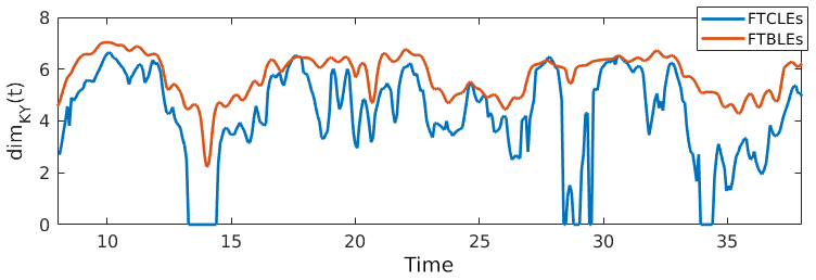
Figure 6 Comparison of the finite-time Kaplan–Yorke dimension calculated using the growth rates of CLVs (FTCLEs) and the QR method (FTBLEs).

In the following sections, we will utilize CLVs within the data assimilation framework of ensemble forecasting. The CLVs will be used to construct the forecast error covariance matrix, which informs the increment used on ensemble members to bring them closer to observations. Using CLVs in this context suggests a more accurate method of forming the forecast error covariance matrix when the true covariance is undersampled due to an insufficient number of ensemble members (see e.g. Palatella and Trevisan, 2015, where the authors applied a similar approach using BLVs on the classical Lorenz, 1963, and Lorenz, 1996, systems).

4 Data assimilation with the Kalman filter

We now summarize the Kalman filter equations. For detailed derivations we refer the interested reader to the reviews by Evensen (2003), Houtekamer and Zhang (2016), or Carrassi et al. (2018). Here we follow the notation of Carrassi et al. (2018). Consider a deterministic or stochastic model defined by

$$\begin{array}{}\text{(6)}& {\mathit{x}}_k={\mathcal{M}}_{k:k-\mathrm{1}}({\mathit{x}}_{k-\mathrm{1}},\mathit{p})+{\mathit{\eta }}_k,\end{array}$$

where x_k∈ℝ^N is the model state at time t=t_k, p∈ℝ^p are the model parameters, ${\mathcal{M}}_{k:k-\mathrm{1}}:{\mathbb{R}}^N\to {\mathbb{R}}^N$ is a function taking the model from time t_k−1 to t_k, and η_k is the model error at time t_k (for deterministic systems, let η_k=0). Suppose that there exists a time-dependent set of observations y∈ℝ^d which can be expressed as a function of the model state through

$$\begin{array}{}\text{(7)}& {\mathit{y}}_k={\mathcal{H}}_k\left({\mathit{x}}_k\right)+{\mathit{ϵ}}_k.\end{array}$$

The observation operator ${\mathcal{H}}_k:{\mathbb{R}}^N\to {\mathbb{R}}^d$ can be linear or nonlinear, and ϵ_k is the observational error.

In the Kalman filter method, Eqs. (6) and (7) are assumed to be linear, resulting in evolution and observation matrices ${\mathbf{M}}_{k:k-\mathrm{1}}$ and H_k respectively. The model and observation errors, η_k and ϵ_k, are taken to be uncorrelated in time (white noise) and from a Gaussian distribution with covariance matrices ${\mathbf{Q}}_k\in {\mathbb{R}}^{N\times N}$ and ${\mathbf{R}}_k\in {\mathbb{R}}^{d\times d}$ respectively. There are two basic steps to the Kalman filter method: forecast and analysis.

• Forecast equations

  $$\begin{array}{}\text{(8a)}& {\displaystyle }{\mathit{x}}_k^f& {\displaystyle }={\mathbf{M}}_{k:k-\mathrm{1}}{\mathit{x}}_{k-\mathrm{1}}^a,\text{(8b)}& {\displaystyle }{\mathbf{P}}_k^f& {\displaystyle }={\mathbf{M}}_{k:k-\mathrm{1}}{\mathbf{P}}_{k-\mathrm{1}}^a{\mathbf{M}}_{k:k-\mathrm{1}}^{\mathrm{T}}+{\mathbf{Q}}_k.\end{array}$$

• Analysis equations

  $$\begin{array}{}\text{(9a)}& {\displaystyle }{\mathbf{K}}_k& {\displaystyle }={\mathbf{P}}_k^f{\mathbf{H}}_k^{\mathrm{T}}[{\mathbf{H}}_k{\mathbf{P}}_k^f{\mathbf{H}}_k^{\mathrm{T}}+{\mathbf{R}}_k{]}^{-\mathrm{1}},\text{(9b)}& {\displaystyle }{\mathit{x}}_k^a& {\displaystyle }={\mathit{x}}_k^f+{\mathbf{K}}_k({\mathit{y}}_k-{\mathbf{H}}_k{\mathit{x}}_k^f),\text{(9c)}& {\displaystyle }{\mathbf{P}}_k^a& {\displaystyle }=({\mathbf{I}}_k-{\mathbf{K}}_k{\mathbf{H}}_k){\mathbf{P}}_k^{\mathrm{f}}.\end{array}$$

There is a difficulty in finding accurate solutions to Eqs. (8)–(9) for realistic systems which have high dimensions and are nonlinear (as is the case in weather and climate forecasting). Within the Kalman filter class, various ensemble filter variants have been applied to tracking trajectories in nonlinear systems. The most popular are the deterministic filters (Tippett et al., 2003; Sakov and Oke, 2008; Sakov et al., 2012).

4.1 Ensemble Kalman filtering

Ensemble Kalman filtering methods use Monte Carlo sampling to form the approximate error statistics of a model. An ensemble of model states x^f∈ℝ^N with a finite number of ensemble members m produces an approximation to the true error covariance matrix as follows. The ensemble forecast anomaly matrix ${\mathbf{X}}^{\mathrm{f}}\in {\mathbb{R}}^{N\times m}$ is constructed with respect to the ensemble mean ${\stackrel{\mathrm{‾}}{\mathit{x}}}^f\in {\mathbb{R}}^N$:

$$\begin{array}{}\text{(10a)}& {\displaystyle }{\stackrel{\mathrm{‾}}{\mathit{x}}}^f& {\displaystyle }={\displaystyle \frac{\mathrm{1}}{m}}\sum _{n=\mathrm{1}}^m{\mathit{x}}_n^f,\text{(10b)}& {\displaystyle }{\mathbf{X}}^{\mathrm{f}}& {\displaystyle }\equiv {\displaystyle \frac{\mathrm{1}}{\sqrt{m-\mathrm{1}}}}[{\mathit{x}}_{\mathrm{1}}^f-{\stackrel{\mathrm{‾}}{\mathit{x}}}^f,\mathrm{\dots },{\mathit{x}}_m^f-{\stackrel{\mathrm{‾}}{\mathit{x}}}^f].\end{array}$$

Note that we have dropped the time subscript k; the subscripts used here refer to individual ensemble members. The forecast error covariance matrices P^f are then constructed through

$$\begin{array}{}\text{(11)}& {\mathbf{P}}^{\mathrm{f}}=\left({\mathbf{X}}^{\mathrm{f}}\right)({\mathbf{X}}^{\mathrm{f}}{)}^{\mathrm{T}}.\end{array}$$

To preserve the variance of the ensemble through the analysis step, square-root (deterministic) schemes for ensemble Kalman filtering are often used. One such scheme is the ensemble transform Kalman filter (ETKF) developed by Bishop et al. (2001) and then further adapted for large, spatiotemporally chaotic systems by Hunt et al. (2007). In such schemes, the observations do not need to be perturbed to preserve the analysis covariance in Eq. (9c). The main idea is that a transform matrix T can be used to adjust the ensemble analysis anomalies matrix,

$$\begin{array}{}\text{(12)}& {\mathbf{X}}^a\equiv {\displaystyle \frac{\mathrm{1}}{\sqrt{m-\mathrm{1}}}}[{\mathit{x}}_{\mathrm{1}}^a-{\stackrel{\mathrm{‾}}{\mathit{x}}}^a,\mathrm{\dots },{\mathit{x}}_m^a-{\stackrel{\mathrm{‾}}{\mathit{x}}}^a]={\mathbf{X}}^{\mathrm{f}}\mathbf{T},\end{array}$$

which ultimately forms the analysis error covariance matrix,

$$\begin{array}{}\text{(13)}& {\mathbf{P}}^a=\left({\mathbf{X}}^a\right)({\mathbf{X}}^a{)}^{\mathrm{T}}.\end{array}$$

This transform matrix T is recovered by calculating the ensemble perturbations in normalized observation space:

$$\begin{array}{}\text{(14)}& \mathbf{S}={\mathbf{R}}^{-\mathrm{1}/\mathrm{2}}{\mathbf{HX}}^{\mathrm{f}}.\end{array}$$

The transform matrix T is then defined as

$$\begin{array}{}\text{(15)}& \mathbf{T}=(\mathbf{I}+{\mathbf{S}}^{\mathrm{T}}\mathbf{S}{)}^{-\mathrm{1}/\mathrm{2}},\end{array}$$

where I is the m×m identity matrix. See Bishop et al. (2001) for the full derivation. This leads to the update of the ensemble mean and the individual ensemble members to their analysed state through the equations

$$\begin{array}{}\text{(16a)}& {\displaystyle }{\stackrel{\mathrm{‾}}{\mathit{x}}}^a& {\displaystyle }={\stackrel{\mathrm{‾}}{\mathit{x}}}^f+\mathbf{K}(\mathit{y}-\mathbf{H}{\stackrel{\mathrm{‾}}{\mathit{x}}}^f),\text{(16b)}& {\displaystyle }{\mathit{x}}_n^a& {\displaystyle }={\stackrel{\mathrm{‾}}{\mathit{x}}}^a+\left(\sqrt{m-\mathrm{1}}\right)[{\mathbf{X}}^{\mathrm{f}}\mathbf{T}{]}_{*,n}.\end{array}$$

Following Bishop et al. (2001) we define the Kalman gain K through Eq. (9a), and the subscript $*,n$ denotes taking the nth column of the matrix.

Another deterministic scheme for ensemble Kalman filtering which uses a left-multiplied transform matrix was shown by Tippett et al. (2003) to be equivalent to ETKF:

$$\begin{array}{}\text{(17a)}& {\displaystyle }{\mathbf{X}}^a& {\displaystyle }={\mathbf{TX}}^{\mathrm{f}},\text{(17b)}& {\displaystyle }\mathbf{T}& {\displaystyle }=(\mathbf{I}-\mathbf{KH}{)}^{\mathrm{1}/\mathrm{2}}.\end{array}$$

We will refer to this left-multiplied transform filter as the ensemble square-root filter (ESRF). The ensemble mean is updated through Eq. (16a) and the individual ensemble members are then updated through

$$\begin{array}{}\text{(18)}& {\mathit{x}}_n^a={\stackrel{\mathrm{‾}}{\mathit{x}}}^a+\left(\sqrt{m-\mathrm{1}}\right)[{\mathbf{TX}}^{\mathrm{f}}{]}_{*,n}.\end{array}$$

When using ensemble Kalman filtering methods like the ones introduced here, sampling errors can often occur. For nonlinear models in particular, there is a systematic underestimation of analysis error covariances which eventually leads to filter divergence (Anderson and Anderson, 1999; Bocquet et al., 2015; Raanes et al., 2019). This is commonly avoided through the use of inflation. In other words, after each analysis step the ensemble anomalies are inflated through

$$\begin{array}{}\text{(19)}& {\mathit{x}}_n^a={\stackrel{\mathrm{‾}}{\mathit{x}}}^a+\mathit{\lambda }({\mathit{x}}_n^a-{\stackrel{\mathrm{‾}}{\mathit{x}}}^a),\mathit{\lambda }>\mathrm{1},\end{array}$$

where $(\mathit{\lambda }-\mathrm{1})/\mathrm{100}$ is the percentage inflation. Grudzien et al. (2018b) recently showed that the need for inflation tuning could potentially be compensated by including the asymptotic stable modes which produce transient instabilities. The following section introduces one way to account for such transient instabilities through a projection of the forecast error covariance matrix onto a subset of CLVs.

4.2 Ensemble filtering in reduced subspace

Here we define the error covariance matrix P^f based on the directions of growth and decay of errors associated with different timescales at the given analysis time. Specifically, we construct P^f using the CLVs computed at each data assimilation time step where the number of CLVs is determined by the local attractor dimension dim_KY. This allows for the inclusion of unstable, neutral and stable directions dependent on the local dynamics of the system. This differs from past approaches where the subspace was determined in terms of the asymptotic Lyapunov exponents, and therefore the rank of the error covariance matrix was kept fixed (Trevisan and Uboldi, 2004; Carrassi et al., 2008; Trevisan and Palatella, 2011; Palatella and Trevisan, 2015).

To determine the number of CLVs required to form the basis for P^f, we use the time-dependent or local dim_KY rounded up to an integer value. To determine how to weight the individual CLVs, we deconstruct the ensemble anomalies matrix defined in Eq. (10b), X^f, into

$$\begin{array}{}\text{(20)}& {\mathbf{X}}^{\mathrm{f}}=\mathbf{\Phi }\mathbf{W},\end{array}$$

where Φ is a matrix with columns equal to the CLVs (ϕ_i) and W is a matrix of weights. The columns of Φ are ordered according to the corresponding FTLEs in descending order (the first being the direction corresponding to the fastest unstable growth). In this formulation Φ need not be square, i.e. the CLVs used do not need to span the entire space. We compute the CLVs at the assimilation step using Algorithm 1. Equation (20) can then be solved for W in a least-squares sense through

$$\begin{array}{}\text{(21)}& \mathbf{W}=({\mathbf{\Phi }}^{\mathrm{T}}\mathbf{\Phi }{)}^{-\mathrm{1}}{\mathbf{\Phi }}^{\mathrm{T}}{\mathbf{X}}^{\mathrm{f}}.\end{array}$$

The weights in W combined with the directions in Φ now define an object with dimension equal to the chosen number of CLVs whose covariance matrix is defined by

$$\begin{array}{}\text{(22)}& {\mathbf{P}}^{\mathrm{f}}=\mathbf{\Phi }{\mathbf{WW}}^{\mathrm{T}}{\mathbf{\Phi }}^{\mathrm{T}}.\end{array}$$

We can then use the formulation of P^f above in conjunction with the ensemble schemes of Sect. 4.1. We use the modified forecast covariance matrix (Eq. 22) in the calculation of the Kalman gain (Eq. 9a), which then also alters any subsequent calculations.

It is important that we span the local dimension of the attractor within the ensemble DA framework in order to avoid ensemble collapse. As mentioned in Sect. 3, the Kaplan–Yorke dimension computed from the FTLEs is an upper bound to the true local dimension. Figure 7 shows the alignment of the CLVs at two time instances of a model run where the leading FTLEs behave similarly and consequently the Kaplan–Yorke dimensions are approximately the same. In the first case (t=306.24), the leading five CLVs are strongly aligned as well as the two most stable (8 and 9). The dimension based on alignment would then intuitively be around four, and one would need to select the set of CLVs that are not aligned in order to avoid ensemble collapse. According to our method, since the local Kaplan–Yorke dimension is greater than seven, we would retain the leading eight CLVs, therefore retaining all necessary directions to maintain spread. The second case (t=705.04) shows very different alignment behaviour. Here the leading CLVs are not strongly aligned, but there is strong alignment of CLVs 4–6 and pairs 3, 7, 8, and 9. This would give an alignment-based dimension around five, but again we need to retain up to the eighth CLV to span the independent directions. While one could create a method based on alignment for selecting directions, we point out that the actual criterion for “strong alignment” is arbitrary, and one could risk excluding a significant direction. For this reason we argue that the local Kaplan–Yorke measure gives a conservative estimate for the number of CLVs to retain.

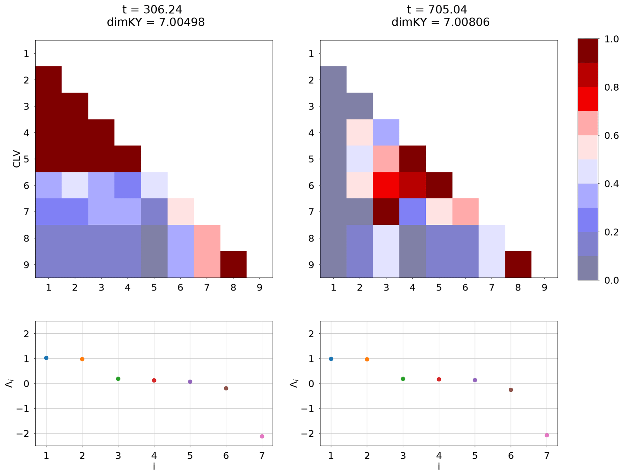
Figure 7 We compare the alignment of the CLVs at two time steps of a model run. The two time steps have a similar Kaplan–Yorke measure with the distribution of the leading FTLEs, shown in the bottom panels. We observe that the behaviour of the alignment can be vastly different for similar FTLE behaviour; however, the method of retaining CLVs based on the Kaplan–Yorke measure gives a reliable way of reflecting the true local dimension regardless of alignment.

5 Results

We perform a collection of data assimilation experiments for the system (1) using a control run as observations (computed using a Runga–Kutta fourth-order scheme with Δt=0.01). Here we emphasize that we are interested in exploring the dynamical attributes of data assimilation across multiple timescales. In all the cases we are using standard strong CDA, meaning that the cross-covariances are used amongst all components regardless of the observation set (Laloyaux et al., 2016; O'Kane et al., 2019). This allows for the analysis increment of any unobserved subsystems to be influenced by the observations, even in cases of weak coupling between the subsystems. We experiment with different observation sets to explore the applicability and performance of the variable-rank strong CDA with incomplete or temporally correlated observations. Such observation sets are arguably more realistic representations of the types of observations used in climate applications.

The initialization settings for the DA experiments are as follows, unless otherwise stated. We use the settings from Yoshida and Kalnay (2018): assimilation window 0.08, inflation factor 1 % (optimal for all experiments unless noted otherwise), and 10 ensemble members. We run the model for 75 000 time steps (9375 assimilation windows) and use 50 000 time steps (6250 assimilation windows) for calculating analysis error statistics. The model is allowed to spin up for 400 time steps before starting the assimilation cycles as we are using a window of τ=4 for the calculation of the FTLEs and CLVs. We note that for the CLV method, the system must be sufficiently tracking the control to accurately calculate the initial CLVs. For this reason we start the assimilation before there is significant ensemble divergence. The ensemble members are initialized as perturbations from the control initial condition, taken from a uniform distribution defined on $[-\mathrm{0.025},\mathrm{0.025}]$.

The dynamical properties of the experiments are calculated with respect to the ensemble mean trajectory. The FTLEs are computed using the QR decomposition over the previous 400 time steps leading up to the assimilation time step. The local Kaplan–Yorke dimension is then calculated from the FTLEs. The CLVs are then calculated using a slight modification to Algorithm 1 – due to the absence of an accurate future trajectory of the ensemble mean, we do not perform the reorthogonalization to the eigenvectors of $\mathcal{A}(x^{i-n},N{)}^{*}\mathcal{A}(x^{i-n},N)$ (step 4). This is equivalent to using Algorithm 2.1 of Froyland et al. (2013). We use the previous 400 time steps of the ensemble mean trajectory leading up to the assimilation time step to compute the matrix cocycle and subsequently the CLVs.

5.1 Constructing the observations

In the Kalman filtering method introduced in Sect. 4, there is an underlying assumption that the observations have some error with variance R. This error variance is typically unknown and chosen a priori. If we consider the observations in a statistical sense, we can deconstruct them at each assimilation step into a mean field and perturbation value: $\mathit{y}=\stackrel{\mathrm{‾}}{\mathit{y}}+\widehat{\mathit{y}}$. In such a formulation, $\stackrel{\mathrm{‾}}{\mathit{y}}$ would be the truth at a given point in time and the observation error variance would be the average of the variance of the perturbations, $\mathbf{R}=\stackrel{\mathrm{‾}}{\widehat{\mathit{y}}{\widehat{\mathit{y}}}^{\mathrm{T}}}$. To emulate this in deterministic models where the truth $\stackrel{\mathrm{‾}}{\mathit{y}}$ is known (i.e. from a control run), it is common practice to construct the observations by adding to the truth a random value $\widehat{\mathit{y}}$ taken from a normal distribution with variance given by the diagonals of R. However, this produces uncorrelated observation errors which have the same variance at any given point in phase space. In many applications the true variance of the observation error can be spatially dependent and errors are often correlated in time (O'Kane and Frederiksen, 2008). We therefore also consider the case where there is error in the observations, but it is consistent with the underlying nonlinear dynamics by constructing a trajectory that “shadows” the truth. Both types of observational errors, with the additional case of perfectly observing a subset of variables, are explored.

The main differences in our subsequent experiments are in the subset of observations used and their corresponding observational errors. We aim to assess the performance of the reduced-rank strong CDA within the different configurations. We first present a benchmark test on the CLV method which is identical to an experiment presented in Yoshida and Kalnay (2018), where the y component of each subsystem is observed. The perturbations to the control run are from a normal distribution with error variance $\mathbf{R}=\mathrm{diag}\left(\right[\mathrm{1},\mathrm{1},\mathrm{25}\left]\right)$. This case is referred to as benchmark observations. We then consider two experiments where the observations are less sparse within the subsystems; however, one subsystem is completely unobserved: atmosphere observations ($y_{\mathrm{e}},z_{\mathrm{e}},y_t,z_t$) and ENSO (El Niño–Southern Oscillation) observations ($y_t,z_t,Y,Z$). For the atmosphere observations case we sample the perturbations from error variance R=I₄, while for the ENSO observations we experiment with different error variances. We then consider correlated observation errors through shadowed observations. For these experiments the observation error variances R are set to the standard values from Yoshida and Kalnay (2018), but the actual perturbations are constructed through a model trajectory which is initialized close to the control run and forced by a relaxation term back to the control. The observation errors then also reflect the local nonlinear growth. We repeat the benchmark, atmosphere, and ENSO observation cases with this type of observation error. Finally, we reduce the observation space to only the extratropical subsystem ($x_{\mathrm{e}},y_{\mathrm{e}},z_{\mathrm{e}}$). This extends upon the work in O'Kane et al. (2019), where the authors considered only ocean observations (X, Y, Z). Due to the difficulty of constraining a system through only fast, weakly coupled dynamics, we decrease the assimilation window and assume perfect observations.

5.2 Benchmark observations

The first DA experiment we consider is a benchmark case with observations ($y_{\mathrm{e}},y_t,Y$). We reproduce the results in Yoshida and Kalnay (2018) using the CLV method introduced in Sect. 4.2. We first perform a DA experiment using a full-rank covariance matrix (equivalent to the ETKF method introduced in Sect. 4.1) and then compare it to using reduced subspace methods. The first reduced subspace method uses a fixed number of CLVs defined by spanning the asymptotic unstable and neutral subspace plus the first stable mode as in Ng et al. (2011). The second reduced subspace method also uses a fixed number of CLVs, except the number is defined by the asymptotic Kaplan–Yorke dimension as suggested in Carrassi et al. (2008) (note in that study that the authors discuss the number of ensemble members which is equivalent to the rank of the covariance matrix). These fixed numbers are five and six CLVs respectively. Finally we analyse our novel reduced subspace method which uses a variable number of CLVs based on the local Kaplan–Yorke dimension. We note that all experiments perform similarly when using the BLVs instead of the CLVs; however, BLVs do not provide the same local phase-space information. While we focus on the performance of the CLV method in this work, we include a comparison using BLVs for the experiment utilizing local dimension.

The error statistics of all the experiments are listed in Table 2. The analysis RMSE is calculated for each subsystem individually at every assimilation step and then averaged over the steps, in line with the error statistics produced in Yoshida and Kalnay (2018). We also calculate the average RMSE of the full system. The RMSE is defined as

$$\begin{array}{}\text{(23)}& \mathrm{RMSE}=\sqrt{{\displaystyle \frac{\mathrm{1}}{N}}({\stackrel{\mathrm{‾}}{\mathit{x}}}^a-\mathit{x}{)}^{\mathrm{T}}({\stackrel{\mathrm{‾}}{\mathit{x}}}^a-\mathit{x})},\end{array}$$

where N is the number of states in the analysed system (either 3 or 9) and x is the truth (control run in our case). We also calculate the spread and average increment for each state variable through

$$\begin{array}{}\text{(24)}& \begin{array}{rl}& \mathrm{spread}=\sqrt{\mathrm{diag}\left({\mathbf{P}}^{\mathrm{f}}\right)},\\ & \mathrm{average}\mathrm{increment}=\stackrel{\mathrm{‾}}{({\mathit{x}}^a-{\mathit{x}}^f)}.\end{array}\end{array}$$

Finally, we calculate the bias with respect to our observations y:

$$\begin{array}{}\text{(25)}& \mathrm{bias}=\stackrel{\mathrm{‾}}{(\mathit{y}-\mathbf{H}{\mathit{x}}^f)}.\end{array}$$

Table 2 Summary metrics of DA experiments using a right-transform matrix (Eq. 15) and benchmark observations ($y_{\mathrm{e}},y_t,Y$). The angle brackets 〈⋅〉 denote the average over assimilation steps. Compare to results in Yoshida and Kalnay (2018). Parameters: assimilation window 0.08, inflation factor 1 %, 10 ensemble members.

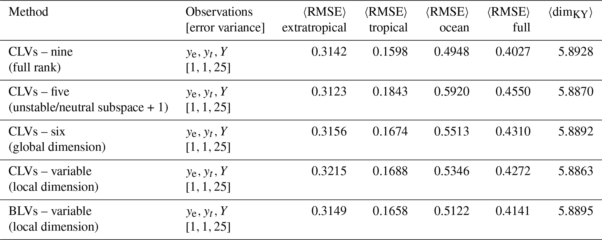
We observe that all experiments generally succeed at constraining the full system. The trajectories, spread, increments, and error metrics of the variable CLV experiments are shown in Fig. 8; all other experiments behave qualitatively similarly. When comparing the reduced subspace experiments to the full-rank case in Table 2, we find that using five CLVs (unstable, neutral, and one stable) performs worse than the other CLV experiments. While using the asymptotic Kaplan–Yorke dimension (six CLVs) shows improvement over five CLVs, the most improvement is in the variable CLV (and BLV) case. Although all the methods produce a comparable average dimension (last column of Table 2), our experiments show that taking into account local variations in dimension is most effective.

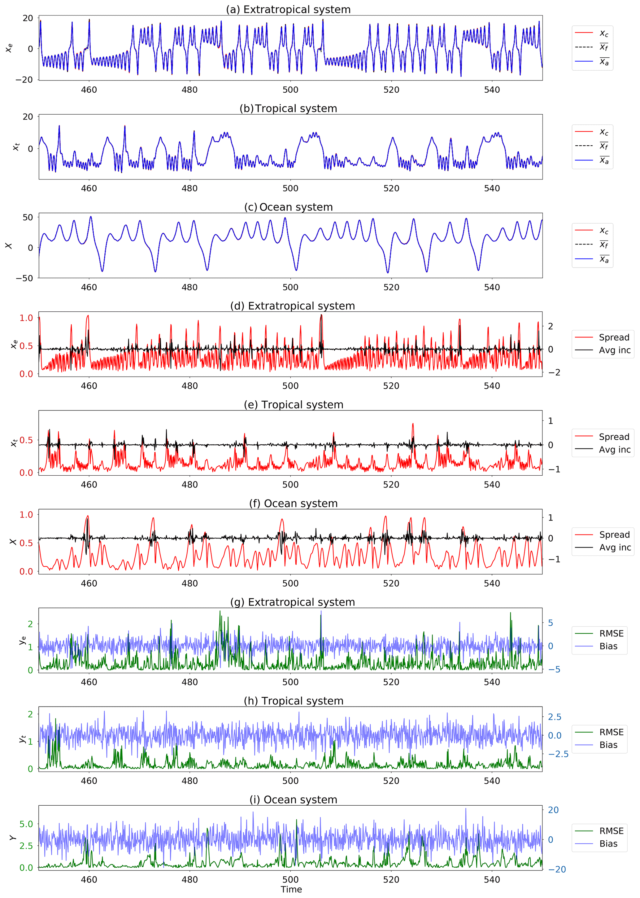
Figure 8 Segment of DA using the variable CLV method and benchmark observations ($y_{\mathrm{e}},y_t,Y$). (a–c) Trajectories shown are control run (red), ensemble mean (blue), and individual ensemble members (faint). (d–f) Metrics shown are the size of the ensemble spread (red) and ensemble mean increment (black). (g–i) Metrics shown are root mean square error (RMSE, green) and bias (blue). For conciseness we only show the results for one coordinate of each subsystem. The other two coordinates behave similarly. Parameters: assimilation window 0.08, inflation factor 1 %, 10 ensemble members, and observation error covariance matrix $\mathbf{R}=\mathrm{diag}\left(\right[\mathrm{1},\mathrm{1},\mathrm{25}\left]\right)$.

To take a closer inspection of the dynamics during the assimilation, Fig. 9 shows the corresponding dynamical properties of the variable CLV experiment in time. Panel (a) shows the FTLEs computed from the ensemble mean. The first thing to note is the correlation of the temporal FTLE variations. The most unstable and most stable modes have the same frequency of variability and remain highly correlated throughout the whole experiment. The lower-frequency variations seen in the second most stable mode are often correlated with some of the weakly stable modes. These seem to have the biggest impact on the local dimension (shown in panel b). We can compare the changes in FTLEs and local dimension to the rank of the covariance matrix (panel c). A decrease in local dimension typically occurs when one of the weakly stable modes becomes more stable, and therefore fewer CLVs are needed to span the local unstable and neutral subspace. In contrast, when the dimension increases, the weakly stable modes become more unstable, at times even becoming positive. This implies that more CLVs are needed to span the local unstable and neutral subspace, and therefore the rank of the covariance matrix increases. The local Kolmogorov–Sinai entropy is also shown with the local dimension. We see that directly before a full-dimension collapse (dim_KY=0), there is a spike in local entropy. A collapse in dimension here occurs when all the FTLEs become negative. This does not impact the effectiveness of the method, however, as it just enforces the covariance matrix and Kalman gain to be zero for that analysis step. The ensemble members are not adjusted and are therefore left to evolve accordingly. Figure 9d shows the statistics of the FTLEs. The mean values, shown as a full circle, are used to calculate the average dimension in Table 2. These can be compared to the asymptotic values computed in Sect. 2.2 which are shown as open circles to the right of the FTLE statistics. We also show the standard deviation for each of the FTLEs. The largest standard deviations are found in the fifth and sixth FTLEs, which correspond to the first two stable modes of the system. This supports the hypothesis that the weakly stable modes are most influential in the variation of local dimension. We also see that the maximum values are greater than (or equal to) zero. This implies that at a given time the fifth and sixth modes have moved into the unstable/neutral subspace and additional modes are therefore needed to account for nonlinear error growth.

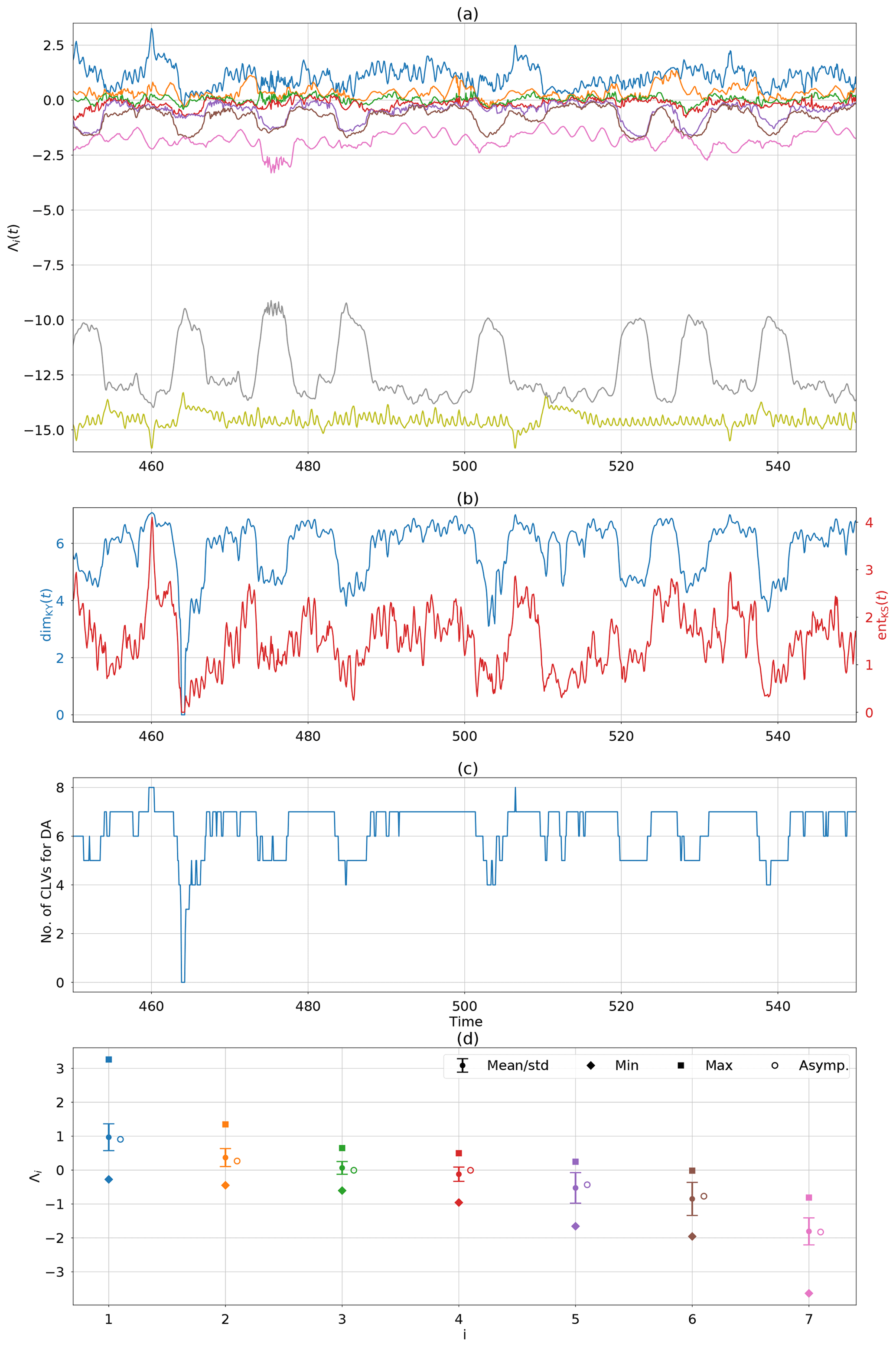
Figure 9 Local attractor properties of DA using the variable CLV method and benchmark observations ($y_{\mathrm{e}},y_t,Y$). (a) FTLEs calculated from the ensemble mean trajectory over a window of τ=4. (b) Local Kaplan–Yorke dimension and Kolmogorov–Sinai entropy computed through Eqs. (2) and (3) using the FTLEs at the given time. (c) Rank of the covariance matrix. (d) Statistics of the first seven FTLEs compared to asymptotic values.

5.3 Atmosphere observations

We now consider the case where only the two atmosphere subsystems are observed; however, the observations are less sparse within each subsystem in that we take both the y and z components. Yoshida and Kalnay (2018) considered a similar case where only y component observations were used with the cross-covariances in the atmosphere, but the ocean was also observed and assimilated separately. Here we rely only on the cross-covariances to recover the ocean subsystem, as the ocean is strongly coupled to the tropical atmosphere. For this case we use the following settings: assimilation window 0.08, observation error covariance matrix R=I₄, inflation factor 1 %, and 10 ensemble members. The model is run for the same amount of time as in the benchmark observation experiments.

Table 3 Summary metrics of DA experiments using a right-transform matrix (Eq. 15) and atmosphere observations ($y_{\mathrm{e}},z_{\mathrm{e}},y_t,z_t$). Parameters: assimilation window 0.08, inflation factor 1 %, 10 ensemble members.

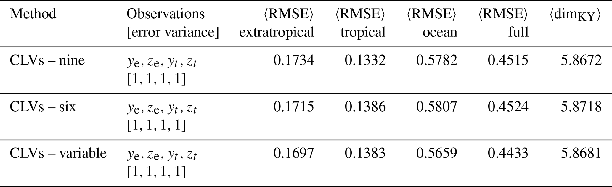
Table 3 shows the summary statistics of performing full-rank DA (nine CLVs), rank equal to the number of CLVs corresponding to asymptotic dimension, and a variable rank equal to the number of CLVs corresponding to local dimension. All the experiments have comparable summary statistics; however, the variable CLV experiment slightly outperforms both fixed-rank methods (Table 3). We also analysed the dynamical properties of the variable CLV experiment and did not find any significant differences to those of the benchmark experiment (Fig. 9).

5.4 ENSO observations

The strong coupling and low-frequency variation in the ocean and tropical atmosphere subsystems represent an ENSO-like variability. We therefore refer to the case of observing the y and z components from the tropical and ocean subsystems as ENSO observations. Again, this is similar to a case studied in Yoshida and Kalnay (2018), except that we do not assimilate the extratropical atmosphere at all and attempt to recover the variability solely through the cross-covariances. We do not expect to track the control trajectory of the extratropical system, but we are interested to see whether we can avoid collapse (i.e. the loss of variability) in the ensemble mean of the extratropical attractor.

Since the extratropical subsystem is likely to be unconstrained with these observations, the ensemble mean will not be accurately estimated. In such a case, the variable CLV method fails due to the fact that the first CLV (which corresponds to the directions of fastest error growth) is inaccurately calculated. Therefore the true directions of unstable growth are inaccurately sampled in the reduced space experiments. This is amplified by the fact that we are using uncorrelated observation errors; if the observation errors have a temporal correlation, the dominant direction of nonlinear unstable growth can be ascertained even without tracking the extratropical subsystem (see the following section on shadowed observations). The inaccurate dimension reduction leads to exponential growth in the system and numerical instability. For this reason we turn our focus only on the full-rank (nine CLVs) method and the accuracy of the observations.

We use the following settings for all the DA experiments with ENSO observations: assimilation window 0.08, inflation factor 1 %, and 10 ensemble members. The model is run for the same amount of time as in the benchmark observation experiments. We study the effect of reducing the observation error variances in R: standard observation error ($\mathbf{R}=\mathrm{diag}\left(\right[\mathrm{1},\mathrm{1},\mathrm{25},\mathrm{25}\left]\right)$), reduced tropical atmosphere error ($\mathbf{R}=\mathrm{diag}\left(\right[\mathrm{0.01},\mathrm{0.01},\mathrm{25},\mathrm{25}\left]\right)$), reduced ocean error ($\mathbf{R}=\mathrm{diag}\left(\right[\mathrm{1},\mathrm{1},\mathrm{0.25},\mathrm{0.25}\left]\right)$), and reduced overall error ($\mathbf{R}=\mathrm{diag}\left(\right[\mathrm{0.01},\mathrm{0.01},\mathrm{0.25},\mathrm{0.25}\left]\right)$). The summary statistics are listed in Table 4 for all the experiments.

Table 4 Summary metrics of DA experiments using right-transform matrix (15) and ENSO observations ($y_t,z_t,Y,Z$). Parameters: assimilation window 0.08, inflation factor 1 %, 10 ensemble members.

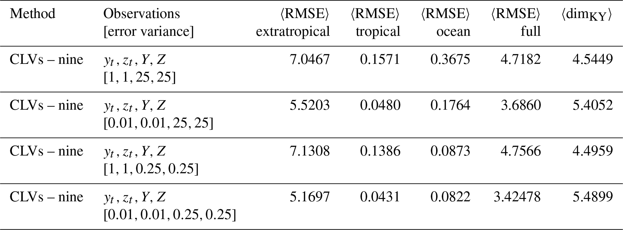
We find that for the standard observation errors, there is a collapse in the variance of the ensemble mean for the extratropical subsystem (Fig. 10). However, when the observation error for the tropical subsystem is reduced, that variance is significantly increased. This can be seen through the increase in the average local Kaplan–Yorke dimension (Table 4). There is also a slight increase in the ability to track the extratropical subsystem of the control run. We note that decreasing the ocean observation error alone does not provide any improvements over the total error statistics or dimension, actually making them slightly worse. When the observation error of both subsystems is reduced, there is only a small improvement to the overall error statistics and dimension in comparison to the reduced tropical error case. The improvement is most notable for the cases with reduced tropical observation errors due to the tropical system's weak direct coupling to the extratropical system.

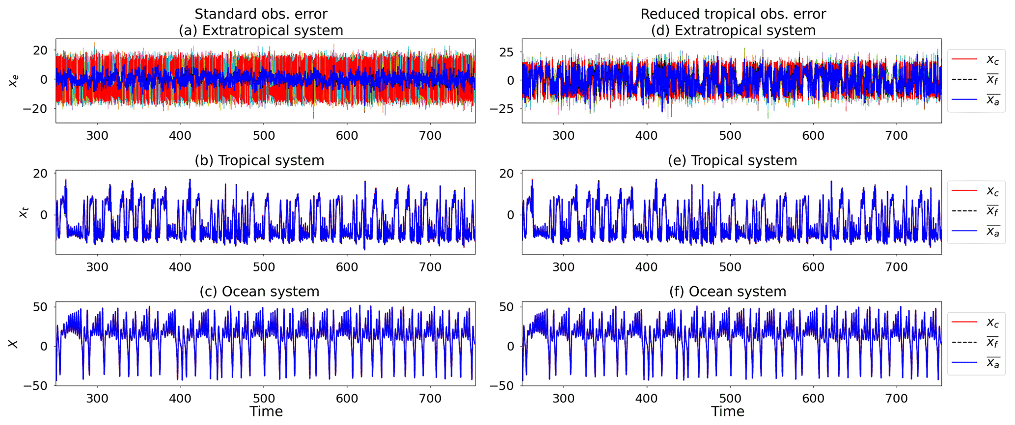
Figure 10 Trajectories of DA using nine CLVs, $\mathbf{R}=\mathrm{diag}\left(\right[\mathrm{1},\mathrm{1},\mathrm{25},\mathrm{25}\left]\right)$ (a–c), and $\mathbf{R}=\mathrm{diag}\left(\right[\mathrm{0.01},\mathrm{0.01},\mathrm{25},\mathrm{25}\left]\right)$ (d–f) with ENSO observations ($y_t,z_t,Y,Z$). Trajectories shown are control run (red), ensemble mean (blue), and individual ensemble members (multicoloured). For conciseness we only show the results for the x coordinate of each subsystem. The other two coordinates behave similarly. Parameters: assimilation window 0.08, inflation factor 1 %, 10 ensemble members.

5.5 Shadowed observations

In this section we explore a different type of observation error. Rather than randomly perturbing the control run to form our observation points, we use a trajectory that shadows the control run which produces correlated observational errors. In other words, we construct a new trajectory with a relaxation to the control run. This is implemented in the model as follows:

$$\begin{array}{ll}\text{(26a)}& {\displaystyle }{\dot{\stackrel{\mathrm{̃}}{x}}}_{\mathrm{e}}& {\displaystyle }=\mathit{\sigma }({\stackrel{\mathrm{̃}}{y}}_{\mathrm{e}}-{\stackrel{\mathrm{̃}}{x}}_{\mathrm{e}})-c_e(S{\stackrel{\mathrm{̃}}{x}}_t+k_{\mathrm{1}}),\text{(26b)}& {\displaystyle }{\dot{\stackrel{\mathrm{̃}}{y}}}_{\mathrm{e}}& {\displaystyle }=\mathit{\rho }{\stackrel{\mathrm{̃}}{x}}_{\mathrm{e}}-{\stackrel{\mathrm{̃}}{y}}_{\mathrm{e}}-{\stackrel{\mathrm{̃}}{x}}_{\mathrm{e}}{\stackrel{\mathrm{̃}}{z}}_{\mathrm{e}}+c_e(S{\stackrel{\mathrm{̃}}{y}}_t+k_{\mathrm{1}})+{\mathit{\alpha }}_{\mathrm{1}}(y_{\mathrm{e}}-{\stackrel{\mathrm{̃}}{y}}_{\mathrm{e}}),\text{(26c)}& {\displaystyle }{\dot{\stackrel{\mathrm{̃}}{z}}}_{\mathrm{e}}& {\displaystyle }={\stackrel{\mathrm{̃}}{x}}_{\mathrm{e}}{\stackrel{\mathrm{̃}}{y}}_{\mathrm{e}}-\mathit{\beta }{\stackrel{\mathrm{̃}}{z}}_{\mathrm{e}},\text{(26d)}& {\displaystyle }{\dot{\stackrel{\mathrm{̃}}{x}}}_t& {\displaystyle }=\mathit{\sigma }({\stackrel{\mathrm{̃}}{y}}_t-{\stackrel{\mathrm{̃}}{x}}_t)-c(S\stackrel{\mathrm{̃}}{X}+k_{\mathrm{2}})-c_e(S{\stackrel{\mathrm{̃}}{x}}_{\mathrm{e}}+k_{\mathrm{1}}),\text{(26e)}& {\displaystyle }{\dot{\stackrel{\mathrm{̃}}{y}}}_t& {\displaystyle }=\mathit{\rho }{\stackrel{\mathrm{̃}}{x}}_t-{\stackrel{\mathrm{̃}}{y}}_t-{\stackrel{\mathrm{̃}}{x}}_t{\stackrel{\mathrm{̃}}{z}}_t+c(S\stackrel{\mathrm{̃}}{Y}+k_{\mathrm{2}})+c_e(S{\stackrel{\mathrm{̃}}{y}}_{\mathrm{e}}+k_{\mathrm{1}}){\displaystyle }& {\displaystyle }+{\mathit{\alpha }}_{\mathrm{2}}(y_t-{\stackrel{\mathrm{̃}}{y}}_t),\\ \text{(26f)}& {\displaystyle }{\dot{\stackrel{\mathrm{̃}}{z}}}_t& {\displaystyle }={\stackrel{\mathrm{̃}}{x}}_t{\stackrel{\mathrm{̃}}{y}}_t-\mathit{\beta }{\stackrel{\mathrm{̃}}{z}}_t+c_z\stackrel{\mathrm{̃}}{Z},\text{(26g)}& {\displaystyle }\dot{\stackrel{\mathrm{̃}}{X}}& {\displaystyle }=\mathit{\tau }\mathit{\sigma }(\stackrel{\mathrm{̃}}{Y}-\stackrel{\mathrm{̃}}{X})-c({\stackrel{\mathrm{̃}}{x}}_t+k_{\mathrm{2}}),\text{(26h)}& {\displaystyle }\dot{\stackrel{\mathrm{̃}}{Y}}& {\displaystyle }=\mathit{\tau }\mathit{\rho }\stackrel{\mathrm{̃}}{X}-\mathit{\tau }\stackrel{\mathrm{̃}}{Y}-\mathit{\tau }S\stackrel{\mathrm{̃}}{X}\stackrel{\mathrm{̃}}{Z}+c({\stackrel{\mathrm{̃}}{y}}_t+k_{\mathrm{2}})+{\mathit{\alpha }}_{\mathrm{3}}(Y-\stackrel{\mathrm{̃}}{Y}),\text{(26i)}& {\displaystyle }\dot{\stackrel{\mathrm{̃}}{Z}}& {\displaystyle }=\mathit{\tau }S\stackrel{\mathrm{̃}}{X}\stackrel{\mathrm{̃}}{Y}-\mathit{\tau }\mathit{\beta }\stackrel{\mathrm{̃}}{Z}-c_z{\stackrel{\mathrm{̃}}{z}}_t.\end{array}$$

It is sufficient to constrain the trajectory using the relaxation term only in the y coordinates. The parameters α₁=2.75, α₂=0.8, and α₃=0.8 are the relaxation strengths and y_e(t), y_t(t), and Y(t) are taken from the control trajectory at the given time.

We initialize the shadowed trajectory with a small perturbation to the control trajectory initial condition. We then propagate the shadowed trajectory along with the control trajectory, taking the observations from the shadowed trajectory at each assimilation cycle. Figure 11 shows the difference between the observations constructed using random perturbations and those from the shadowed trajectory. One benefit of the shadowed trajectory which is clearly visible in these figures is that it much more closely maintains the structure of the attractor. This is not the case when using randomized perturbations, where the structure is not as discernible.

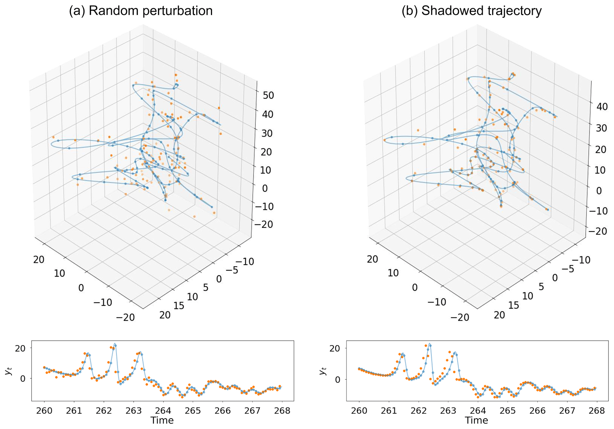
Figure 11 Comparison of the two different types of observations used in the data assimilation experiments. We show the observation space for the benchmark observations case (y_e, y_t, Y). A selection of 800 time steps (100 observations) of the control model (blue line) and values at the observation times (blue dots) are shown in both plots, along with the actual observations used (orange dots). The top figures show behaviour along the attractor and the bottom panels show y_t in time. (a) Observations formed by random perturbations to control run points. (b) Observations taken from a trajectory which shadows the control run.

We repeat the observation experiments of the previous three sections: benchmark observations, atmospheric observations, and ENSO observations. We only focus on the full-rank and variable CLV methods. When using correlated observational errors in any ensemble Kalman filtering method, a larger inflation value and ensemble size are needed to avoid ensemble collapse. We find that for the standard ETKF method increasing the ensemble size to 11 members is sufficient. To facilitate a direct comparison, we therefore also use this ensemble size for the CLV experiments. The inflation value varies slightly with the different observation cases. The setup and results of the experiments are shown in Table 5.

Table 5 Summary metrics of DA experiments using a right-transform matrix (Eq. 15) and shadowed trajectory as observations. We set the observation error covariances to the standard values as in Yoshida and Kalnay (2018). Parameters: assimilation window 0.08, 11 ensemble members, inflation as noted in the table.

When using the benchmark observation set from the shadowed trajectory, the variable CLV method outperforms the full-rank method. This shows improvement over the case with random observation errors discussed in Sect. 5.2, where the variable CLV method performed slightly worse than the full rank. For the atmosphere observation case, we again observe similar performance when using the variable CLV method and the full rank, with the largest reduction of average RMSE in the ocean subsystem. The major change in the ENSO observation case from the random observational error experiments in Sect. 5.4 is that when using the shadowed trajectory observations the variable CLV method no longer fails. There is still difficulty in accurately calculating the first CLV from the extratropical subsystem being unconstrained; however, the correlation in the errors of the tropical and ocean subsystems provides additional information about the underlying nonlinear error growth. We observe that the variable CLV method performs comparably to the full rank, with a slightly larger average RMSE in the ocean subsystem (and subsequently the full). The inability to track the extratropical subsystem can once again be seen through the decrease in average local dimension.

5.6 Extratropical observations

We finally consider the case where one subsystem is fully observed and the others are completely unobserved. We choose to observe the extratropical subsystem, as it is the most extreme case with weakly coupled fast dynamics. Due to the difficulty of constraining the full system with such minimal observations, the assimilation window is reduced to 0.02 and we use perfect observations. In other words, we do not add any perturbations to the control run when making the observation. Having more accurate (mean) observations was shown in Sect. 5.4 to improve the performance of the unobserved subsystems in the assimilation.

It is also clear from the previous experiments that the inability to constrain unobserved subsystems leads to a collapse in dimension and correspondingly a collapse in the covariances. A collapse in covariance is commonly avoided through the use of inflation (Anderson and Anderson, 1999; Hamill et al., 2001; Carrassi et al., 2008; Raanes et al., 2019). While a static background inflation avoids full covariance collapse, we are interested here in the covariance collapse related only to specific subsystems which are not being constrained. For such a case, we argue that the forecast error covariance matrix should be scaled by a factor relating to the ensemble performance at each analysis step. In other words, when an individual subsystem is not being constrained, the covariances should be increased in the calculation of the Kalman gain, analogous to the approach outlined by Miller et al. (1994) for the strongly nonlinear Lorenz '63 system. In their study the authors find that the forecast error covariance is often underestimated in such highly nonlinear systems, particularly when the model is in a region of phase space subject to transitions. Subsequently, the Kalman gain is underestimated. The authors account for this by including the third and fourth moments of anomalies in the Kalman gain calculation.

Here we introduce a new method for adaptive scaling of the Kalman gain. Rather than explicitly calculating higher moments of the anomalies, we account for the underestimation through a spread-dependent factor which balances our forecast error covariance P^f and observation error variance R accordingly, the idea being that a larger spread implies we have underestimated the covariances, and vice versa. We note that this adaptive scaling is different to traditional inflation as it does not directly adjust the underlying ensemble spread. We use this in conjunction with the static background inflation of 1 % to avoid total ensemble collapse.

We scale the Kalman gain in the following way:

$$\begin{array}{}\text{(27)}& \widehat{\mathbf{K}}={\displaystyle \frac{\left|\right|{\mathbf{P}}^{\mathrm{f}}\left|\right|{\mathbf{P}}^{\mathrm{f}}{\mathbf{H}}^{\mathrm{T}}}{\left|\right|{\mathbf{P}}^{\mathrm{f}}\left|\right|{\mathbf{HP}}^{\mathrm{f}}{\mathbf{H}}^{\mathrm{T}}+\mathbf{R}}},\end{array}$$

or equivalently

$$\begin{array}{}\text{(28)}& \widehat{\mathbf{K}}={\mathbf{P}}^{\mathrm{f}}{\mathbf{H}}^{\mathrm{T}}[{\mathbf{HP}}^{\mathrm{f}}{\mathbf{H}}^{\mathrm{T}}+{\displaystyle \frac{\mathbf{R}}{\left|\right|{\mathbf{P}}^{\mathrm{f}}\left|\right|}}{]}^{-\mathrm{1}}.\end{array}$$

Here the scaling factor is the Frobenius norm of P^f=(X^f)(X^f)^T, where X^f is the ensemble spread matrix defined by Eq. (10b). This rescaling factor is mathematically similar to the K-factor adaptive quality control procedure introduced by Sakov and Sandery (2017) and the β-factor rescaling of the background error covariances introduced by Bowler et al. (2013). The K-factor method was used to account for inconsistencies in observations and therefore uses an adaptive observation error covariance R that takes into account innovation size at each analysis step, while the β-factor is a deflation to the forecast error covariance matrix to avoid the underestimation of the ensemble spread ($\mathrm{0}<\mathit{\beta }<\mathrm{1}$). Both the K-factor procedure and the β-factor multiplier can be shown to have the same scaling effect on the Kalman gain K defined by Eq. (9a) as the adaptive scaling presented here, with the difference in that the modified $\widehat{\mathbf{K}}$ in Eq. (28) takes into account both effects: small $\left|\right|\left({\mathbf{X}}^{\mathrm{f}}\right)\left({\mathbf{X}}^{\mathrm{f}}{)}^{\mathrm{T}}\right||$ behaves like the β-factor and large $\left|\right|\left({\mathbf{X}}^{\mathrm{f}}\right)\left({\mathbf{X}}^{\mathrm{f}}{)}^{\mathrm{T}}\right||$ behaves like the K-factor. We discuss the limiting behaviour of this adaptive scaling method in terms of the increment size and analysis error covariance in Appendix A.

Due to the fact that only the Kalman gain is being adjusted, for ease of implementation we use the ESRF method introduced in Sect. 4.1. This allows for the left-transform matrix to be calculated with the modified Kalman gain:

$$\begin{array}{}\text{(29)}& \mathbf{T}=(\mathbf{I}-\widehat{\mathbf{K}}\mathbf{H}{)}^{\mathrm{1}/\mathrm{2}}.\end{array}$$

We apply the adaptive gain to both the full-rank (nine CLVs) and variable-rank formulations of the covariance matrix. The results of the variable-rank experiments with and without adaptive gain are shown in Fig. 12 and the error statistics of all four experiments are listed in Table 6.

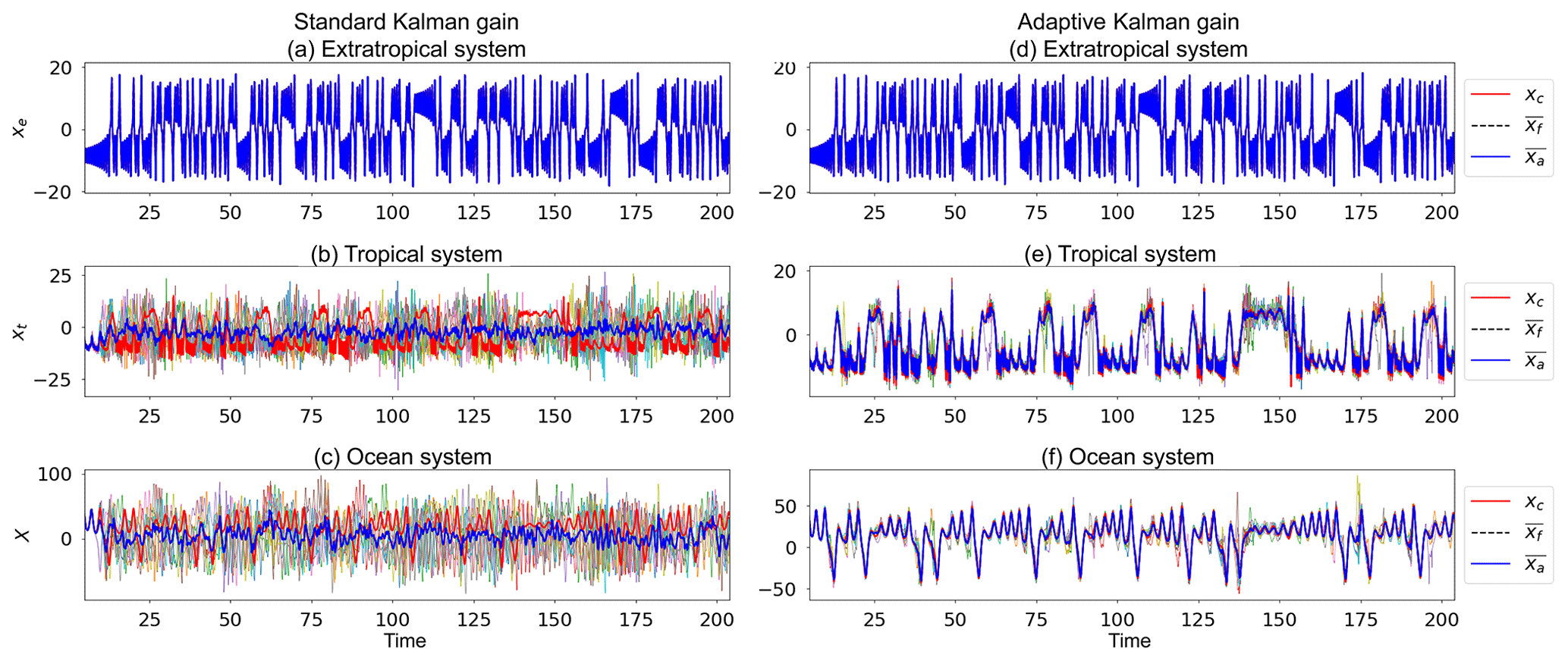
Figure 12 Trajectories of DA experiments using variable CLVs, left-transform matrix (Eq. 17b), and perfect observations from the extratropical subsystem of a control run ($x_{\mathrm{e}},y_{\mathrm{e}},z_{\mathrm{e}}$), with (a–c) the standard Kalman gain (Eq. 9a) and (d–f) the adaptive Kalman gain (Eq. 28). Trajectories shown are control run (red), ensemble mean (blue), and individual ensemble members (multicoloured). For conciseness we only show the results for the x coordinate of each subsystem. The other two coordinates behave similarly. Parameters: assimilation window 0.02, inflation factor 1 %, 10 ensemble members, observation error covariance R=I₄.

Table 6 Summary metrics of DA experiments using a left-transform matrix (Eq. 17b) and the full extratropical subsystem as observations (x_e, y_e, z_e). We use perfect observations (no random error added to the control run) with the observation error covariances set to the standard values as in Yoshida and Kalnay (2018). Parameters: assimilation window 0.02, inflation factor 1 %, 10 ensemble members.

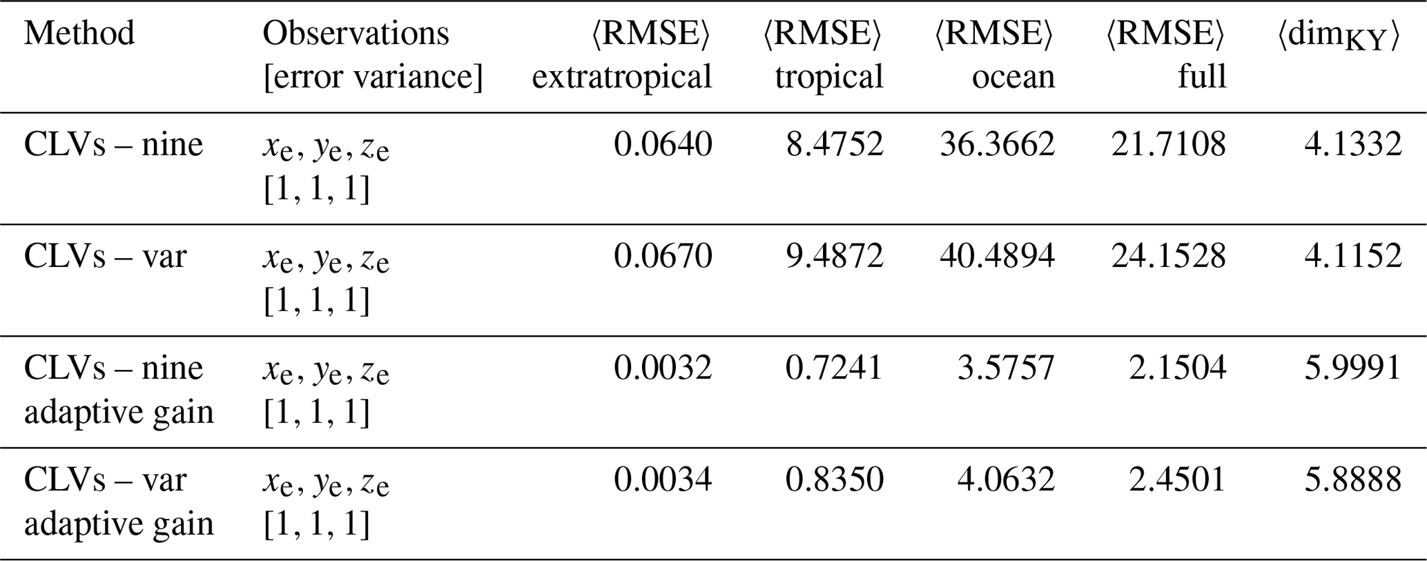
We see from Fig. 12 that there is a remarkable improvement when using the adaptive gain method. Not only is the ensemble spread reduced in the unobserved subsystems, but the ensemble mean is also able to track the control run. This improvement in tracking the control run is exemplified in Table 6 with a significant reduction in the average RMSE of individual subsystems. As expected, the average dimension is also significantly increased.

6 Concluding remarks

This study presents an initial understanding of the transient dynamics associated with the Kalman filter forecast error covariance matrix for nonlinear multiscale coupled systems. We have explored the varying rank of the error covariance matrix related to the transient growth in the stable modes of the system, and in particular the applicability of this varying rank to different configurations of strong CDA. Additionally, we have shown the large impact of using isolated observations and cross-domain covariances in such a coupled system. The cross-covariances are significantly underestimated when the observed subsystems are weakly coupled to the unobserved ones; however, this can be compensated through either reduced observational error or the use of an adaptive scaling of the Kalman gain.

The dynamical properties of strongly coupled DA in a multiscale system were investigated through a low-dimensional nonlinear chaotic model to represent the interactions between the extratropical atmosphere, ocean, and tropical atmosphere–ocean interface. The model contains significant spatio-temporal scale separations between the subsystems, as well as varying coupling strengths. We introduced a local dimension measure, namely the Kaplan–Yorke dimension calculated using FTLEs, to specify the appropriate rank of the forecast error covariance matrix at each analysis step. We have shown that through using time-varying CLVs to form a reduced-rank forecast error covariance matrix, comparable results to the full-rank ETKF and ESRF schemes are achievable.

We considered a benchmark experiment previously explored in Yoshida and Kalnay (2018) to examine the most effective number of CLVs needed to form the forecast error covariance matrix. We found that when using less than full rank, the variable amount based on local dimension performed the best. We also found there was not significant improvement when increasing to full rank. In particular, we found that spanning the space comprised of the asymptotic unstable, neutral, and first weakly stable mode (five CLVs in this case) performed worse than using either dimension measure (asymptotic and local). This suggests that significant growth occurring in more than one weakly stable mode is important when capturing short-term dynamics of highly nonlinear systems. We therefore see improvement when implementing a rank based on local dimension over asymptotic dimension; however, all methods produce successful results in this case, where all subsystems are sampled in the observations.

We then tested the effectiveness of the reduced-rank forecast error covariance matrix in strong CDA when a subsystem is completely unobserved, i.e. using only cross-covariances to determine the increment of the unobserved system. The first set of these experiments used observations from the two atmosphere subsystems, extratropical and tropical, while the ocean was left completely unobserved. In this case we found that the DA succeeded in constraining the system to the observations when using the full rank, asymptotic dimension, and local dimension to determine the rank of the covariance matrix; however, the variable-rank method performed better than the fixed-rank methods. The second set of experiments consisted of ENSO observations or observations from the strongly coupled tropical and ocean subsystems only. In this case, the observational errors and weak coupling to the extratropical subsystem caused the reduced-rank experiment to fail. The full-rank experiment succeeded in tracking the tropical and ocean subsystems but left the extratropical subsystem unconstrained. This resulted in a collapse of the variance in the ensemble mean and a subsequent reduction in the average dimension. However, we found that reducing the observational error variance of the tropical subsystem provided an increase in ensemble mean variance of the extratropical subsystem and therefore an increase in the average dimension. Reducing the observational error variance of the ocean did not provide a significant improvement since it is only indirectly coupled to the extratropical subsystem.

The effect of correlated observational errors was also explored. We constructed a trajectory which shadowed the control run and used this as our observational set, repeating all the previous experiments with different observation subsets. Since the correlated errors preserve the underlying dynamical structure of the system, we found that the reduced-rank method based on local dimension was the most successful in all the experiments when compared to those using random observational error. This included the ENSO observations case, where the extratropical subsystem remained unconstrained.

Finally, we showed that when only observing the extratropical subsystem, the unobserved subsystems could not be constrained due to their weak or indirect coupling to the observations. This manifested as an overall reduction in dimension as well as a collapse in the cross-domain covariances. In order to counter the covariance and dimension collapse, we introduced a novel scheme for adaptive Kalman gain scaling. This adaptive scaling is based on a measure of the overall spread of the system, therefore accounting for unobserved subsystems that have become unconstrained. Through use of the adaptive scaling the weakly coupled unobserved subsystems were able to be relatively constrained, and moreover the ensemble mean of the unobserved subsystems was able to track the control run. The adaptive scaling introduced here should be tested on additional systems with weak coupling in order to assess its general applicability, although care may need to be taken in the choice of the norm.

We now turn to the implications for more realistic high-dimensional systems. It has been shown that when using a finer model resolution (increasing dimension) there is an increase in near-zero asymptotic Lyapunov exponents (De Cruz et al., 2018). We observed through the examination of the dynamical properties of the coupled Lorenz system that the stable yet near-zero exponents have the largest temporal variability, which affects the local dimension. As the number of near-zero exponents increases, we may expect that the temporal variability in dimension will increase further. This would have strong implications for the necessary rank of the forecast error covariance and the subsequent number of ensemble members. It is not implausible that the number of ensemble members could vary significantly in time. In such a case where the model's degree of freedom is much larger than its effective dimension, the projection onto CLVs becomes even more effective. This would ensure the ensemble perturbations lie in subspaces associated with error growth at the given time and that the directions of error growth are sufficiently sampled. Such improvements in modelling error growth of high-dimensional atmospheric systems have already been seen through the use of finite-time normal modes (Wei and Frederiksen, 2005). There is still more work to be done on how CLVs relate to meteorological and climatic events in such models, similar to the blocking studies of Schubert and Lucarini (2016). Future work should also consider the numerical cost of CLV calculation and methods to increase efficiency for high-dimensional systems.

The adaptive gain result presented here highlights the utility of ensemble filtering methods. While the ensemble mean of the subsystems manages to track the control run, the individual members are not so constrained. The variability in the spread of the ensemble members can provide a measure for uncertainty of the corresponding subsystem at a given region in phase space. Additionally, the ability to constrain the ensemble mean of the system from only observations of the weakly coupled fast subsystem is a new result for strong CDA. While dynamically this is intuitive (accurate knowledge of the fast dynamics of a system is sufficient to reconstruct the full attractor), this has not previously been shown to be achievable in DA experiments. If such a scheme could be shown to scale to high-dimensional climate models, then accurate and frequent atmospheric observations could potentially be sufficient to constrain the full system. For this reason it is important that the scheme be analysed for general applicability and tested on a variety of coupled dynamical systems.

Appendix A: Limiting behaviour of adaptive Kalman gain scaling

We address the implication of the adaptive Kalman gain scaling for the two extreme cases: ensemble collapse ($\left|\right|\left({\mathbf{X}}^{\mathrm{f}}\right)\left({\mathbf{X}}^{\mathrm{f}}{)}^{\mathrm{T}}\right||\to \mathrm{0}$) and ensemble divergence ($\left|\right|\left({\mathbf{X}}^{\mathrm{f}}\right)\left({\mathbf{X}}^{\mathrm{f}}{)}^{\mathrm{T}}\right||\to \mathrm{\infty }$).

1. $\left|\right|\left({\mathbf{X}}^{\mathrm{f}}\right)\left({\mathbf{X}}^{\mathrm{f}}{)}^{\mathrm{T}}\right||\to \mathrm{0}$
   We consider the Kalman gain in the form

   $$\begin{array}{}\text{(A1)}& \mathbf{K}=\mathit{\delta }{\mathbf{P}}^{\mathrm{f}}{\mathbf{H}}^{\mathrm{T}}[\mathit{\delta }{\mathbf{HP}}^{\mathrm{f}}{\mathbf{H}}^{\mathrm{T}}+\mathbf{R}{]}^{-\mathrm{1}},\end{array}$$

   where $\mathit{\delta }=\left|\right|\left({\mathbf{X}}^{\mathrm{f}}\right)\left({\mathbf{X}}^{\mathrm{f}}{)}^{\mathrm{T}}\right||$ and the subscript from Eq. (9a) have been dropped for brevity. For δ≪1, Eq. (A1) can be expanded to

   $$\begin{array}{}\text{(A2)}& \begin{array}{rl}\mathbf{K}& =\mathit{\delta }{\mathbf{P}}^{\mathrm{f}}{\mathbf{H}}^{\mathrm{T}}[{\mathbf{R}}^{-\mathrm{1}}-\mathit{\delta }{\mathbf{R}}^{-\mathrm{1}}{\mathbf{HP}}^{\mathrm{f}}{\mathbf{H}}^{\mathrm{T}}{\mathbf{R}}^{-\mathrm{1}}+\mathcal{O}({\mathit{\delta }}^{\mathrm{2}}\left)\right]\\ & =\mathit{\delta }{\mathbf{P}}^{\mathrm{f}}{\mathbf{H}}^{\mathrm{T}}{\mathbf{R}}^{-\mathrm{1}}-{\mathit{\delta }}^{\mathrm{2}}{\mathbf{P}}^{\mathrm{f}}{\mathbf{H}}^{\mathrm{T}}{\mathbf{R}}^{-\mathrm{1}}{\mathbf{HP}}^{\mathrm{f}}{\mathbf{H}}^{\mathrm{T}}{\mathbf{R}}^{-\mathrm{1}}\\ & +\mathcal{O}\left({\mathit{\delta }}^{\mathrm{3}}\right).\end{array}\end{array}$$

   Letting δ→0, Eq. (A2) simplifies to K=0, the zero matrix. In this case the mean analysis increment and error covariance Eqs. (9b–9c) simplify to

   $$\begin{array}{}\text{(A3)}& {\displaystyle }{\stackrel{\mathrm{‾}}{\mathit{x}}}^a={\stackrel{\mathrm{‾}}{\mathit{x}}}^f,\text{(A4)}& {\displaystyle }{\mathbf{P}}^a={\mathbf{P}}^{\mathrm{f}}.\end{array}$$

   In other words, in the case of collapsed spread, the analysis is equal to the forecast.

2. $\left|\right|\left({\mathbf{X}}^{\mathrm{f}}\right)\left({\mathbf{X}}^{\mathrm{f}}{)}^{\mathrm{T}}\right||\to \mathrm{\infty }$
   We consider the Kalman gain in the form

   $$\begin{array}{}\text{(A5)}& \mathbf{K}={\mathbf{P}}^{\mathrm{f}}{\mathbf{H}}^{\mathrm{T}}[{\mathbf{HP}}^{\mathrm{f}}{\mathbf{H}}^{\mathrm{T}}+\mathit{\delta }\mathbf{R}{]}^{-\mathrm{1}},\end{array}$$

   where $\mathit{\delta }=\frac{\mathrm{1}}{\left|\right|\left({\mathbf{X}}^{\mathrm{f}}\right)\left({\mathbf{X}}^{\mathrm{f}}{)}^{\mathrm{T}}\right||}$. For δ≪1, Eq. (A5) can be expanded to

   $$\begin{array}{}\text{(A6)}& \begin{array}{rl}\mathbf{K}& ={\mathbf{P}}^{\mathrm{f}}{\mathbf{H}}^{\mathrm{T}}\left[\right({\mathbf{HP}}^{\mathrm{f}}{\mathbf{H}}^{\mathrm{T}}{)}^{-\mathrm{1}}-\mathit{\delta }({\mathbf{HP}}^{\mathrm{f}}{\mathbf{H}}^{\mathrm{T}}{)}^{-\mathrm{1}}\\ & \mathbf{R}({\mathbf{HP}}^{\mathrm{f}}{\mathbf{H}}^{\mathrm{T}}{)}^{-\mathrm{1}}+\mathcal{O}({\mathit{\delta }}^{\mathrm{2}}\left)\right].\end{array}\end{array}$$

   Letting δ→0, Eq. (A6) simplifies to

   $$\begin{array}{}\text{(A7)}& \mathbf{K}={\mathbf{P}}^{\mathrm{f}}{\mathbf{H}}^{\mathrm{T}}({\mathbf{HP}}^{\mathrm{f}}{\mathbf{H}}^{\mathrm{T}}{)}^{-\mathrm{1}}.\end{array}$$

   In this case the mean analysis increment and error covariance Eqs. (9b–9c) become

   $$\begin{array}{}\text{(A8)}& {\displaystyle }{\stackrel{\mathrm{‾}}{\mathit{x}}}^a={\stackrel{\mathrm{‾}}{\mathit{x}}}^f+{\mathbf{P}}^{\mathrm{f}}{\mathbf{H}}^{\mathrm{T}}\left({\mathbf{HP}}^{\mathrm{f}}{\mathbf{H}}^{\mathrm{T}}{)}^{-\mathrm{1}}\right(\mathit{y}-\mathbf{H}{\stackrel{\mathrm{‾}}{\mathit{x}}}^f),\text{(A9)}& {\displaystyle }{\mathbf{P}}^a=(\mathbf{I}-{\mathbf{P}}^{\mathrm{f}}{\mathbf{H}}^{\mathrm{T}}({\mathbf{HP}}^{\mathrm{f}}{\mathbf{H}}^{\mathrm{T}}{)}^{-\mathrm{1}}\mathbf{H}){\mathbf{P}}^{\mathrm{f}}.\end{array}$$

   Recall that y are the observations defined by y=Hx, where x is the truth (the observation error has implicitly been set to zero in the case of large spread). For a function ℱ with a Taylor series expansion operating on two arbitrary matrices A and B, we have the following identity:

   $$\begin{array}{}\text{(A10)}& \mathcal{F}\left(\mathbf{AB}\right)\mathbf{A}=\mathbf{A}\mathcal{F}\left(\mathbf{BA}\right).\end{array}$$

   Taking A=H, B=P^fH^T, and ℱ the inverse function, we can simplify (A8–A9) to

   $$\begin{array}{}\text{(A11)}& {\displaystyle }{\stackrel{\mathrm{‾}}{\mathit{x}}}^a=\mathit{x},\text{(A12)}& {\displaystyle }{\mathbf{P}}^a=\mathbf{0}.\end{array}$$

   In such a case, all ensemble members are adjusted to the same value as inferred from the observations.