the Creative Commons Attribution 4.0 License.
the Creative Commons Attribution 4.0 License.
 | 27 Apr 2020
Detecting dynamical anomalies in time series from different palaeoclimate proxy archives using windowed recurrence network analysis
Jaqueline Lekscha
Reik V. Donner
Analysing palaeoclimate proxy time series using windowed recurrence network analysis (wRNA) has been shown to provide valuable information on past climate variability. In turn, it has also been found that the robustness of the obtained results differs among proxies from different palaeoclimate archives. To systematically test the suitability of wRNA for studying different types of palaeoclimate proxy time series, we use the framework of forward proxy modelling. For this, we create artificial input time series with different properties and compare the areawise significant anomalies detected using wRNA of the input and the model output time series. Also, taking into account results for general filtering of different time series, we find that the variability of the network transitivity is altered for stochastic input time series while being rather robust for deterministic input. In terms of significant anomalies of the network transitivity, we observe that these anomalies may be missed by proxies from tree and lake archives after the non-linear filtering by the corresponding proxy system models. For proxies from speleothems, we additionally observe falsely identified significant anomalies that are not present in the input time series. Finally, for proxies from ice cores, the wRNA results show the best correspondence to those for the input data. Our results contribute to improve the interpretation of windowed recurrence network analysis results obtained from real-world palaeoclimate time series.
- Article
(6099 KB) - Full-text XML
-
Supplement
(582 KB) - BibTeX
- EndNote


Palaeoclimate proxy time series from archives such as trees, lakes, speleothems, or ice cores play an important role in past climate reconstructions (Bradley, 2015). Apart from information on climatic boundary conditions such as local and global mean temperatures and precipitation sums, the analysis of the proxy time series using non-linear methods offers the possibility of studying dynamical anomalies in past climate variability (Marwan et al., 2002, 2003; Trauth et al., 2003; Marwan et al., 2009; Donner et al., 2010b; Franke and Donner, 2017). Due to the limitations of palaeoclimate proxy time series in terms of non-uniform sampling of the data points, uncertainties in dating and measurement, the contamination with noise, and the often non-unique interpretation of the climate signal within the proxy, not all methods are suitable for gaining reliable information from all data (Goswami et al., 2018; Lekscha and Donner, 2018).
Windowed recurrence network analysis (wRNA) has already been successfully used to detect dynamical anomalies in time series from different palaeoclimate archives (Donges et al., 2011a, b; Eroglu et al., 2016; Lekscha and Donner, 2018). But it has also been observed that this method often yields high numbers of false positive significant points and that not all palaeoclimate archives give equally robust results. In order to improve the interpretation of results obtained with wRNA for real-world time series, we here systematically test the suitability of the approach for analysing palaeoclimate data from different types of archives by employing proxy system models.
Proxy system models are forward models that simulate the formation of a palaeoclimate proxy based on the systemic understanding of that proxy (Evans et al., 2013). That is, given the climate input variables, the proxy system model outputs a proxy time series. We here use intermediate complexity models for tree ring width, branched glycerol dialkyl glycerol tetraethers in lake sediments, and the isotopic composition of speleothems and ice cores (Tolwinski-Ward et al., 2011; Dee et al., 2015, 2018). We first create artificial climate input time series with different properties. In particular, we consider two stochastic processes, Gaussian white noise and an autoregressive process of order 1, and two non-stationary time series from the paradigmatic Rössler and Lorenz systems. Additionally, we use climate input from the Last Millennium Reanalysis project as an estimate of realistic past climate variability (Hakim et al., 2016; Tardif et al., 2019). We then compare the input and the model output with respect to the properties of the time series and the results of wRNA. To quantify significant dynamical anomalies, we use an areawise significance test that was recently introduced for wRNA (Lekscha and Donner, 2019).
With this work, we want to contribute to a better understanding and an improved interpretation of results obtained with wRNA for palaeoclimate applications. We first introduce our analysis framework in Sect. 2, the proxy system models in Sect. 3, and the input time series in Sect. 4. Then, we show and discuss the results of the wRNA for the different input and model output time series in Sect. 5 before we present our main conclusions in Sect. 6. Additional information and figures are included in the Supplement accompanying this paper.
2.1 Phase space reconstruction
The first step when analysing data using recurrence-based approaches is to reconstruct the higher-dimensional phase space of the system from the measured univariate time series x(t) with observations made at times . For this, we use uniform time delay embedding (Takens, 1980; Packard et al., 1980) which relates the higher-dimensional coordinates of the system's phase space to delayed versions of the measured, univariate time series
Here, m denotes the embedding dimension and τ is the embedding delay. The embedding theorem of Takens guarantees that, when choosing the embedding dimension larger than twice the box-counting dimension of the original attractor, the reconstructed and original systems' attractors are related by a smooth one-to-one coordinate transformation with smooth inverse, independent of the choice of the delay (Takens, 1980). That is, analysing the dynamics in the reconstructed phase space can give information on the original system dynamics. Still, this theorem only provides a sufficient condition for the embedding dimension, while lower-dimensional embeddings may also give useful information about the system's dynamics.
In practical applications, however, the box-counting dimension of the original attractor is usually unknown and the data are finite and subject to noise such that the choice of the embedding parameters plays an important role in the quality of the phase space reconstruction. In particular, the embedding dimension can be estimated using the method of false nearest neighbours (Kennel et al., 1992), while the first zero of the autocorrelation function or the first minimum of the mutual information can serve as an estimate for a suitable embedding delay (Abarbanel et al., 1993; Fraser and Swinney, 1986; Kantz and Schreiber, 2004). We here use an embedding dimension of m=3 as a compromise between the number of available data points and the minimum number of independent coordinates as indicated by the false nearest neighbour criterion. To estimate the embedding delay, we use the first zero of the global lagged autocorrelation function.
2.2 Windowed recurrence network analysis
We analyse the embedded time series x(t) by means of windowed recurrence network analysis (wRNA), using a sliding window approach and dividing the embedded time series into windows of width W with mutual offset dW. For each of those windows, we construct a network from the time series by identifying the different xi=x(ti) as nodes of the network and drawing a link between two nodes xi and xj if they are mutually closer in phase space than some threshold ϵ. For this purpose, we measure the distances in phase space using the maximum norm,
which has, due to its particularly simple form when calculated in Euclidean space, been widely used in recurrence-based analyses. Then, the resulting recurrence network can be described by its adjacency matrix A with entries
where θ(⋅) is the Heaviside function and the delta function δi,j excludes self-loops in the network. Here, we select the threshold adaptively by choosing a fixed edge density ρ=0.05. This means, for every window, we choose the threshold ϵ such that a fraction ρ of all possible links in the network are realised (corresponding to the 100ρ % mutually closest pairs of state vectors).
From the adjacency matrix, we can estimate various network properties. In the course of this work, we will restrict ourselves to the network transitivity
which gives the probability that two randomly chosen neighbours of a randomly chosen node are mutually connected. Network transitivity is particularly well suited for detecting dynamical anomalies in non-stationary time series, since this network measure has been shown to be closely related to the dimensionality of the system dynamics, in particular, when using the maximum norm to measure distances in phase space (Donner et al., 2010a, 2011b). Specifically, the quantity then corresponds to a generalised fractal dimension (Donner et al., 2011a). Thus, low values of the network transitivity can be related to higher-dimensional dynamics and vice versa.
For the analysis performed here, we repeat the wRNA for different values of the window width with step size ΔW=1 in order to check the robustness of the results for this analysis parameter. Thus, the resulting values of the network transitivity can be stored in some matrix Q which is of size , with NW being the number of window widths for which the analysis has been performed and N′ being the number of windows into which the original time series is divided. We choose the offset of the windowed analysis to be always dW=1.
2.3 Significance testing and confidence levels
In order to identify dynamical anomalies from the resulting network transitivity, we first perform a pointwise significance test using random shuffling surrogates. That is, for every window width W, we randomly draw Ns=1000 times W embedded state vectors from x(t) and calculate the network transitivity of this set of W state vectors. We then take the empirical 2.5th and 97.5th percentiles from the Ns realisations to obtain a two-sided confidence interval of spw=95 %. All transitivity values of the original analysis results that fall outside this interval are considered to show pointwise significant anomalies; that is, the null hypothesis of the corresponding values of transitivity resulting from random data with the same amplitude distribution as the original data is rejected. The result of this pointwise significance test can be summarised in the binary significance matrix Spw of the same size as the matrix of the transitivity results Q. The entries of Spw equal one if the corresponding value of the transitivity has been found to be pointwise significant, and zero otherwise.
As intrinsic correlations of the analysis results in both the time domain (due to the short offset dW) and the window width domain can lead to patches of false positives in the pointwise significance matrix, we additionally perform an areawise significance test (Lekscha and Donner, 2019; Maraun et al., 2007). A pointwise significant point is defined as areawise significant if all neighbouring points within a given rectangle are also pointwise significant, i.e. if the pointwise significant point lies within a patch of pointwise significant points that is larger than this rectangle. The side lengths of the rectangle depend on the intrinsic correlations of a chosen null model that are estimated as described in detail in Lekscha and Donner (2019).
Here, we employ a data-adaptive null model using iterative amplitude-adjusted Fourier transform surrogates of the original time series (Schreiber and Schmitz, 2000). That is, we test whether the same analysis results could have been obtained from data with the same amplitude distribution and linear correlation structure as the original data but that are otherwise random, i.e. originate from linear stochastic processes with prescribed correlations.
Forward modelling of palaeoclimate proxies offers the possibility of gaining insights into the underlying processes that influence the sensitivity of a given proxy to climate variations and can thus be used to investigate characteristic properties of time series of different palaeoclimate archives and their implications for further analyses. We here use four models for typical proxies from tree rings, lake sediments, ice cores and speleothems, respectively, in order to test how well dynamical anomalies can be identified when applying wRNA to time series originating from those archives.
Generally, a proxy system model can be divided into an environment, a sensor, an archive and an observation sub-model (Evans et al., 2013). The environment model can be used to model the environmental factors that the archive is sensitive to using the climatic input variables. The sensor model then describes how the archive reacts to the environment, and the archive model accounts for how this reaction is written into the archive. Finally, an observation model can be used to simulate uncertainties in dating or measurements. Here, depending on the archive, we use different combinations of the environment and sensor and archive sub-models, while neglecting possible dating and measurement uncertainties. In the following, we will give a brief overview of the model structures and parameters. A full description of the models can be found in the corresponding references.
3.1 Tree rings
Tree rings are one of the most important archives for palaeoclimate reconstructions of the last millennium (Bradley, 2015; St. George, 2014; St. George and Esper, 2019). To model the tree ring width as a function of time at a particular site, we use the intermediate-complexity Vaganov-Shashkin-Lite (VS-Lite) model (Tolwinski-Ward et al., 2011). This is a reduced version of the full Vaganov–Shashkin model (Vaganov et al., 2006) and requires monthly input data of temperature T and either precipitation P or soil moisture M. Additional model parameters are thresholds for temperature and soil moisture below which growth is not possible and above which growth is optimal (), the latitude of the site Φ, and integration start and end months I0 and If that set the period over which climate is responsible for growth in a given year.
If precipitation is given, the leaky bucket model (Huang et al., 1996) is used as an environment model to calculate the soil moisture M(t) based on the water balance in soil. This model requires additional parameters such as the initial moisture content of the soil M0, minimum and maximum soil moisture content Mmin,max, runoff parameters m, α and μ and the root depth dr. The sensor model for the tree ring width then basically relies on the principle of limiting factors (Fritts, 1976); that is, it assumes that tree ring growth is limited by the resource that is the scarcest for optimal growing conditions, i.e. in this case, the temperature or the soil moisture. A temperature-based growth response is calculated as
and similarly, a growth response gM(t) is calculated for soil moisture. In addition, a third insolation-based growth response gE(t) is calculated based on the mean of the normalised lengths of the day for each month. The total growth response g(t) of the tree to the climatic input is then given as the minimum of the temperature- and moisture-based growth responses modulated by the insolation-based growth response,
To obtain the annual growth response from those monthly data, the model integrates the growth response g(t) over those months that are specified as the start and end months I0 and If. Finally, the annually resolved time series of tree ring width anomalies is obtained by normalising the annual growth response to zero mean and unit variance.
It should be noted that this model does not take into account juvenile tree growth. Real tree ring width data are of course subject to juvenile growth and the effect is usually subtracted from the measured data. Problems arising from this are thus disregarded in the model, which we will further address when discussing the results for the model.
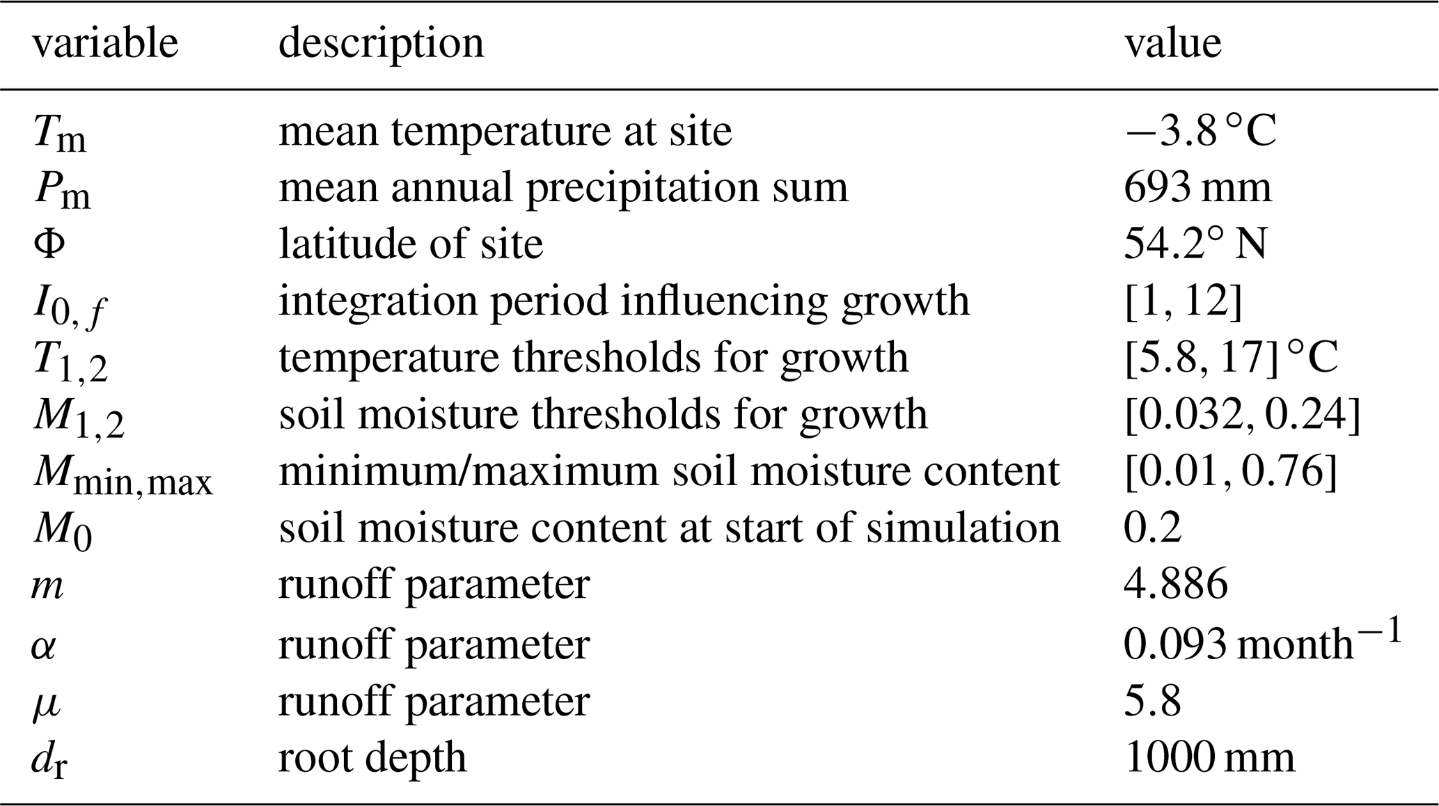
To set the model parameters to realistic values, we use an exemplary real-world data set of a local tree ring width index chronology from eastern Canada (54.2∘ N, 70.3∘ W) that was previously used for regional summer temperature reconstruction (Gennaretti et al., 2014). The quality of this data set with respect to data homogeneity, sample replication, growth coherence, chronology development, and climate signal has been ranked high (Esper et al., 2016). Regional average annual temperature is about C, with average maximum temperatures of 16 ∘C in July and minimum temperatures of C in January. The average annual precipitation sum is 693 mm, with a monthly minimum of about 30 mm in February/March and a maximum of about 100 mm in September. This information has been used in order to choose the mean and standard deviations of the climatic input variables and their annual cycles. An overview of the climate input and also the model parameters is given in Table 1. To determine the threshold parameters, we used the Bayesian parameter estimation as suggested in Tolwinski-Ward et al. (2013). The parameters for the leaky bucket model are chosen as recommended in Tolwinski-Ward et al. (2011).
Table 1Climatic input variables and model parameters for the tree ring width model as derived from the eastern Canada data (Gennaretti et al., 2014).
3.2 Lake sediments
Records from lake sediments are available from many regions worldwide and can provide information about past temperatures and precipitation, depending on the regional boundary conditions and measured proxy (Cohen, 2003). We here model branched glycerol dialkyl glycerol tetraethers (brGDGTs) from lacustrine archives that have been related to air temperatures by using one of the sensor models provided in the PRYSM v2.0 framework (Dee et al., 2018). For this, as model input, a time series of mean annual air temperature T is required.
BrGDGTs are produced by bacteria, and their degree of cyclisation and methylation has been related to soil temperatures, lake pH, and also to mean annual air temperatures (Weijers et al., 2007; De Jonge et al., 2014; Russell et al., 2018). The degree of methylation is quantified by a methylation of the branched tetraether (MBT) index. The sensor model employs the MBT index that only uses 5-methyl isomers. In particular, the calibration of Russell et al. (2018) is used, in which the mean annual air temperature is related to the MBT index via the equation
The archive model then accounts for bioturbation and mixing of the sediments using the TURBO2 model (Trauth, 2013). TURBO2 models the benthic mixing effects on individual sediment particles by assuming that in a mixed layer of a specified thickness on top of a sediment core, instantaneous mixing of the sediment particles occurs, while the rest of the core is not affected by the mixing. In addition to the time series of the sensor model output, the archive model requires three further input parameters, the abundance of the signal carrier over time (abu), the mixed-layer thickness over time (mxl), and the number of fossil foraminifera on which the proxy signal is measured (numb). The model then returns time series of original and bioturbated abundances and corresponding proxy signatures for the original and a second virtual species that is required to keep the total abundance of all species constant over time. The bioturbated proxy signatures of the first species are then used as a final proxy for the mean annual air temperature.
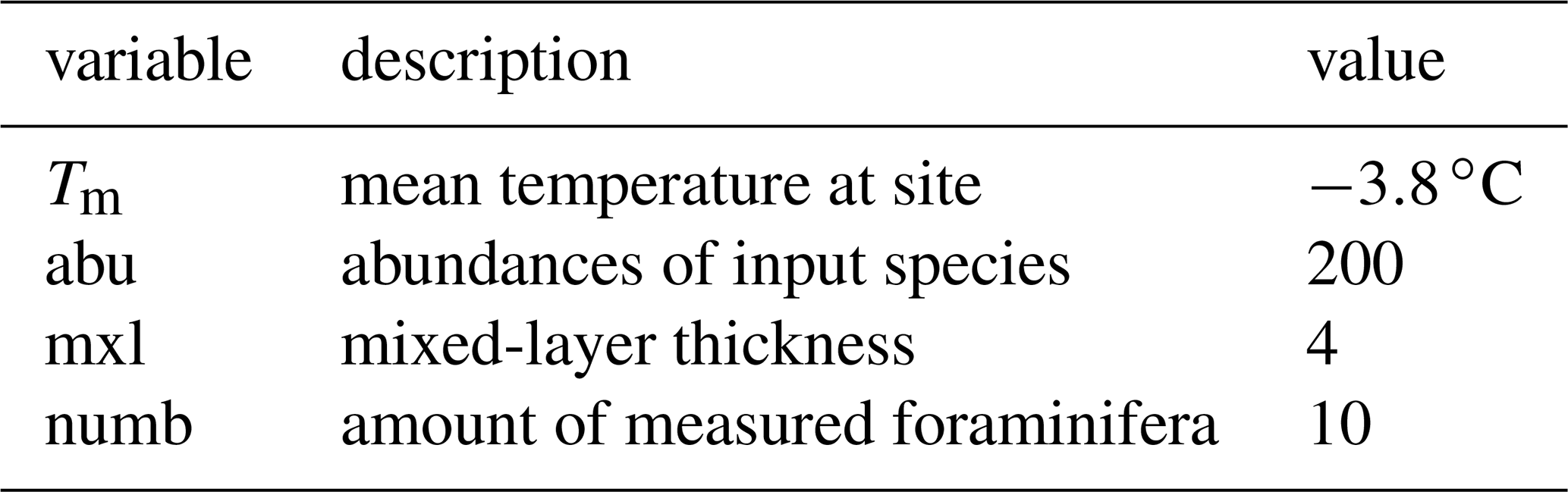
To tune the climatic input variables, we use the climatic setup corresponding to the one used for the tree ring archive in eastern Canada, while for the model parameters, we use typical values for lake sediments that are taken as a default in the PRYSM implementation of the lake archive model (Dee et al., 2018). In particular, it should be noted that for the abundances of the input species and the mixed-layer thickness, we use constant values over time. The climatic and model input parameters are specified in Table 2.
Table 2Climatic input variables and model parameters for the lake sediment model as derived from the eastern Canada data (Gennaretti et al., 2014).
3.3 Speleothems
Oxygen isotope fractions of speleothems have been shown to provide valuable insights into past climate variability (Wong and Breecker, 2015). We here model the isotopic composition of speleothems by using the speleothem model presented within the PRYSM framework (Dee et al., 2015). This intermediate-complexity model is based on the model in Partin et al. (2013) and requires the mean annual temperature T and the mean of the precipitation-weighted annual isotopic composition of the precipitation δ18OP as input. Additionally, the groundwater residence time τgw has to be specified.
The sensor model covers processes in the karst and the cave, while processes in the soil such as evapotranspiration are neglected. The model filters the δ18OP signal by applying an aquifer recharge model to simulate the storage and thus the mixing of water of different ages in the karst. This process is parameterised by the mean transit time τgw. The isotopic composition of the cave water is then given as the convolution (*) of δ18OP with the impulse response of the aquifer recharge model for t>0:
Finally, to obtain the isotopic composition of the flowstone calcite δ18Oc, the model implements a temperature-dependent fractionation (Wackerbarth et al., 2010):
with the temperature Ta being the decadal average of T that is calculated using a Butterworth filter (Zumbahlen, 2008).
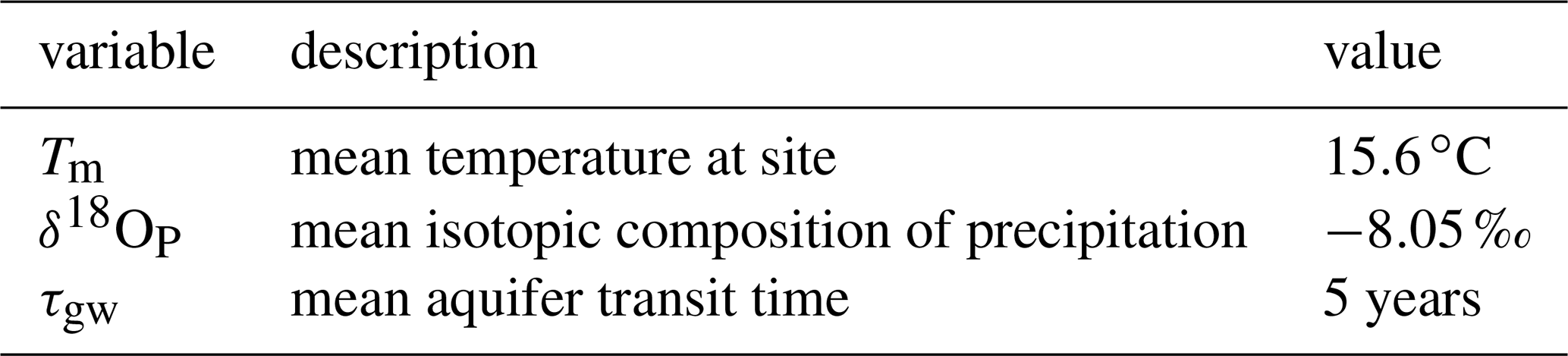
The parameters for the speleothem δ18O model are tuned by using the data of stalagmite DA from Dongge cave (Wang et al., 2005), which is one of the most studied speleothem data sets. Dongge cave is located in southern China (25.3∘ N, 108.1∘ E) at an elevation of 680 m, and the data could be related to the history of the Asian monsoon of the last 9000 years. The proxy values have an average of −8.05 ‰ and the average temperature in the cave is 15.6 ∘C. The mean of the precipitation-weighted isotopic composition of the input is chosen such that the average of the model output data equals the average of the Dongge cave proxy data. There is no information available about the mean transit time, i.e. the time the water has spent inside the karst before entering the cave. We here choose to use an average transit time of 5 years, which is slightly larger than the average sampling rate of the data (4.2 years). An overview of the input variables and model parameters is given in Table 3.
Table 3Climatic input variables and model parameters for the speleothem δ18O model as derived from the Dongge cave data (Wang et al., 2005).
3.4 Ice cores
Proxy time series from ice cores have been used in a variety of contexts to study past climate variability on different timescales (Jouzel, 2013; Thompson et al., 2005). As for the speleothem δ18O, we use the model for ice core δ18O that is implemented and presented within the PRYSM framework (Dee et al., 2015). The model requires the precipitation-weighted mean annual isotopic composition of the precipitation δ18OP as input. Additional parameters are the mean temperature at the site Tm, the altitude of the glacier z, the mean surface pressure p, the mean accumulation rate at the site A, and the total depth of the core hmax which is given by the time span of the observations times the average accumulation rate.
The sensor model corrects the isotopic composition of the precipitation for the altitude of the glacier by using the relation
with a describing the altitude effect. The archive model then accounts for compaction and diffusion within the ice core. First, the density of the core has to be calculated as a function of the depth of the core. For this, an adapted version of the firn densification model by Herron and Langway is used (Herron and Langway, 1980). From the density and the mean temperature Tm, we can then compute the diffusion length σ within the core as a function of the depth h (Johnsen et al., 2000). This, in turn, is used to calculate the final proxy time series δ18Od by convolving the isotopic signal of the ice δ18Oice with a Gaussian kernel function with standard deviation equalling the diffusion length at a given depth,
where the convolution is again denoted by the asterisk (*).
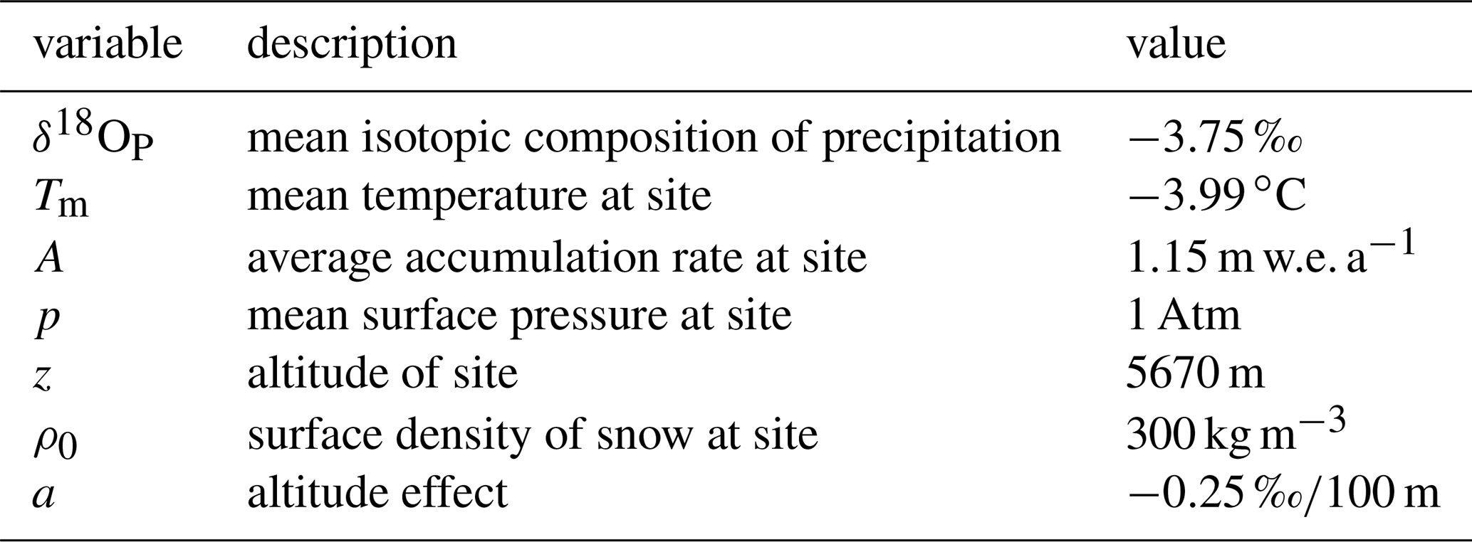
To tune the climatic input variables and model parameters of the ice core δ18O model, we use an exemplary real-world data set of the Quelccaya ice cap (Thompson et al., 2013), which is one of the most studied ice core data sets outside the polar regions. The Quelccaya ice cap is located in the Peruvian Andes ( S, W) at an altitude of 5670 m above sea level. The average accumulation rate is 1.15 m water equivalent per year and the mean δ18Oice is −17.9 ‰. The average annual temperature over the last decade at the Quelccaya ice cap is given as C (Yarleque et al., 2018). An overview of the climatic input variables and the model parameters can be found in Table 4.
Table 4Climatic input variables and model parameters for the ice core δ18O model as derived from the Quelccaya ice cap data (Thompson et al., 2013; Yarleque et al., 2018).
We now introduce the data sets that we use as input for the proxy system models. We first consider two stationary stochastic processes, namely Gaussian white noise (GWN) and an autoregressive process of order 1 (AR(1) process), to evaluate whether such input can lead to the detection of dynamical anomalies in the proxy time series. Then, we consider non-stationary versions of the two well-known Rössler (ROS) and Lorenz (LOR) systems. For all those processes, time series of length N=1000 are independently created to describe temperature, precipitation and precipitation-weighted oxygen isotope fractions as detailed below, where the precipitation is proportional to negative temperature. Additionally, we use data from the last millennium reanalysis project (Hakim et al., 2016; Tardif et al., 2019). Then, as for the tree ring width model monthly input is required, and an annual cycle is added to the temperature and precipitation data. The amplitude of the annual cycle is chosen according to the climatic boundary conditions of the tree ring width index time series from eastern Canada presented in Sect. 3. Finally, yearly means for temperature and sums for precipitation are calculated for those models that require yearly input. The input time series are normalised to zero mean and unit standard deviation, and for each model, the mean is adjusted to the corresponding climatic boundary conditions.
4.1 Gaussian white noise
For the case of GWN, we draw N data points independently at random from the probability distribution
where σ=1 is the standard deviation and μ=0 is the mean of the distribution. We do not expect to detect significant dynamical anomalies from time series created in this way as the process is stationary.
4.2 Autoregressive process of order 1
For the AR(1) process, we create a time series of length N by using the relation
with ϵt a Gaussian random variable with zero mean and constant standard deviation σϵ=0.5. The scaling factor is given as α=0.7 corresponding to the approximate value that we obtained when fitting an AR(1) process to the tree ring width data from eastern Canada (Gennaretti et al., 2014). As an initial condition, we use x(0)=0.3. The resulting time series is normalised to zero mean and unit standard deviation. As for GWN, we do not expect to detect significant dynamical anomalies in the corresponding time series.
4.3 Non-stationary Rössler system
In a next step, we use data from a non-stationary version of the Rössler system which exhibits non-trivial and rich cascades of bifurcations despite its rather simple attractor topology. The Rössler system is defined by the set of ordinary differential equations (ODEs) (Rössler, 1976)
It should be noted that this model is not meant to simulate real-world climate dynamics.
We here use the two fixed parameters a=0.2 and c=5.7 and a time-varying parameter with b0=0.02 and Δb=0.001. We numerically solve this system of ODEs with a temporal resolution of Δt=0.1 for times in the range [0,730], discard the first 300 points and then use every seventh point of the remaining time series of the x component to end up with a time series of length N=1000. As initial conditions we use x(0)=0.5, y(0)=0 and z(0)=0. Again, we normalise the time series to have zero mean and unit standard deviation. The resulting time series and the corresponding Feigenbaum diagram of the stationary system (i.e. ) are shown in the Supplement in Fig. S1.
From the Feigenbaum diagram, it becomes clear that we expect to detect alternating periods of lower- and higher-dimensional dynamics in the time series. In particular, we stress that we do not expect to detect the bifurcation points but periods of outstandingly high- or low-dimensional dynamics in between them as we use random shuffling surrogates for the pointwise significance test.
4.4 Non-stationary Lorenz system
The Lorenz system shows a more complicated attractor topology than the Rössler system and was originally introduced as a simple toy model for atmospheric convection processes (Lorenz, 1963). It is given by the following set of ODEs (Lorenz, 1963):
We here use the setting studied in Donges et al. (2011a) and correspondingly fix the parameters a=10.0 and , while the parameter b is again varied over time as with b0=160.0 and Δb=0.02. We numerically solve this system of ODEs with a temporal resolution of Δt=0.05 for times in the range [0,500] and use every fifth point of the x component of the system to end up with a univariate time series of length N=1000. As initial conditions we use x(0)=10.0, y(0)=10.0 and z(0)=10.0. Again, we normalise the time series to have zero mean and unit standard deviation.
The stationary Lorenz system has been found to exhibit a shift from periodic to chaotic dynamics at b=166.0 (Barrio and Serrano, 2007), while for the transient system as described above, transitions could be detected at b=161.0 and b=166.5 (Donges et al., 2011a). Thus, we expect to detect regimes of more periodic dynamics for b<166.5 and of more chaotic dynamics for b≥166.5 in terms of significantly high and low values of the network transitivity, respectively.
4.5 Last millennium reanalysis data
Finally, we consider reconstructed temperature and precipitation data of the years 501–2000 CE from the Last Millennium Reanalysis project version 2 (Hakim et al., 2016; Tardif et al., 2019), which combines information from general circulation models and from proxy measurements using palaeoclimate data assimilation. As no information about the isotopic composition of the precipitation is available, we only consider the models for tree ring width and lake sediments with this input. From the available global gridded data, we use the standardised, that is, unit-less, ensemble average time series of temperature and precipitation from the grid points with the coordinates closest to those for which we have calibrated the tree and the lake model, that is, at 54∘ N, 70∘ W.
Before studying the different proxy system models, we note that applying some general filtering techniques such as moving average filtering or exponential smoothing to the described stochastic input time series on the one hand and the deterministic input time series on the other hand changes the results of the windowed recurrence network analysis in different ways (not shown here for brevity). For the stochastic time series, the filtering mostly changes the variability of the calculated network transitivity. In particular, filtering an AR(1) process with moving averages produces extended and additional areawise significant patches of high values of the network transitivity. In turn, for deterministic input time series, the variability of the network transitivity remains rather robust under filtering. Furthermore, the results for the network transitivity remain similar when adding white noise to the different input time series up to signal-to-noise ratios of 10 and show increasingly different variability for lower signal-to-noise ratios.
We then turn to the output time series of the different proxy system models which combine linear and non-linear transformations and filtering of the input time series. The different input and model output time series and some remarks on their properties can be found in the Supplement. Figures 1 to 5 show the resulting network transitivity over time for the different time series. Areawise significant points indicating anomalously low or high values of the network transitivity are highlighted by contours.
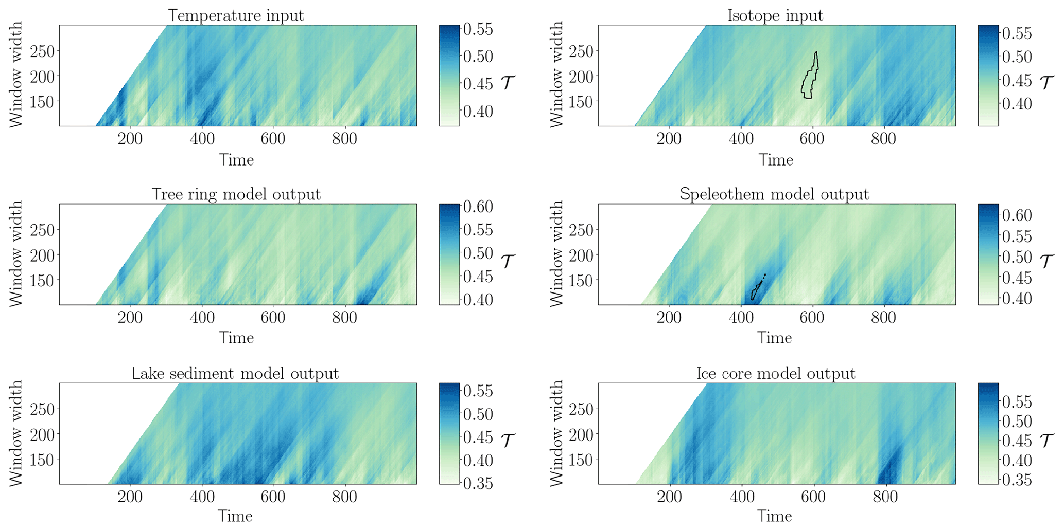
Figure 1Network transitivity (colour-coded) for GWN model input and output with an areawise significance test (contours).
For Gaussian white noise (Fig. 1), we observe the expected changes in the variability of the network transitivity for stochastic input when processing the time series through different filters. For the isotopic composition of the precipitation, we find a patch of areawise significant anomalously low values of the network transitivity, which is a random artifact in this particular realisation of GWN. The outputs of the speleothem and the ice core model do not show this anomaly; i.e. the processing through the model causes the initially significant (false positive) points to be missed and creates an additional patch of areawise significant network transitivity in the case of the speleothem model.
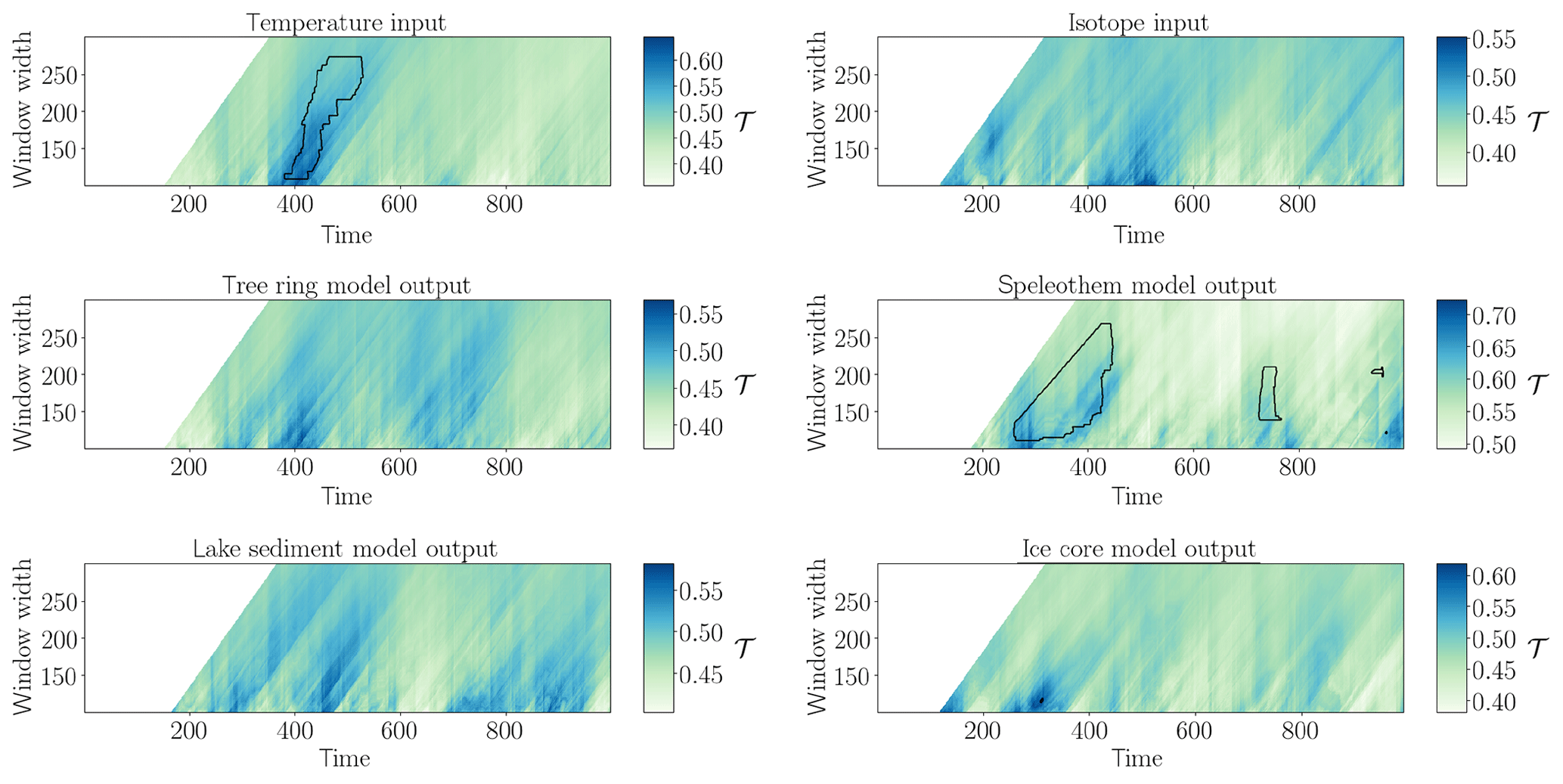
In the case of the AR(1) process (Fig. 2), we observe an areawise significant patch of anomalously high values of network transitivity for the input temperature that is not apparent in the tree ring width and lake sediment model output. For the isotope input, we do not find any areawise significant points, while the speleothem model shows two large and two small falsely identified significant patches of network transitivity. That is, when recalling the results for the filtering of the AR(1) process, we find that the speleothem model seems to particularly involve a way of filtering that produces patches of areawise significant high values of the network transitivity, while the other models rather change the variability of the stochastic input.
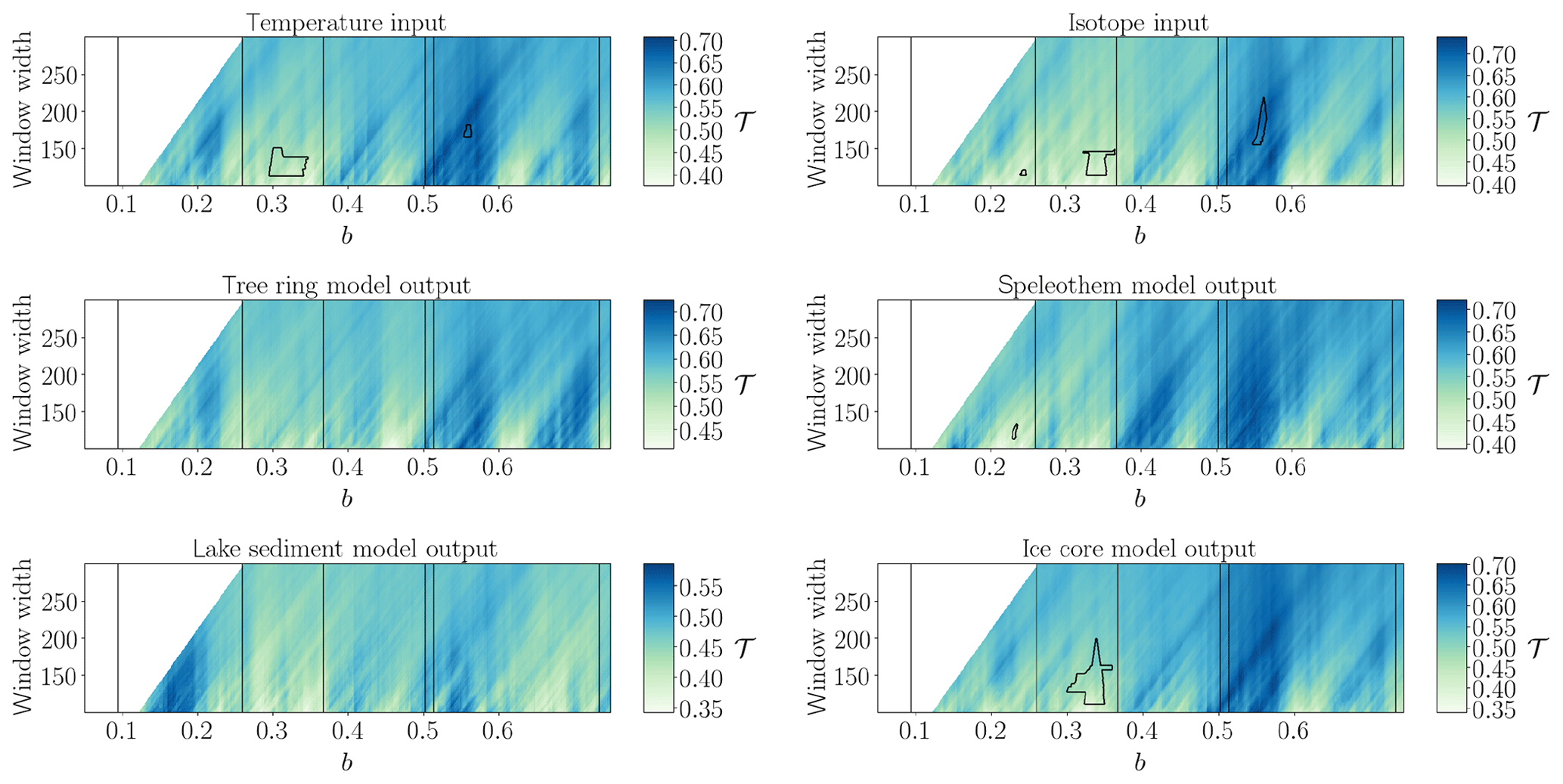
Figure 3Same as in Fig. 1 but for non-stationary Rössler system input. The vertical lines mark the expected bifurcation points identified in the Feigenbaum diagram in Fig. S1.
For the non-stationary Rössler system (Fig. 3), the input time series show areawise significant patches of low network transitivity values in the parameter range and of high network transitivity for . The isotope input has an additional small areawise significant patch around b=0.15. As expected for deterministic input, we observe a much better agreement of the variability of the network transitivity for the input and model output time series than for the two stochastic input and corresponding model output time series. Still, for the tree ring and lake sediment model, the processing through the model prevents the significant points from being detected. The speleothem model output only shows the small areawise significant patch at b=0.15 but not the others, while the output from the ice core model displays the areawise significant patch for .
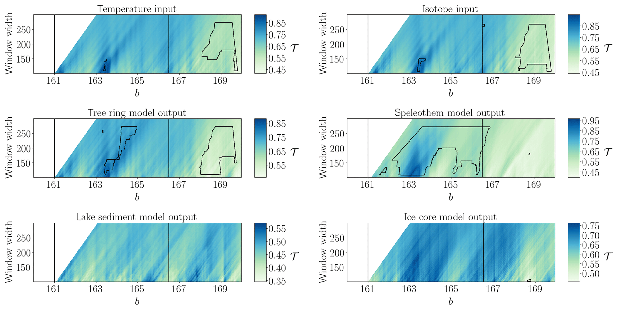
Figure 4Same as in Fig. 1 but for non-stationary Lorenz system input. The vertical lines denote the transitions at b=161.0 and b=166.5 as detected in Donges et al. (2011a).
The input time series of the non-stationary Lorenz system (Fig. 4) exhibits a large patch of areawise significant low values of the network transitivity for high values of b and a small patch of areawise significant high values of the network transitivity around b=163.2. The isotope input shows another small significant patch around b=166.6. The resulting network transitivity for all proxy system model output time series except the one from the lake model reproduces the shift in network transitivity from higher to lower values after b=166.5, as expected for this deterministic input. The tree ring width model output reproduces the large and small patches of significant values of the network transitivity and additionally exhibits another areawise significant patch of high transitivity values close to the small patch. In the speleothem model output, not the low values of the network transitivity at the end of the time series, but rather the high values for , are classified as areawise significant, which might again be related to the particular filtering in the speleothem model favouring areawise significant high values of the network transitivity. The ice core model output only shows a small patch for high values of b and low values of the window width and misses most of the areawise significant points apparent in the isotope input.
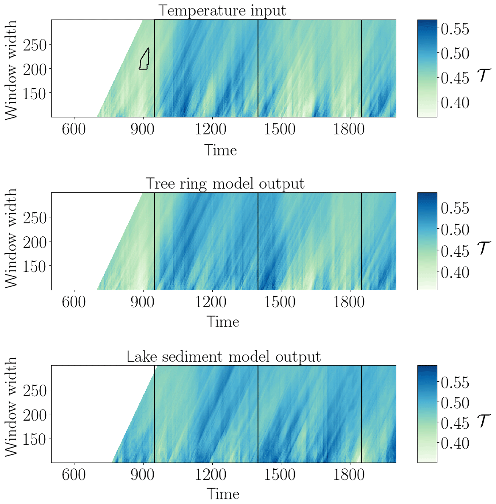
Figure 5Network transitivity (colour-coded) for Last Millennium Reanalysis input at 54∘ N, 70∘ W and corresponding output with an areawise significance test (contours). The vertical lines denote the approximate onset dates of the Medieval Climate Anomaly, the Little Ice Age, and the industrial age, respectively.
For the Last Millennium Reanalysis data temperature input (Fig. 5), we find a patch of areawise significant values of anomalously low values of the network transitivity around the year 900 CE, roughly coinciding with the onset of the European Medieval Climate Anomaly (MCA, denoted by a vertical line at 950 CE). The other vertical lines depict the approximate onset of the European Little Ice Age (LIA) at 1400 CE and the onset of the industrial age at 1850 CE. It should be noted that the timings and imprints of these episodes are known to exhibit substantial regional differences (Franke and Donner, 2017); thus, the reference lines are only for orientation. The model output time series do not show any areawise significant points even though the network transitivity of the model output (and particularly the tree ring width model output) varies similarly to the network transitivity of the temperature input, with higher values during the MCA and lower values during the LIA. The MCA has often be attributed to more stable climate conditions, while the LIA has often been associated with more variable climate conditions even though this imprint has varied locally and has been mainly discussed for Europe. Thus, given the theoretical relation between network transitivity and the dimensionality of the system's dynamics (Donner et al., 2011a), we tentatively conclude that the higher values of the network transitivity during the MCA and the lower values of the network transitivity during the LIA reflect a lower-/higher-dimensional dynamics of the system at this particular location in terms of the complexity of temporal variations rather than just a change in variance. In terms of the time series properties for the different periods, we indeed additionally observe an increase in variance of the time series from the MCA to the LIA, which is very likely also reflected in the different recurrence networks and, thus, the resulting network transitivity. We note that this non-stationarity in variance along with the MCA–LIA transition in the European/North Atlantic sector has also been reported as being reflected in other non-linear characteristics, which have been previously interpreted as a hallmark of some dynamical anomaly (Franke and Donner, 2017; Schleussner et al., 2015).
Table 5Fraction of missed and falsely identified significant points in the different proxy models with respect to the corresponding reference input variables.
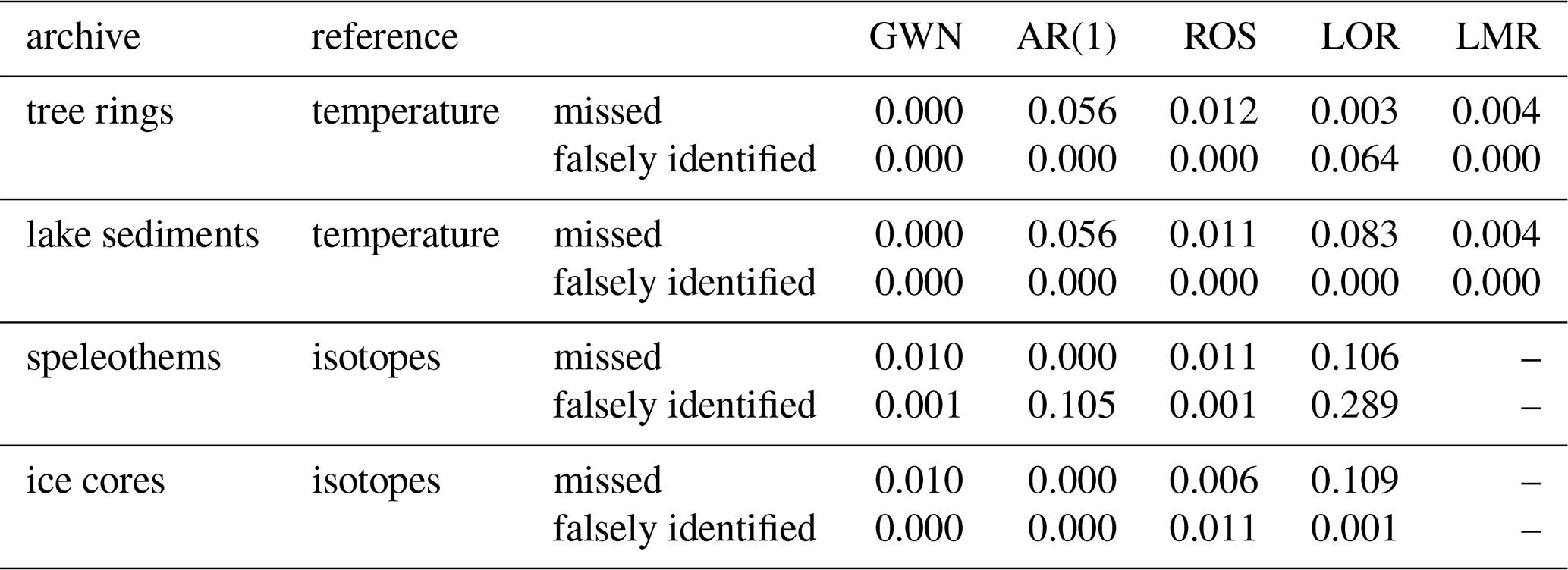
In order to quantify the effect of the proxy system models as non-linear filters of the input signal on the detection of areawise significant points, Table 5 displays the fraction of falsely identified and missed significant points in the different proxy models for the different input time series. We observe that for the tree ring width model, the lacustrine sediment model, and the ice core model missed significant points are more common than falsely identified significant points, with the exception of the Lorenz input for the tree ring width model. For the speleothem model, both falsely identified and missed significant points occur. In fact, this model shows particularly high fractions of falsely identified and missed significant points, while overall, the ice core model seems to best reproduce the results of the input in terms of the classification of areawise significant points.
Taken together, the previous findings should raise awareness in the context of future applications of wRNA to palaeoclimate proxy time series, suggesting that interpretations of results obtained for individual records only may not be sufficiently robust for drawing substantiated conclusions. From a practical perspective, this calls for combining different time series from different proxies and/or archives from the same region to obtain further climatological knowledge from such kinds of analysis (Donges et al., 2015a; Franke and Donner, 2017).
In this paper, we have studied the suitability of windowed recurrence network analysis (wRNA) for detecting dynamical anomalies in time series from different proxy archives. For this, we used proxy system models that simulate the formation of proxy archives, such as tree rings, lake sediments, speleothems, and ice cores, given some climatic input variables like temperature and precipitation. We created artificial input time series with different properties and additionally used temperature and precipitation data from the Last Millennium Reanalysis project (Hakim et al., 2016; Tardif et al., 2019). We then processed the input time series through the different proxy models and contrasted the results of wRNA for the different input and model output time series.
We first compared the results of wRNA for stochastic and deterministic input to corresponding results when filtering the time series using moving average filtering and exponential smoothing (results not shown). We found that filtering alters the variability of the network transitivity, with a bias towards additional and extended patches of areawise significant high transitivity values for stochastic input. The network transitivity of deterministic input seems to be rather robust under such filtering. When processing the input time series through the different proxy system models, these differences for stochastic and deterministic input were also apparent. In terms of areawise significant anomalies of the network transitivity, we found that time series of tree ring width and brGDGTs in lake sediments have problems with missing areawise significant points, while the isotopic composition of speleothems also exhibits falsely identified significant points of high values of the network transitivity probably related to the bias towards higher values of the network transitivity due to the particular filtering in the model. Time series of the isotopic composition of ice yield comparable results to the corresponding input, but also sometimes miss significant points.
Taken together, our results show the need for further study of the effects of different filtering mechanisms on the results of the wRNA in order to interpret the results and draw reliable conclusions when analysing real-world data. This particularly concerns data from speleothems, as they have been studied quite often using windowed recurrence analysis (e.g. Donges et al., 2015a; Eroglu et al., 2016), and filtering effects seem to have a non-negligible influence on the results for this type of archive. Thus, the role of the model parameters that control the filtering (here, the mean aquifer transit time) should be studied in more detail and in the context of the real-world applications and should be taken into account for estimates of these parameters for the particular data to better interpret corresponding results of the network transitivity.
Still, we want to stress that even then, providing a general recipe for interpreting the resulting network transitivity is hardly possible in the (palaeo)climate context. Climate-related interpretations always vary depending on the location and, thus, local boundary conditions have to be taken into account. As motivated in Sect. 2, the network transitivity has been related to the dynamical regularity of the variations in the analysed time series (e.g. Donges et al., 2011b), with higher values of the network transitivity corresponding to less irregular variability and vice versa. This is in accordance with the interpretation of the network transitivity as an indicator of the dimensionality of the system's dynamics. In this regard, detected anomalies in the network transitivity could be related to some tipping point, but do not have to be.
Future work should also include the study of alternative proxy system models within this framework. Results of proxy system models for both the same proxies (but with more detailed systemic understanding of the formation of the proxies, as for example a tree ring width model accounting for juvenile growth of the trees) and different proxy variables (in particular, for other lacustrine proxy variables) will complement the improved understanding of the suitability of wRNA for these types of time series and will advance the interpretation of the corresponding results. Also, sensitivity studies for the different model parameters are of interest to better interpret results obtained with wRNA for a given real-world data set. This concerns particularly the mean aquifer transit time of the speleothem model.
For the stochastic input time series as for example the isotope input of GWN, we found some areawise significant artefacts in single realisations. To improve the reliability of the results for the these processes, more realisations should be considered to confirm the results and to exclude the influence of random artefacts. As we applied an areawise significance test to identify dynamical anomalies, which reduces the number of false positives in the analysis results, this can also reduce the number of true positives and increase the number of false negatives independent of whether considering model input or output time series. In this regard, we also observed that time series with stronger autocorrelations in most cases show higher correlations for the wRNA results in the different domains and, thus, have more restrictive bounds of the areawise significance test (not shown).
Additionally, the study of properties of the analysed time series can serve as a starting point to judge the suitability of wRNA for other data to be analysed. In particular, the effect of filtering the time series with different non-linear filters prior to the analysis as done within the different proxy system models can and should be studied more systematically. Also, the theory of non-linear observability might give an interesting new perspective on this as the filtering can be seen as creating a new observable, and the choice of observable has already been shown to influence results of recurrence quantification analysis and recurrence network analysis (Portes et al., 2014, 2019). Moreover, further systematically studying the relation between the autocorrelation of a time series and the resulting network properties might yield additional information on the role of the different archives for the results of wRNA.
Exemplary Python code for the windowed recurrence network analysis including the areawise significance test is available at https://gitlab.pik-potsdam.de/lekscha/awsig (last access: 12 March 2019).
A comprehensive implementation of recurrence network analysis can be found in the pyunicorn open-source Python package (Donges et al., 2015b), which can be found at https://github.com/pik-copan/pyunicorn (last access: 10 November 2017).
The supplement related to this article is available online at: https://doi.org/10.5194/npg-27-261-2020-supplement.
JL and RVD designed the research. JL performed the numerical experiments and data analyses. JL and RVD discussed the results and wrote the manuscript.
The authors declare that they have no conflict of interest.
Calculations have been performed with the help
of the pyunicorn Python package (Donges et al., 2015b).
This research has been supported by the Bundesministerium für Bildung und Forschung (BMBF) via the BMBF Young Investigators Group, CoSy-CC2 – Complex Systems Approaches to Understanding Causes and Consequences of Past, Present and Future Climate Change (grant no. 01LN1306A) and the Studienstiftung des Deutschen Volkes.
The publication of this article was funded by the
Open Access Fund of the Leibniz Association.
This paper was edited by Stéphane Vannitsem and reviewed by Dmitry Divine and Michel Crucifix.
Abarbanel, H. D. I., Brown, R., Sidorowich, J. J., and Tsimring, L. S.: The analysis of observed chaotic data in physical systems, Rev. Mod. Phys., 65, 1331–1392, https://doi.org/10.1103/revmodphys.65.1331, 1993. a
Barrio, R. and Serrano, S.: A three-parametric study of the Lorenz model, Physica D, 229, 43–51, https://doi.org/10.1016/j.physd.2007.03.013, 2007. a
Bradley, R. S.: Paleoclimatology (Third Edition), Academic Press, third edition edn., https://doi.org/10.1016/C2009-0-18310-1, 2015. a, b
Cohen, A.: Paleolimnology: The History and Evolution of Lake Systems, Oxford University Press, 2003. a
Dee, S., Emile-Geay, J., Evans, M. N., Allam, A., Steig, E. J., and Thompson, D.: PRYSM: An open-source framework for PRoxY System Modeling, with applications to oxygen-isotope systems, J. Adv. Model. Earth Sy., 7, 1220–1247, https://doi.org/10.1002/2015MS000447, 2015. a, b, c
Dee, S. G., Russell, J. M., Morrill, C., Chen, Z., and Neary, A.: PRYSM v2.0: A Proxy System Model for Lacustrine Archives, Paleoceanogr. Paleocl., 33, 1250–1269, https://doi.org/10.1029/2018PA003413, 2018. a, b, c
De Jonge, C., Hopmans, E. C., Zell, C. I., Kim, J.-H., Schouten, S., and Damsté, J. S. S.: Occurrence and abundance of 6-methyl branched glycerol dialkyl glycerol tetraethers in soils: Implications for palaeoclimate reconstruction, Geochim. Cosmochim. Ac., 141, 97–112, https://doi.org/10.1016/j.gca.2014.06.013, 2014. a
Donges, J. F., Donner, R. V., Rehfeld, K., Marwan, N., Trauth, M. H., and Kurths, J.: Identification of dynamical transitions in marine palaeoclimate records by recurrence network analysis, Nonlin. Processes Geophys., 18, 545–562, https://doi.org/10.5194/npg-18-545-2011, 2011a. a, b, c, d
Donges, J. F., Donner, R. V., Trauth, M. H., Marwan, N., Schellnhuber, H.-J., and Kurths, J.: Nonlinear detection of paleoclimate-variability transitions possibly related to human evolution, P. Natl. Acad. Sci. USA, 108, 20422–20427, https://doi.org/10.1073/pnas.1117052108, 2011b. a, b
Donges, J. F., Donner, R. V., Marwan, N., Breitenbach, S. F. M., Rehfeld, K., and Kurths, J.: Non-linear regime shifts in Holocene Asian monsoon variability: potential impacts on cultural change and migratory patterns, Clim. Past, 11, 709–741, https://doi.org/10.5194/cp-11-709-2015, 2015a. a, b
Donges, J. F., Heitzig, J., Beronov, B., Wiedermann, M., Runge, J., Feng, Q. Y., Tupikina, L., Stolbova, V., Donner, R. V., Marwan, N., Dijkstra, H. A., and Kurths, J.: Unified functional network and nonlinear time series analysis for complex systems science: The pyunicorn package, Chaos, 25, 113101, https://doi.org/10.1063/1.4934554, 2015b. a, b
Donner, R. V., Zou, Y., Donges, J. F., Marwan, N., and Kurths, J.: Ambiguities in recurrence-based complex network representations of time series, Phys. Rev. E, 81, 015101, https://doi.org/10.1103/physreve.81.015101, 2010a. a
Donner, R. V., Zou, Y., Donges, J. F., Marwan, N., and Kurths, J.: Recurrence networks – a novel paradigm for nonlinear time series analysis, New J. Phys., 12, 033025, https://doi.org/10.1088/1367-2630/12/3/033025, 2010b. a
Donner, R. V., Heitzig, J., Donges, J. F., Zou, Y., Marwan, N., and Kurths, J.: The geometry of chaotic dynamics – a complex network perspective, Eur. Phys. J. B, 84, 653–672, https://doi.org/10.1140/epjb/e2011-10899-1, 2011a. a, b
Donner, R. V., Small, M., Donges, J. F., Marwan, N., Zou, Y., Xiang, R., and Kurths, J.: Recurrence-based time series analysis by means of complex network methods, Int. J. Bifurcat. Chaos, 21, 1019–1046, https://doi.org/10.1142/s0218127411029021, 2011b. a
Eroglu, D., McRobie, F. H., Ozken, I., Stemler, T., Wyrwoll, K.-H., Breitenbach, S. F. M., Marwan, N., and Kurths, J.: See-saw relationship of the Holocene East Asian-Australian summer monsoon, Nat. Commun., 7, 12929, https://doi.org/10.1038/ncomms12929, 2016. a, b
Esper, J., Krusic, P. J., Ljungqvist, F. C., Luterbacher, J., Carrer, M., Cook, E., Davi, N. K., Hartl-Meier, C., Kirdyanov, A., Konter, O., Myglan, V., Timonen, M., Treydte, K., Trouet, V., Villalba, R., Yang, B., and Büntgen, U.: Ranking of tree-ring based temperature reconstructions of the past millennium, Quaternary Sci. Rev., 145, 134–151, https://doi.org/10.1016/j.quascirev.2016.05.009, 2016. a
Evans, M., Tolwinski-Ward, S., Thompson, D., and Anchukaitis, K.: Applications of proxy system modeling in high resolution paleoclimatology, Quaternary Sci. Rev., 76, 16–28, https://doi.org/10.1016/j.quascirev.2013.05.024, 2013. a, b
Franke, J. G. and Donner, R. V.: Dynamical anomalies in terrestrial proxies of North Atlantic climate variability during the last 2 ka, Climatic Change, 143, 87–100, https://doi.org/10.1007/s10584-017-1979-z, 2017. a, b, c, d
Fraser, A. M. and Swinney, H. L.: Independent coordinates for strange attractors from mutual information, Phys. Rev. A, 33, 1134–1140, https://doi.org/10.1103/PhysRevA.33.1134, 1986. a
Fritts, H. C.: Tree rings and climate, Academic Press, https://doi.org/10.1016/B978-0-12-268450-0.X5001-0, 1976. a
Gennaretti, F., Arseneault, D., Nicault, A., Perreault, L., and Bégin, Y.: Volcano-induced regime shifts in millennial tree-ring chronologies from northeastern North America, P. Natl. Acad. Sci. USA, 111, 10077–10082, https://doi.org/10.1073/pnas.1324220111, 2014. a, b, c, d
Goswami, B., Boers, N., Rheinwalt, A., Marwan, N., Heitzig, J., Breitenbach, S. F. M., and Kurths, J.: Abrupt transitions in time series with uncertainties, Nat. Commun., 9, 48, https://doi.org/10.1038/s41467-017-02456-6, 2018. a
Hakim, G. J., Emile-Geay, J., Steig, E. J., Noone, D., Anderson, D. M., Tardif, R., Steiger, N., and Perkins, W. A.: The last millennium climate reanalysis project: Framework and first results, J. Geophys. Res.-Atmos., 121, 6745–6764, https://doi.org/10.1002/2016JD024751, 2016. a, b, c, d
Herron, M. M. and Langway, C. C.: Firn Densification: An Empirical Model, J. Glaciol., 25, 373–385, https://doi.org/10.3189/S0022143000015239, 1980. a
Huang, J., van den Dool, H. M., and Georgarakos, K. P.: Analysis of Model-Calculated Soil Moisture over the United States (1931–1993) and Applications to Long-Range Temperature Forecasts, J. Climate, 9, 1350–1362, https://doi.org/10.1175/1520-0442(1996)009<1350:AOMCSM>2.0.CO;2, 1996. a
Johnsen, S. J., Clausen, H. B., Cuffey, K. M., Hoffmann, G., Schwander, J., and Creyts, T.: Diffusion of stable isotopes in polar firn and ice: the isotope effect in firn diffusion, Physics of Ice Core Records, 159, 121–140, https://doi.org/10.7916/D8KW5D4X, 2000. a
ouzel, J.: A brief history of ice core science over the last 50 yr, Clim. Past, 9, 2525–2547, https://doi.org/10.5194/cp-9-2525-2013, 2013. a
Kantz, H. and Schreiber, T.: Nonlinear time series analysis, Cambridge University Press, 2 edn., 2004. a
Kennel, M. B., Brown, R., and Abarbanel, H. D. I.: Determining embedding dimension for phase-space reconstruction using a geometrical construction, Phys. Rev. A, 45, 3403–3411, https://doi.org/10.1103/PhysRevA.45.3403, 1992. a
Lekscha, J. and Donner, R. V.: Phase space reconstruction for non-uniformly sampled noisy time series, Chaos, 28, 085702, https://doi.org/10.1063/1.5023860, 2018. a, b
Lekscha, J. and Donner, R. V.: Areawise significance tests for windowed recurrence network analysis, P. Roy. Soc. A, 475, 20190161, https://doi.org/10.1098/rspa.2019.0161, 2019. a, b, c
Lorenz, E. N.: Deterministic Nonperiodic Flow, J. Atmos. Sci., 20, 130–141, https://doi.org/10.1175/1520-0469(1963)020<0130:dnf>2.0.co;2, 1963. a, b
Maraun, D., Kurths, J., and Holschneider, M.: Nonstationary Gaussian processes in wavelet domain: Synthesis, estimation, and significance testing, Phys. Rev. E, 75, 016707, https://doi.org/10.1103/PhysRevE.75.016707, 2007. a
Marwan, N., Thiel, M., and Nowaczyk, N. R.: Cross recurrence plot based synchronization of time series, Nonlin. Processes Geophys., 9, 325–331, https://doi.org/10.5194/npg-9-325-2002, 2002. a
Marwan, N., Trauth, M. H., Vuille, M., and Kurths, J.: Comparing modern and Pleistocene ENSO-like influences in NW Argentina using nonlinear time series analysis methods, Clim. Dynam., 21, 317–326, https://doi.org/10.1007/s00382-003-0335-3, 2003. a
Marwan, N., Donges, J. F., Zou, Y., Donner, R. V., and Kurths, J.: Complex network approach for recurrence analysis of time series, Phys. Lett. A, 373, 4246–4254, https://doi.org/10.1016/j.physleta.2009.09.042, 2009. a
Packard, N. H., Crutchfield, J. P., Farmer, J. D., and Shaw, R. S.: Geometry from a Time Series, Phys. Rev. Lett., 45, 712–716, https://doi.org/10.1103/physrevlett.45.712, 1980. a
Partin, J. W., Quinn, T. M., Shen, C.-C., Emile-Geay, J., Taylor, F. W., Maupin, C. R., Lin, K., Jackson, C. S., Banner, J. L., Sinclair, D. J., and Huh, C.-A.: Multidecadal rainfall variability in South Pacific Convergence Zone as revealed by stalagmite geochemistry, Geology, 41, 1143–1146, https://doi.org/10.1130/G34718.1, 2013. a
Portes, L. L., Benda, R. N., Ugrinowitsch, H., and Aguirre, L. A.: Impact of the recorded variable on recurrence quantification analysis of flows, Phys. Lett. A, 378, 2382–2388, https://doi.org/10.1016/j.physleta.2014.06.014, 2014. a
Portes, L. L., Montanari, A. N., Correa, D. C., Small, M., and Aguirre, L. A.: The reliability of recurrence network analysis is influenced by the observability properties of the recorded time series, Chaos, 29, 083101, https://doi.org/10.1063/1.5093197, 2019. a
Rössler, O.: An equation for continuous chaos, Phys. Lett. A, 57, 397–398, https://doi.org/10.1016/0375-9601(76)90101-8, 1976. a
Russell, J. M., Hopmans, E. C., Loomis, S. E., Liang, J., and Damsté, J. S. S.: Distributions of 5- and 6-methyl branched glycerol dialkyl glycerol tetraethers (brGDGTs) in East African lake sediment: Effects of temperature, pH, and new lacustrine paleotemperature calibrations, Org. Geochem., 117, 56–69, https://doi.org/10.1016/j.orggeochem.2017.12.003, 2018. a, b
Schleussner, C.-F., Divine, D. V., Donges, J. F., Miettinen, A., and Donner, R. V.: Indications for a North Atlantic ocean circulation regime shift at the onset of the Little Ice Age, Clim. Dynam., 45, 3623–3633, https://doi.org/10.1007/s00382-015-2561-x, 2015. a
Schreiber, T. and Schmitz, A.: Surrogate time series, Physica D, 142, 346–382, https://doi.org/10.1016/S0167-2789(00)00043-9, 2000. a
St. George, S.: An overview of tree-ring width records across the Northern Hemisphere, Quaternary Sci. Rev., 95, 132–150, https://doi.org/10.1016/j.quascirev.2014.04.029, 2014. a
St. George, S. and Esper, J.: Concord and discord among Northern Hemisphere paleotemperature reconstructions from tree rings, Quaternary Sci. Rev., 203, 278–281, https://doi.org/10.1016/j.quascirev.2018.11.013, 2019. a
Takens, F.: Detecting strange attractors in turbulence, in: Lecture Notes in Mathematics, 366–381, Springer Science and Business Media, https://doi.org/10.1007/bfb0091924, 1980. a, b
Tardif, R., Hakim, G. J., Perkins, W. A., Horlick, K. A., Erb, M. P., Emile-Geay, J., Anderson, D. M., Steig, E. J., and Noone, D.: Last Millennium Reanalysis with an expanded proxy database and seasonal proxy modeling, Clim. Past, 15, 1251–1273, https://doi.org/10.5194/cp-15-1251-2019, 2019. a, b, c, d
Thompson, L. G., Davis, M. E., Mosley-Thompson, E., Lin, P.-N., Henderson, K. A., and Mashiotta, T. A.: Tropical ice core records: evidence for asynchronous glaciation on Milankovitch timescales, J. Quaternary Sci., 20, 723–733, https://doi.org/10.1002/jqs.972, 2005. a
Thompson, L. G., Mosley-Thompson, E., Davis, M. E., Zagorodnov, V. S., Howat, I. M., Mikhalenko, V. N., and Lin, P.-N.: Annually Resolved Ice Core Records of Tropical Climate Variability over the Past ∼1800 Years, Science, 340, 945–950, https://doi.org/10.1126/science.1234210, 2013. a, b
Tolwinski-Ward, S. E., Evans, M. N., Hughes, M. K., and Anchukaitis, K. J.: An efficient forward model of the climate controls on interannual variation in tree-ring width, Clim. Dynam., 36, 2419–2439, https://doi.org/10.1007/s00382-010-0945-5, 2011. a, b, c
Tolwinski-Ward, S. E., Anchukaitis, K. J., and Evans, M. N.: Bayesian parameter estimation and interpretation for an intermediate model of tree-ring width, Clim. Past, 9, 1481–1493, https://doi.org/10.5194/cp-9-1481-2013, 2013. a
Trauth, M. H.: TURBO2: A MATLAB simulation to study the effects of bioturbation on paleoceanographic time series, Comput. Geosci., 61, 1–10, https://doi.org/10.1016/j.cageo.2013.05.003, 2013. a
Trauth, M. H., Bookhagen, B., Marwan, N., and Strecker, M. R.: Multiple landslide clusters record Quaternary climate changes in the northwestern Argentine Andes, Palaeogeogr. Palaeocl., 194, 109–121, https://doi.org/10.1016/s0031-0182(03)00273-6, 2003. a
Vaganov, E. A., Hughes, M. K., and Shashkin, A. V.: Growth Dynamics of Conifer Tree Rings, Springer-Verlag Berlin Heidelberg, 1 edn., https://doi.org/10.1007/3-540-31298-6, 2006. a
Wackerbarth, A., Scholz, D., Fohlmeister, J., and Mangini, A.: Modelling the δ18O value of cave drip water and speleothem calcite, Earth Planet. Sc. Lett., 299, 387–397, https://doi.org/10.1016/j.epsl.2010.09.019, 2010. a
Wang, Y., Cheng, H., Edwards, R. L., He, Y., Kong, X., An, Z., Wu, J., Kelly, M. J., Dykoski, C. A., and Li, X.: The Holocene Asian Monsoon: Links to Solar Changes and North Atlantic Climate, Science, 308, 854–857, https://doi.org/10.1126/science.1106296, 2005. a, b
Weijers, J. W., Schouten, S., van den Donker, J. C., Hopmans, E. C., and Damsté, J. S. S.: Environmental controls on bacterial tetraether membrane lipid distribution in soils, Geochim. Cosmochim. Ac., 71, 703–713, https://doi.org/10.1016/j.gca.2006.10.003, 2007. a
Wong, C. I. and Breecker, D. O.: Advancements in the use of speleothems as climate archives, Quaternary Sci. Rev., 127, 1–18, https://doi.org/10.1016/j.quascirev.2015.07.019, 2015. a
Yarleque, C., Vuille, M., Hardy, D. R., Timm, O. E., De la Cruz, J., Ramos, H., and Rabatel, A.: Projections of the future disappearance of the Quelccaya Ice Cap in the Central Andes, Sci. Rep.-UK, 8, 15564–15564, https://doi.org/10.1038/s41598-018-33698-z, 2018. a, b
Zumbahlen, H.: CHAPTER 8 – Analog Filters, in: Linear Circuit Design Handbook, edited by: Zumbahlen, H., Newnes, https://doi.org/10.1016/B978-0-7506-8703-4.00008-0, 2008. a