Prediction and variation of the auroral oval boundary based on a deep learning model and space physical parameters

The auroral oval boundary represents an important physical process with implications for the ionosphere and magnetosphere. An automatic auroral oval boundary prediction method based on deep learning in this paper is applied to study the variation of the auroral oval boundary associated with different space physical parameters. We construct an auroral oval boundary dataset to train our proposed model, which consists of 184 416 auroral oval boundary points extracted from 3842 images captured by the Ultraviolet Imager (UVI) of the Polar satellite and its corresponding 18 space physical parameters selected from the OMNI dataset from December 1996 to March 1997. Furthermore, several statistical experiments and correlation analysis experiments are performed based on our dataset to explore the relationship between space physical parameters and the location of the auroral oval boundary. The experiment results show that the prediction model based on the deep learning method can estimate the auroral oval boundary efficiently, and different space physical parameters have different effects on the auroral oval boundary, especially the interplanetary magnetic field (IMF), geomagnetic indexes, and solar wind parameters.

1 Introduction

An auroral oval is a circular belt of auroral emission around magnetic poles (Loomis, 1890; Akasofu, 1964). The auroral oval poleward and equatorward boundaries are related to geophysical parameters, which can indicate for the coupling process among the solar wind, ionosphere, and magnetosphere, for example, the polar cap ionosphere, which is considered an area of the opening magnetic field inside the auroral oval poleward boundary. This area is closely related to energetic particle entrance from the heliosphere to the earth's atmosphere. So, the segmentation and prediction for the auroral oval boundary are very significant for studying certain physical events.

In the past few decades, scholars have conducted extensive research on the relationship between the location of the auroral oval boundary and space physical parameters (Niu et al., 2015). In early research, Feldstein proposed that the position of the auroral oval boundary is correlated with the Q index of magnetic activity on the nightside of the earth (Feldstein and Starkov, 1967). Starkov and Holzworth stated that the inner and outer boundaries of the auroral oval can change with geomagnetic indexes and the interplanetary magnetic field (IMF) (Holzworth and Meng, 1975; Holzworth and Meng, 1984; Starkov, 1994a). The conclusions in this paper are based on mathematical statistics. Therefore, Starkov designed some simple formulas to describe the relationships between the specific physical parameter and different types of auroras. Variations of the sizes of the polar cap, auroral oval, and diffuse aurora were regarded as three independent function variables of the AL index (Starkov, 1994b). Since then, many scholars have explored the connections between different physical parameters and the auroral oval boundary or other auroral events. Carbary constructed a Kp-related model of the auroral oval boundary by binning Ultraviolet Imager (UVI) images from different months (Carbary, 2005). To describe the particle precipitation characteristics, Zhang and Paxton proposed a Kp-dependent model of the mean energy and energy flux precipitating electrons in the auroral oval (Zhang and Paxton, 2008). Sigernes et al. used a Kp-based function to calculate the size and position of the auroral oval and compared the Kp-dependent model with methods proposed by Zhang and Starkov to explain the superiority of his proposed model (Sigernes et al., 2011). Milan proposed a model based on average protons and electrons of auroral images from 3 years observed by the IMAGE spacecraft. The experiment demonstrated that Kp, solar wind parameters including solar wind velocity, density, and pressure, IMF magnitude, and orientation have an effect on the intensity and shape of the auroral oval (Milan, 2010). Since 2010, there have been more and more new methods to construct a connection between the position of the auroral oval boundary and space physical parameters with the development of machine learning. Hu and Yang used the segmentation results of the auroral oval obtained from the UVI on the Polar satellite to build a connection between the positions of the auroral oval boundary and the auroral electrojet (AE) index, the IMF, and solar wind parameters by using a multiple regression method (Hu et al., 2017; Yang et al., 2016). Ding presented a C-means clustering algorithm based on fuzzy local information to extract the auroral oval poleward and equatorward boundaries from merged images with filled gaps captured from both GUVI and SSUSI (Ding et al., 2017). However, the position of the auroral oval boundary is not determined by one space physical parameter; those methods mentioned above only used one or several space physical parameters to explore the relationship between space physical parameters and the auroral oval boundary. We cannot determine whether other space physical parameters can influence the location or size of the auroral oval, and we also do not know whether the mapping relationship between space physical parameters and the auroral oval boundary is linear or non-linear.

As we know, machine learning has been applied to many fields, including the medical, traffic, space physics, and other interdisciplinary fields. Recently, deep learning models have led to a series of breakthroughs in image classification, object detection, image recognition, and other fields. Conventional machine learning methods have some limitations for processing complex data, especially in the space physics field. There are no suitable internal features, such as shape and colour. Therefore, many effective machine learning methods cannot obtain satisfactory performance on processing space physics data, while deep learning methods are representation learning methods with multiple levels of representation. They have turned out to be very good at discovering intricate structures in high-dimensional data and multimodal data (LeCun et al., 2015).

In this paper, a new automatic auroral oval boundary prediction model is proposed based on a deep learning method. The experiment results show that the model proposed in this paper can predict the auroral oval boundary accurately by using space physical parameters and the location of the auroral oval boundary at the previous moment. In addition, we explore the effect of every space physical parameter on the auroral oval boundary. The rest of this paper is organized as follows. Section 2 describes our proposed algorithm in detail. The experiment analysis and discussion are given in Sect. 3, including dataset construction, subjective and objective evaluation, the selection of model parameters, and the discussion about the influence of every space physical parameter on the auroral oval boundary. Finally, we draw several conclusions in Sect. 4.

Figure 1 The flowchart of the auroral oval boundary prediction model based on deep learning.

2 Prediction of the auroral oval boundary based on the deep learning method

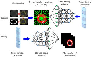
The flowchart of the auroral oval boundary prediction model is shown in Fig. 1. There are two major steps in our proposed model, pre-training on our dataset and online prediction. In the training phase, auroral oval images are usually affected by heavy noise and other interferences. So, the auroral oval boundary is blurred, and it is difficult to find from the background. Compared with other image segmentation methods, maximal similarity-based region merging (MRSM) (Liu et al., 2013) can eliminate the cumbersome process of adjusting parameters and has better segmentation accuracy. We use MRSM firstly to extract positions of the auroral oval boundary. The centre of the auroral oval spatial distribution in the magnetic local time–magnetic latitude coordinate (MLT–MLAT) is located in the geomagnetic pole. The magnetic latitude of the auroral oval usually ranged from 57.5 to 73.5^∘ according to the statistical studies on previous work (King and Papitashvili, 2014). In order to unify the distribution of the auroral oval boundary, the coordinates of those extracted boundary points are transformed into the MLT–MLAT coordinate secondly. Finally, these transformed boundary points and their corresponding space physical parameters were input into the deep learning network to train our prediction model. In the testing phase, we can obtain the corresponding boundary points of the auroral oval by sending those space physical parameters and the positions of auroral oval boundary points at the previous moment to our well-trained network.

The deep learning network is constructed by a two-layer restricted Boltzmann machine (RBM) network (Hinton et al., 2006; Yu and Deng, 2011) and a radial basis function (RBF) network (Łukaszyk, 2004). The computational processing of the RBM and RBF is illustrated by Eqs. (1)–(4). In the training phase, the inputs of the RBM network are 18 space physical parameters from the OMNI dataset and coordinate values of the auroral oval poleward and equatorward boundaries extracted from segmented UVI images with MRSM. They can be represented as $X=[x_{\mathrm{1}}{x}_{\mathrm{2}},\mathrm{\dots },x_m{]}^T$, where m is the number of network nodes. The first layer of the RBM network is denoted as ${\mathit{\theta }}_{\mathrm{1}}=\left\{w_{i_{\mathrm{1}}{j}_{\mathrm{1}}},a_{i_{\mathrm{1}}},b_{j_{\mathrm{1}}}\right\}$, where $w_{i_{\mathrm{1}}{j}_{\mathrm{1}}}$ is the weight between the visible unit i₁ and the hidden unit j₁, $a_{i_{\mathrm{1}}}$ is the bias of the visible unit i₁, and $b_{j_{\mathrm{1}}}$ is the bias of the hidden unit j₁. The hidden layer of the first layer in the RBM network is the visible layer of the second layer in the RBM network, which is denoted as ${\mathit{\theta }}_{\mathrm{2}}=\left\{w_{j_{\mathrm{1}}{j}_{\mathrm{2}}},a_{j_{\mathrm{1}}},b_{j_{\mathrm{2}}}\right\}$, where $w_{j_{\mathrm{1}}{j}_{\mathrm{2}}}$ is the weight between the visible unit j₁ and the hidden unit j₂, $a_{j_{\mathrm{1}}}$ is the bias of the visible unit j₁, and $b_{j_{\mathrm{2}}}$ is the bias of the hidden unit j₂. The output of the first layer of the RBM network is denoted as $Y_{\mathrm{1}}=[y_{\mathrm{11},}{y}_{\mathrm{12}}\mathrm{\dots }{y}_{\mathrm{1}n}{]}^T$, where n denotes the node number of the first layer in the RBM network.

$$\begin{array}{}\text{(1)}& y_{\mathrm{1}{j}_{\mathrm{1}}}={\sum }_{i=\mathrm{1}}^m{x}_{i_{\mathrm{1}}}{w}_{i_{\mathrm{1}}{j}_{\mathrm{1}}}+b_{j_{\mathrm{1}}}{j}_{\mathrm{1}}=\mathrm{1},\mathrm{2},\mathrm{\dots }n\end{array}$$

The output of the second layer of the RBM network is denoted as $Y_{\mathrm{2}}={\left[y_{\mathrm{21}},y_{\mathrm{22}},\mathrm{\dots },y_{\mathrm{2}c}\right]}^T$, where c denotes the node number of the second layer in the RBM network.

$$\begin{array}{}\text{(2)}& y_{\mathrm{2}{j}_{\mathrm{2}}}={\sum }_{j=\mathrm{1}}^n{x}_{j_{\mathrm{1}}}{w}_{j_{\mathrm{1}}{j}_{\mathrm{2}}}+b_{j_{\mathrm{2}}}{j}_{\mathrm{2}}=\mathrm{1},\mathrm{2},\mathrm{\dots }c\end{array}$$

Finally, since contrastive divergence (CD) (Hinton, 2002) is an approximation of the log-likelihood gradient which has been found to be a successful update rule for training an RBM, we can obtain a well-trained RBM network by CD.

The function of the RBF network can make the output of the RBM network infinitely approximate to the coordinate values of the auroral oval boundary by a radial basis function. The input of the RBF network is the output of the second layer in the RBM network. The output of the RBF network is represented as $Y={\left[y_{\mathrm{1}},y_{\mathrm{2}},\mathrm{\dots },y_d\right]}^T$, where d denotes the number of the output layer nodes. $w_{j_{\mathrm{3}o}}$ is the weight between the hidden unit j₃ and the output node o. l is the number of the radial basis function. ${\mathit{\phi }}_{j_{\mathrm{3}}}$ is the jth radial basis function and $c_{j_{\mathrm{3}}}$ is the centre of the jth radial basis function. ${\mathit{\sigma }}_{j_{\mathrm{3}}}$ is the centre width of the radial basis function.

$$\begin{array}{}\text{(3)}& {\displaystyle }{y}_o={\sum }_{j_{\mathrm{3}}=\mathrm{1}}^l{w}_{j_{\mathrm{3}o}}{\mathit{\phi }}_{j_{\mathrm{3}}}\left(\right||Y_{\mathrm{2}}-c_{j_{\mathrm{3}}}|\left|\right)o=\mathrm{1},\mathrm{2},\mathrm{\dots }d\text{(4)}& {\displaystyle }{\mathit{\phi }}_{j_{\mathrm{3}}}\left(\right||Y_{\mathrm{2}}-c_{j_{\mathrm{3}}}|\left|\right)=\exp (-{\displaystyle \frac{\left|\right|Y_{\mathrm{2}}-c_{j_{\mathrm{3}}}|{|}^{\mathrm{2}}}{{\mathit{\sigma }}_{j_{\mathrm{3}}}^{\mathrm{2}}}})j_{\mathrm{3}}=\mathrm{1},\mathrm{2},\mathrm{\dots }l\end{array}$$

3 Experiments and results analysis

3.1 Dataset construction and evaluation criteria

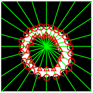
The auroral oval images used in this paper are captured by the UVI, which is a 2-D snapshot-type camera on the Polar satellite. The UVI on the Polar satellite acquired more than several million images during its entire mission. As of April 2008, it is no longer active. There was no effective observation after 2000, because the Polar satellite changed its view after 2000. In order to balance the relationship between spatial resolution and global coverage, the spatial resolution of the UVI is 30 km at apogee, the charge-coupled device (CCD) array onboard has 224×220 pixels, and the single-pixel spatial resolution is 0.0036 and 0.04^∘ in the two directions respectively. The unilluminated edges of CCD are discarded, which results in the frame size of an auroral oval image being 200 by 228 pixels and the frame rate being 37 s. There are four band sensors aboard the satellite usually. UVI images in our dataset are derived from a Lyman–Brige–Hopfield long band (160–180 mm). In our experiments, each auroral oval image is divided into 24 magnetic regions centered on the geomagnetic pole according to magnetic local time (MLT). As shown in Fig. 2, the intersection points between the auroral oval boundary and division line are extracted. We extracted 48 boundary points from one auroral oval image. The poleward and equatorward boundary points are marked as a red triangle and a red circle respectively.

Figure 2 The schematic of extracting auroral boundary points.

Table 1 Space physical parameters selected from the OMNI dataset.

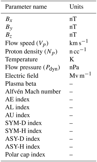
The space physical parameters were downloaded from the NASA OMNI dataset with a different time resolution. It is common knowledge that the IMF, solar wind parameters, and geomagnetic indexes have a time resolution of 1 min, and the other space physical parameters maybe have a higher time resolution. According to the effect derived from other circumstantial factors, such as the time to traverse the magnetosphere and Alfven wave, not all the response times of auroral events are equal to their propagation time. We align the time of all space physical parameters with the time of UVI images in our dataset to avoid the problem of different time resolution between space physical parameters and auroral oval images. In the OMNI dataset, we selected 18 space physical parameters, including the common parameters, which have been verified as being related to the position of the auroral oval boundary (Holzworth and Meng, 1975; Starkov, 1994a, b; Milan et al., 2010; Hu et al., 2017) and some unfamiliar parameters which are never discussed in previous works. Therefore, our dataset includes 184 416 auroral oval boundary points extracted from 3842 UVI images and its corresponding values of 18 space physical parameters. Table 1 shows the 18 space physical parameters which we used in this paper.

In order to evaluate the precision of predicted auroral oval boundary points by our model, we use the common metric MAE (mean absolute error) to assess the error between predicted auroral oval boundary points and real auroral oval boundary points. The MAE can be defined as Eq. (5).

$$\begin{array}{}\text{(5)}& \mathrm{MAE}={\displaystyle \frac{\mathrm{1}}{\mathrm{24}}}{\sum }_{i=\mathrm{1}}^{\mathrm{24}}\left({\displaystyle \frac{\mathrm{1}}{k}}{\sum }_{j=\mathrm{1}}^k|F_{\mathrm{MLAT}}^{ij}-S_{\mathrm{MLAT}}^{ij}|\right)\end{array}$$

$S_{\mathrm{MLAT}}^{ij}$ represents the MLAT of the j_th test sample at the j_th MLT region obtained from the segmented image, and $F_{\mathrm{MLAT}}^{ij}$ indicates the MLAT of the j_th test sample in the i_th MLT region acquired by our prediction model. k is the total number of test samples.

3.2 Parameter set-up of the deep learning network

Since the effectiveness of the prediction model is influenced by the number of hidden layer nodes in the RBM network (Hinton, 2012) and the training error of the RBF network, we build two experiments to find the most suitable parameters for our network. For both experiments, space physical parameters and positions of poleward and equatorward boundary points in 24 MLT regions of 3000 UVI images are selected as training samples, and the rest are regarded as test samples. In experiment 1, the training error of the RBF network is set to 4 magnetic latitudes and the numbers of hidden layer nodes in the RBM network are 32, 64, 96, and 128 respectively. We use the average MAE with 100 experiments to verify the stability of our model, because training samples and test samples were divided by a random number. The corresponding MAE is shown in Fig. 3a. From Fig. 3a, MAE reaches the smallest value when the number of hidden layer nodes is set to 32. In experiment 2, the number of hidden layer nodes is set to 32 according to the results in experiment 1. There often has been an overfitting problem when we train a neural network (Krizhevsky et al., 2012). Overfitting can be interpreted as a phenomenon where the model performs well on the training set and unsatisfactorily on the test set. We set different training errors to avoid the overfitting problem. So, the training error of the RBF network is set to 2, 4, 6, and 8 magnetic latitudes empirically. The corresponding MAE is shown in Fig. 3b, and MAE reaches the minimum when the training error of the RBF network is 4 magnetic latitudes. From the two experiment results above, we set the number of hidden layer nodes in the RBM network and the training error of the RBF network to 32 and 4 respectively as the optimal parameters of the deep learning network in the following experiments.

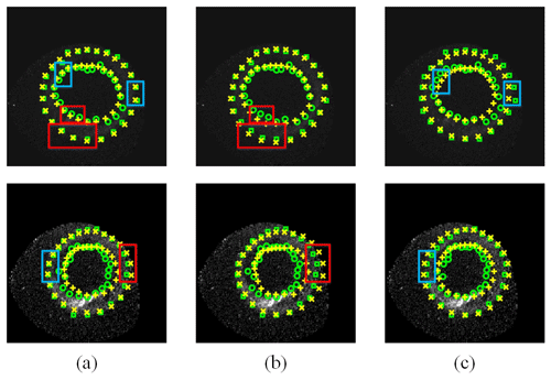
To demonstrate the availability of our proposed model, we compared the proposed model with a back-propagation (BP) network (Rumelhart, 1986) and Yang's model (Yang et al., 2016). The subjective prediction results obtained by the three methods are shown in Fig. 4; circles and squares stand for poleward boundary points and equatorward boundary points which are obtained from the segmented image, and “+” and “×” marks represent poleward boundary points and equatorward boundary points respectively which are obtained from our prediction model. Although these three methods have similar prediction results in most areas on the auroral oval boundary, it is obvious that our method can obtain more accurate boundaries than the other two compared methods, marked by blue rectangles and red rectangles in Fig. 4. In more detail, the results of the BP model and our model are shown in Fig. 4a and b respectively; we can clearly see that the distances between auroral oval boundary points predicted by our method and real auroral oval boundary points are smaller than the distances between the BP model's results and real auroral oval boundary points in red rectangle areas. From Fig. 4a and c, our prediction points are closer to real auroral oval boundary points compared with Yang's prediction points in blue rectangle areas. Meanwhile, the MAE values of different methods are shown in Table 2. From this table, our method has the smallest MAE not only on the poleward boundary, bur also on the equatorward boundary, because our model can extract more useful information and features from auroral oval images than the other two models. As a consequence, we can draw the conclusion that the proposed model in this paper is more suitable for predicting the auroral oval boundary.

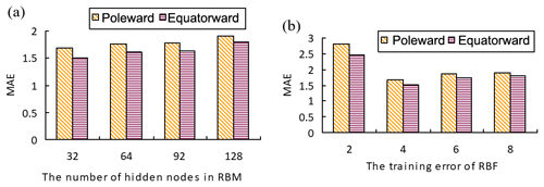
Figure 3 (a) The MAE values of the different hidden layer nodes. (b) The MAE values of the different training errors.

Figure 4 The different subjective results based on different methods. (a) The subjective results predicted by our method, (b) the subjective results predicted by the BP network, and (c) the subjective results predicted by the Yang et al. (2016) method.

Table 2 The MAE values of different methods.

3.3 The influence of space physical parameters on the auroral oval boundary

As we know, the location of the auroral oval boundary is affected by a variety of space physical parameters. Variations of the auroral oval boundary in different MLT sectors are related to different space physical parameters. For the sake of exploring the influence of space physical parameters on the poleward and equatorward boundaries specifically, the boundary points are further processed as follows (Hu et al., 2017). Firstly, all poleward and equatorward boundary points are divided into 24 subsets of poleward and equatorward boundary points according to 24 MLT sectors. Secondly, in every MLT subset, we sort boundary data with respect to the values of all the space physical parameters and divide boundary data into 10 groups evenly. In order to observe the variation tendency of each parameter in different MLT sectors clearly, in every MLT sector, the relationship between each space physical parameter and the location of the auroral oval boundary was represented as a quadratic equation based on the principles of the least square conic fitting (Fitzgibbon et al., 1999). Then, we calculate the locations of poleward and equatorward boundary points for each space physical parameter using this function. Finally, we use the boundary data calculated by the quadratic equation to discuss the influence of space physical parameters on the auroral oval boundary. In this section, we build three statistical experiments to discuss how the IMF, solar wind parameters, and geomagnetic indexes influence the auroral oval boundary, an auroral oval boundary prediction experiment by inputting every single space physical parameter to explore the relationship between the auroral oval boundary and 18 space physical parameters, and a correlation analysis experiment is constructed to study the connection between a combination of different space physical parameters and the auroral oval boundary.

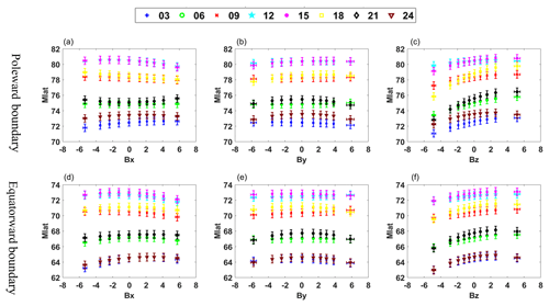
Figure 5 Responses of the magnetic latitudes of the poleward (a, b, c) and equatorward (d, e, f) boundaries to B_x, B_y, and B_z respectively at 00:30, 00:60, 00:90, 12:00, 15:00, 18:00, 21:00, and 24:00 MLT.

3.3.1 Experiment 1. Influence of different IMF components on the auroral oval boundary

The IMF can affect the auroral oval boundary through different space processes. In this experiment, the responses of different IMF components to the auroral oval boundary are shown in Fig. 5. The different colour and shape markers represent different MLT sectors. The vertical error bars represent one-eighth of the standard deviation from the mean value of the auroral oval boundary position, and the horizontal error bars represent the standard deviation from the mean value of the different IMF components in all of the binned data. Therefore, the length of the vertical error bar is fixed and the length of the horizontal error bar is changeable because of the different standard deviation in all of the binned data.

From Fig. 5, we can see that the poleward and equatorward boundaries in each MLT sector show a step-by-step poleward displacement with the increase in the IMF B_z component. It has been widely accepted that IMF B_z controls the energy coupling between the solar wind and the magnetosphere (Cho et al., 2010; Makita et al., 1983). During a period of a southward IMF (B_z < 0), poleward motion of the auroral oval boundary is due to a higher reconnection rate in the process of dayside reconnection. However, most poleward motion of the auroral oval boundary occurred during a northward IMF (B_z > 0). Under northward IMF (B_z > 0) conditions, poleward activity of the auroral oval boundary was often related to the IMF B_y component (Xing et al., 2013). The poleward and equatorward boundaries at 09:00–15:00 MLT show a gradually poleward displacement with the rise of the IMF B_y component, and the poleward and equatorward boundaries at 18:00–06:00 MLT gradually approach the pole with the decrease in the absolute IMF B_y component from Fig. 5. This statistical discovery proves previous studies on the IMF B_y component. For example, Karlson's observations suggested that the IMF B_y component is related to prenoon–postnoon asymmetry of poleward activity (Karlson et al., 1996), and it is well known that ionospheric convection is mainly controlled by the IMF B_z and B_y components (Cowley and Lockwood, 1992; Huang et al., 2000), which implies the prenoon–postnoon asymmetry of poleward activity is similar to the procedure of ionospheric plasma convection. Both space activities mentioned above are affected by the variety of IMF B_y component (Provan et al., 1999). The poleward and equatorward boundaries at 21:00–06:00 MLT show a gradually poleward motion with the ascent of the IMF B_x component observed from Fig. 5, which is consistent with IMF B_y and B_z.

Figure 6 Responses of the magnetic latitudes of the poleward (a, b, c) and equatorward (d, e, f) boundaries to N_p, P_dyn, and V_p respectively at 00:30, 00:60, 00:90, 12:00, 15:00, 18:00, 21:00, and 24:00 MLT.

3.3.2 Experiment 2. Influence of different solar wind parameters on the auroral oval boundary

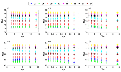
For the sake of finding the variation trend of the auroral oval boundary with the change in solar wind parameters, including solar wind density (N_p), solar wind speed (V_p), and solar wind dynamic pressure (P_dyn) respectively, experiment 2 is performed. Figure 6 shows the response of different solar wind parameters on the auroral oval boundary.

From Fig. 6, both the poleward and equatorward boundaries shrink at 21:00–06:00 MLT when the value of N_p rises. Meanwhile, the poleward and equatorward boundaries at 09:00–18:00 MLT gradually approach the Equator when the value of N_p rises. In addition, we can draw the following conclusions: the poleward and equatorward boundaries at 03:00–18:00 MLT extend to the Equator clearly with the increase in P_dyn, and the equatorward boundary at 21:00–24:00 MLT has a poleward motion with the increase in P_dyn. There is an obvious poleward motion in the nightside sector impacted by the increasing P_dyn and N_p according to the conclusions above. We can make a coincident inference with previous studies, for example, poleward displacement of the auroral oval boundary along with the increasing P_dyn, which results from the shrunken polar cap (Cho et al., 2010). B_y extension, there must have been some dependencies between the varying size of the polar cap and nightside reconnection (Boudouridis et al., 2003). Compared with the change in the auroral oval boundary in the nightside sector, both the poleward and equatorward boundaries are enlarged when the values of P_dyn and N_p rise, which is observed from Fig. 6. Previous explorations and simulations have shown that enlarged P_dyn can enhance ionospheric potential and the corresponding field-direction current intensity, which can lead to an increase in global auroral activity intensity. Meanwhile, the position of the auroral oval boundary will extend to low latitudes (Peng et al., 2011). From Fig. 6, a distinct equatorward movement appears with an increase in V_p at 24:00–06:00 MLT for both the poleward boundary and the equatorward boundary. This changing pattern of V_p and the auroral oval boundary which we illustrate above is consistent with Hu's study in 2017 (Hu et al., 2017).

Figure 7 Response of the magnetic latitude of poleward (a, b, c) and equatorward (b, e, f) boundaries to AE, AU, and AL respectively at 00:30, 00:60, 00:90, 12:00, 15:00, 18:00, 21:00, and 24:00 MLT.

3.3.3 Experiment 3. Influence of geomagnetic indexes on the auroral oval boundary

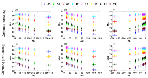
In this experiment, the average tendency of the poleward and equatorward boundaries influenced by geomagnetic indexes (AE, AL, AU) is shown in Fig. 7.

As we can see from Fig. 7, in every MLT sector, the poleward and equatorward boundaries move to low magnetic latitude with the ascending AE and AU indexes, while the poleward and equatorward boundaries extend to high magnetic latitude with the ascent of the AL index. The AE index is often used to characterize the strength of substorm activity in the magnetosphere. Therefore, it can be considered that the auroral oval extends to the Equator due to the enhanced substorm activity. Furthermore, the amount of energy enters the magnetotail along with the strengthening of substorm activity. This means that the AE index will increase when energy in the magnetotail is released through a substorm, which is coincident with our findings about AE from Fig. 7.

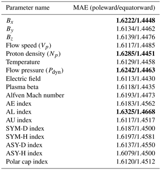
Table 3 The MAE influenced by different space physical parameters. The bigger MAE values in both the poleward and equatorward boundaries were written in bold font compared with others. The values written in bold font representing its corresponding space physical parameters had more influence on poleward and equatorward boundaries.

3.3.4 Experiment 4. Influence of all 18 space physical parameters on the auroral oval boundary

As we know, most of the studies on how the space physical parameters affect the auroral oval boundary focus on solar wind parameters, geomagnetic indexes, and IMF components. There have been lots of corresponding conclusions about the influence of those space physical parameters on the auroral oval boundary up to now. Nonetheless, how the other space physical parameters not mentioned above affect the auroral oval location has not been addressed. In order to further explore the variation of the auroral oval boundary influenced by different space physical parameters, experiment 4 is performed. In experiment 4, we send one physical parameter selected from Table 1 at the present moment and the coordinates of auroral oval boundary points at the previous moment to our prediction model, and the outputs of our model are 48 coordinate values of auroral oval boundary points and the MAE between real boundaries and predicted boundaries. The MAE values of poleward and equatorward boundaries influenced by different space physical parameters are given in Table 3. We can infer the response of the auroral oval boundary to 18 space physical parameters through the different MAE values of these space physical parameters.

The MAE values of the boundary positions are 1.6076 and 1.4545 respectively when we only use boundary positions at the previous moment to predict poleward and equatorward boundaries. We take this MAE as standard, called S-MAE. Compared with the S-MAE, we can see that the MAE increases about 1.9 % for the poleward boundary by adding any one space physical parameter to the input of our model from Table 3. Meanwhile, the value of MAE for the equatorward boundary is between −0.7 % and 0.7 %. Although different space physical parameters have different influences on the auroral oval boundary, compared to other space physical parameters in Table 3, the MAE of the auroral oval boundary can display the greatest impact when AL, B_x, N_p, and P_dyn are used as the inputs of our model respectively, which suggests that these four space physical parameters mentioned above have a great influence on the position of the auroral oval boundary.

Table 4 The Pearson correlation coefficient of all 18 space physical parameters from December 1996 to March 1997.

3.3.5 Experiment 5. Correlation analysis of all 18 space physical parameters

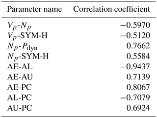
In order to analyse the influence of space physical parameters on the auroral oval efficiently, we not only consider the effect of each space physical parameter on the auroral oval boundary, but also take the effect on the auroral oval boundary with different combinations of space physical parameters into account in experiment 5. As a result, we first calculate the correlations of all 18 space physical parameters using the Pearson correlation coefficient, which is a statistical value that reflects the degree of linear correlation between two variables. The Pearson correlation coefficient of two variables (XY) equals the covariance of the two variables (XY) divided by the product of their standard deviations (σ_Xσ_Y). The formula of the Pearson correlation coefficient can be represented as Eq. (6), and the Pearson correlation coefficients of all 18 space physical parameters are given in Table 4. The process of experiment 5 is similar to experiment 4 and the MAE values of different space physical parameter combinations are given in Table 5.

$$\begin{array}{}\text{(6)}& {\mathit{\rho }}_{X,Y}={\displaystyle \frac{\mathrm{cov}(X,Y)}{{\mathit{\sigma }}_X{\mathit{\sigma }}_Y}}={\displaystyle \frac{E\left[\left(X-{\mathit{\mu }}_X\right)\left(Y-{\mathit{\mu }}_Y\right)\right]}{{\mathit{\sigma }}_X{\mathit{\sigma }}_Y}}\end{array}$$

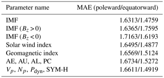
The MAE values of the poleward and equatorward boundaries by using three components of IMF and auroral oval boundary positions which were acquired at the last moment as the input of the proposed model are 1.6313 and 1.4759 respectively in Table 5. The MAE values of the three components of the IMF combination are bigger than S-MAE. When the input of our model includes B_x, B_y, and B_z, it is obvious that the MAE values of the poleward and equatorward boundaries both have significant increases compared with the MAE values of the poleward and equatorward boundaries by inputting any IMF components into our model, which suggests that the three components of the IMF have a similar influence on the auroral oval boundary. Previous investigations illustrated that the auroral oval boundary is connected with the variation of IMF B_x, B_y, and B_z (Huang et al., 2000; Provan et al., 1999). Our experiment results also demonstrate that the auroral oval boundary should be related to the three components of the IMF. When the northward or southward IMF directions are inputted into the proposed model, the MAE values have marked changes in both the poleward and equatorward boundaries. Nevertheless, we can observe the more evident increase in MAE in the equatorward boundaries compared with the MAE of the poleward boundaries by using the northward IMF direction as the input of our model. Meanwhile, there was an opposite result under the southward IMF direction condition. The variations of MAE in the poleward boundaries are bigger than those of the equatorward boundaries when the input of our model is in the southward IMF direction. Therefore, we can know that the northward IMF direction has a great influence on the equatorward boundaries, and the southward IMF direction has a significant effect on the poleward boundaries.

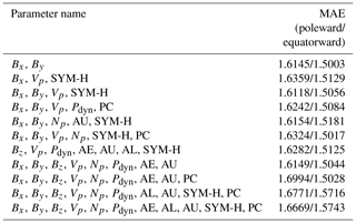
We can see that AE has a strong positive correlation with AU and PC and that AL has a strong negative correlation with AE, AU, and PC from Table 4. The linear correlation coefficient between AE and AL is −0.9437, which verified that the AL index has the opposite effect on the auroral boundary compared with the AE index. In contrast, the impact of the AU index on the auroral boundary is similar to the impact of the AE index on the auroral boundary because of the strong positive correlation between AE and AU. Those conclusions mentioned above are consistent with the conclusions of statistical experiment 3. In addition, the correlation coefficient between AE and PC is 0.8067, which implies PC should have a homologous trend with AE in every MLT section. Figure 8 shows the response of the poleward and equatorward boundaries to PC respectively. The PC index can serve as an indicator of auroral electrojet activity. Vennerstrøm found that PC is sensitive to electrojet activity and substorm intensifications of the westward electrojet in the midnight or post-midnight sectors (Vennerstrøm et al., 1991). This conclusion matches what we found about the impact of PC on the auroral oval boundary in Fig. 8. When the input of our model only included the three geomagnetic indices (AE, AL, AU) and the auroral oval boundary positions at the previous moment, the MAE values of the equatorward and poleward boundaries are 1.6569 and 1.5124 respectively from Table 5. We can clearly know that the MAE values of the poleward and equatorward boundaries are both enlarged compared with S-MAE. As a result, we can draw the conclusion that the three geomagnetic indexes strengthen each other's effect when the combination of the three geomagnetic indexes is inputted into our model. Beyond that, in Table 5, when AE, AU, AL, and PC are used as the input of our model, the MAE values of poleward and equatorward boundaries are 1.6734 and 1.5275 respectively, which shows that the combinations of those parameters have an important influence on the location of the auroral oval boundary.

Table 5 The MAE influenced by different combinations of space physical parameters.

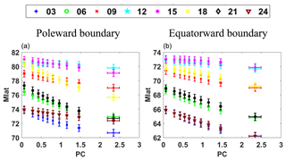
Figure 8 Response of the magnetic latitude of poleward (a) and equatorward (b) boundaries to PC at 00:30, 00:60, 00:90, 12:00, 15:00, 18:00, 21:00, and 24:00 MLT.

Table 6 The MAE influenced by different combinations of space physical parameters.

According to Table 4, there was an obvious correlation among the following space physical parameters. For the solar wind parameters, V_p and N_p are positive correlations, while N_p and P_dyn are negative correlations, and the three parameters are all related to SYM-H. Firstly, we can obtain a similar inference on the three geomagnetic indices to solar wind parameters (V_p, N_p, P_dyn) according to the MAE values of the three solar wind parameter combinations from Table 5 and the strong correlation between them. In other words, the three solar wind parameters also strengthen each other's effect on the auroral oval boundary when the combinations of them are sent into our model. Secondly, when N_p, V_p, P_dyn, and SYM-H are input into our model, the MAE values of the auroral oval boundaries are 1.6611 and 1.4919 poleward and equatorward respectively in Table 5, which is bigger than the MAE values of the auroral oval boundaries when the inputs are N_p, V_p, and P_dyn. So, we can conclude that the combinations of these four parameters strengthen the mutual influence on the location of the auroral oval boundary. According to the statistics from Table 6, the physical variables that appear most frequently are B_x, B_y, V_p, and SYM-H. When the inputs of our model are the combination of these four variables or the combination of B_x and B_y, the MAE of the auroral oval boundary reaches its minimum, which proves that these four parameters have a great influence on the location of the auroral oval boundary.

As a summary, it can be seen that these space physical parameters, which include B_x, B_y, V_p, and SYM-H, play a crucial role in determining the location of the auroral oval boundary based on the above conclusions.

4 Conclusions

In this paper, we establish a model to measure the relationship between space physical parameters from the OMNI dataset on the NASA website and poleward and equatorward auroral oval boundaries based on a deep learning network. Our model overcomes some drawbacks in this field, such as some prediction methods based on statistics and a few space physical parameters. Those methods are not very suitable for the complex and changeable space physical data. For our model, the inputs are 18 space physical parameters and the 48 coordinates value of auroral oval boundary points at the previous moment, and we can obtain positions of poleward and equatorward boundaries at 24 MLTs from our well-trained model. At last, our experiment results show that the model proposed in this paper can better reflect the relationship between space physical parameters and an auroral oval boundary. Therefore, it should be useful to predict the position of an auroral oval boundary. In addition, we analyse the effect of all 18 space physical parameters on the location of an auroral oval boundary based on several statistical and prediction experiments. It can be shown that different parameters have different effects on the auroral oval boundary from our experiments. Some space physical parameters, B_x, B_y, V_p, and SYM-H, have a great influence on the position of the auroral oval boundary.