the Creative Commons Attribution 4.0 License.
the Creative Commons Attribution 4.0 License.
 | 30 Jan 2020
Magnitude correlations in a self-similar aftershock rates model of seismicity
Andres F. Zambrano Moreno
Jörn Davidsen
Crucial to the development of earthquake forecasting schemes is the manifestation of spatiotemporal correlations between earthquakes as highlighted, for example, by the notion of aftershocks. Here, we present an analysis of the statistical relation between subsequent magnitudes of a recently proposed self-similar aftershock rates model of seismicity, whose main distinguishing feature is that of interdependence between trigger and triggered events in terms of a time-varying frequency–magnitude distribution. By means of a particular statistical measure, we study the level of magnitude correlations under specific types of time conditioning, explain their provenance within the model framework and show that the type of null model chosen in the analysis plays a pivotal role in the type and strength of observed correlations. Specifically, we show that while the variations in the magnitude distribution can give rise to large trivial correlations between subsequent magnitudes, the non-trivial magnitude correlations are rather minimal. Simulations mimicking southern California (SC) show that these non-trivial correlations cannot be observed at the 3σ level using real-world catalogs for the magnitude of completeness as a reference. We conclude that only the time variations in the frequency–magnitude distribution might lead to significant improvements in earthquake forecasting.
- Article
(3523 KB) - Full-text XML
-
Supplement
(676 KB) - BibTeX
- EndNote


An outstanding question in earthquake dynamics is how reliably one is able to predict or forecast earthquakes. Forecasting can be defined as a statement of the relative likelihood of specific earthquake(s) occurring as a function of space, time and magnitude windows, and it should be contrasted with the concept of prediction, which is a specific statement as to whether an earthquake will or will not occur at a particular place and time with a certain magnitude (Jackson and Kagan, 1999). In recent years, the forecasting of earthquakes has seen a major effort on many different fronts (Gerstenberger et al., 2005; Helmstetter et al., 2006; Holliday et al., 2007; Schorlemmer et al., 2010; Woessner et al., 2010; Zechar et al., 2010; Field and Milner, 2018; Moschetti et al., 2018; DeVries et al., 2018); also see Ogata (2013), Ogata (2017), Tiampo and Shcherbakov (2013), and Michael and Werner (2018) for reviews. A defining characteristic of earthquakes is their clustering in both space and time. By considering various empirical relations one can construct models (the backbone of a multitude of forecasting efforts), most being a special case of the Hawkes process (Hawkes, 1971). These include the epidemic-type aftershock sequence (ETAS) model (Ogata, 1988, 1998), the branching aftershock sequence (BASS) model (Turcotte et al., 2007), the every earthquake is a precursor according to scale (EEPAS) model (Evison and Rhoades, 2004; Rhoades and Evison, 2004) and a branching model based on a dynamical scaling hypothesis where a single dynamical scaling exponent was introduced in the conditional rate parameter (Lippiello et al., 2007a, b); all of these exhibit spatiotemporal clustering.
It is through the aforementioned constitutive statistical models that forecasting of seismicity is often implemented (Helmstetter et al., 2006; Schorlemmer et al., 2010; Woessner et al., 2010; Zechar et al., 2010). Temporal clustering is exemplified by the increased rate (number of earthquakes per unit time) of local seismicity after large earthquakes, where the triggering of earthquakes by other earthquakes through either static or dynamic stress changes is one of the predominant physical processes occurring over a wide range of spatiotemporal scales (Moradpour et al., 2014; Hainzl et al., 2014). The empirically derived Omori–Utsu relation (Omori, 1894; Utsu, 1957) is used to encode temporal clustering in many of the aforementioned models of seismicity; e.g., the extensively studied ETAS model employs this relation. Yet, in its original formulation the Omori–Utsu relation is typically not self-similar. By formulating the rate of earthquakes as a self-similar process which gives rise to a generalized Omori–Utsu relation, one finds greater agreement with observed seismic behavior in southern California (SC) when compared to the standard non-self-similar form (Davidsen and Baiesi, 2016). Such self-similarity provides support for the hypothesis that one can scale up constitutive rules derived from fracture and friction experiments in the lab to tectonic earthquakes (Scholz, 1990; Mogi, 2007). The self-similar aftershock rates (SSAR) model proposed in Davidsen and Baiesi (2016) is a model of earthquake–earthquake triggering, similar to the ETAS model. The SSAR model contains two distinguishing features; event rates are self-similar with respect to the magnitude difference between the trigger and the triggered event, and the frequency–magnitude distribution of the triggered events for a single trigger varies in time. In the standard Omori–Utsu relation the number of triggered events of a particular energy does not simply depend on the magnitude difference between trigger and triggered events (i.e., mother–daughter events). This relation is not self-similar unless very special conditions are met; conditions which are typically inconsistent with observations (Davidsen and Baiesi, 2016). The ansatz for a self-similar mother–daughter rate relation can be expressed as
where τΔm and cΔm are two timescales that only depend on , m′ and mas are the magnitudes of the trigger and triggered event, respectively, and t is the time interval between the trigger and triggered event. In Lippiello et al. (2007a, b) only one such dynamical scaling exponent was introduced in the conditional rate equation, and in Shcherbakov et al. (2015) the two timescales were first introduced along with the relation between the exponents of τΔm and cΔm, terms which we will present in detail in Sect. 2. Dependence on the magnitude difference for the two timescales allows one to obtain two scale-free regimes when considering the frequency–magnitude distribution of events triggered by events of the same magnitude: a feature consistent with observed behavior in the SC catalog (Davidsen and Baiesi, 2016) and shown to exist in the detailed analysis of aftershock rates in Japan (Peng et al., 2007). Furthermore, scaling of the form in Eq. (1) for a particular was shown to be consistent with all accepted empirical relations (Davidsen and Baiesi, 2016). Just as the ETAS model is widely used in forecasting efforts, one would wish to use the SSAR model for this particular purpose given that the latter was shown to better describe the SC seismic data. The main difference between the ETAS and SSAR models is that in the latter case the mother–daughter magnitudes are effectively coupled in accordance with Eq. (1). From this vantage point, one would like to quantify the strength of the statistical correlation of magnitudes in a time-ordered catalog in the SSAR model, which may ultimately aid in developing more reliable forecasting methods. For this purpose, the magnitude correlations between subsequent events are of particular interest. In order to study magnitude correlations between subsequent events, we apply here a statistical method similar to the ones employed in Lippiello et al. (2008), Davidsen and Green (2011), and Davidsen et al. (2012). An important aspect to highlight is that in our analysis we test two different types of null hypotheses against the SSAR model. We find that the null hypothesis plays a significant role in the types and strength of magnitude correlations observed. This allows us to distinguish between trivial magnitude correlations that are simply a consequence of the variations in the frequency–magnitude distribution and non-trivial ones that are not.
Overview of this paper
We first give a brief overview of the SSAR model (Sect. 2), introduce the specifics of the surrogate catalogs (Sect. 2.1), follow that with the methodology (Sect. 3.1) and analysis of the magnitude correlations between subsequent events through the lens of a particular statistical measure (Sect. 3.2, 3.3). In the latter, we show why it is important that in the analysis of magnitude correlations care must be taken with the methodology (on choosing the randomized magnitudes, i.e., the type of null model) if one wishes to avoid confounding factors. In Sect. 4 we present a discussion of our results.
The SSAR model recasts the standard Omori–Utsu rate equation into a self-similar version. A distinguishing feature of the rate equation in the SSAR model is that it only depends on the difference between mother–daughter events making it self-similar (e.g., the rates of a magnitude 3 mother and magnitude 2 daughter event are the same as those of a magnitude 5 mother and a magnitude 4 daughter event); the scaling relation along with the relationship amongst its exponents was explored in the context of the rates for all events above a magnitude m along with the use of Båths relation in Shcherbakov et al. (2015) and formulated in Davidsen and Baiesi (2016) in the form we will use in this paper as
with timescales,
where g and z are universal scaling exponents – with corresponding simulation values of 0.66 and 0.24 matching SC (Davidsen and Baiesi, 2016) – c0 and τ0 are constant prefactors (with respective values of 210 and 104 s in the simulations), and p≳1 (Davidsen and Baiesi, 2016) (p≤1 is unphysical if considering only daughter events, i.e., directly triggered events; see, for example, Davidsen et al., 2015). To obtain the total number of triggered events of magnitude mas for a given trigger m′, we integrate Eq. (2) in the time domain
which only depends on Δm ensuring self-similarity. Integrating Eq. (4) from a chosen cutoff magnitude mcut to ∞, we find
which is simply the Gutenberg–Richter relation for triggered events (Davidsen and Baiesi, 2016), giving us the scaling relation (Shcherbakov et al., 2004),
In contrast, for finite times the number of triggered events of magnitude mas up to a time tf is
Plotting Eq. (7) for different values of tf in Fig. 1, we observe a defining characteristic of the SSAR model. Unlike another self-similar model (Lippiello et al., 2007a, 2008), two scale-free regimes coexist for all finite values of tf in the frequency–magnitude distribution, an effect recognized during different stages of aftershock sequences in Shcherbakov et al. (2004). Namely, b→z corresponds to the dominating exponent in the early time limit of Eq. (2), and a second regime with dominates at later times. In other words, at early times we can observe a b value of z over an extended regime of small magnitudes, but as tf increases, the transition point moves towards smaller magnitudes, and we begin to see a more extended range with a b value of g+z, which corresponds to the asymptotic behavior for tf→∞.
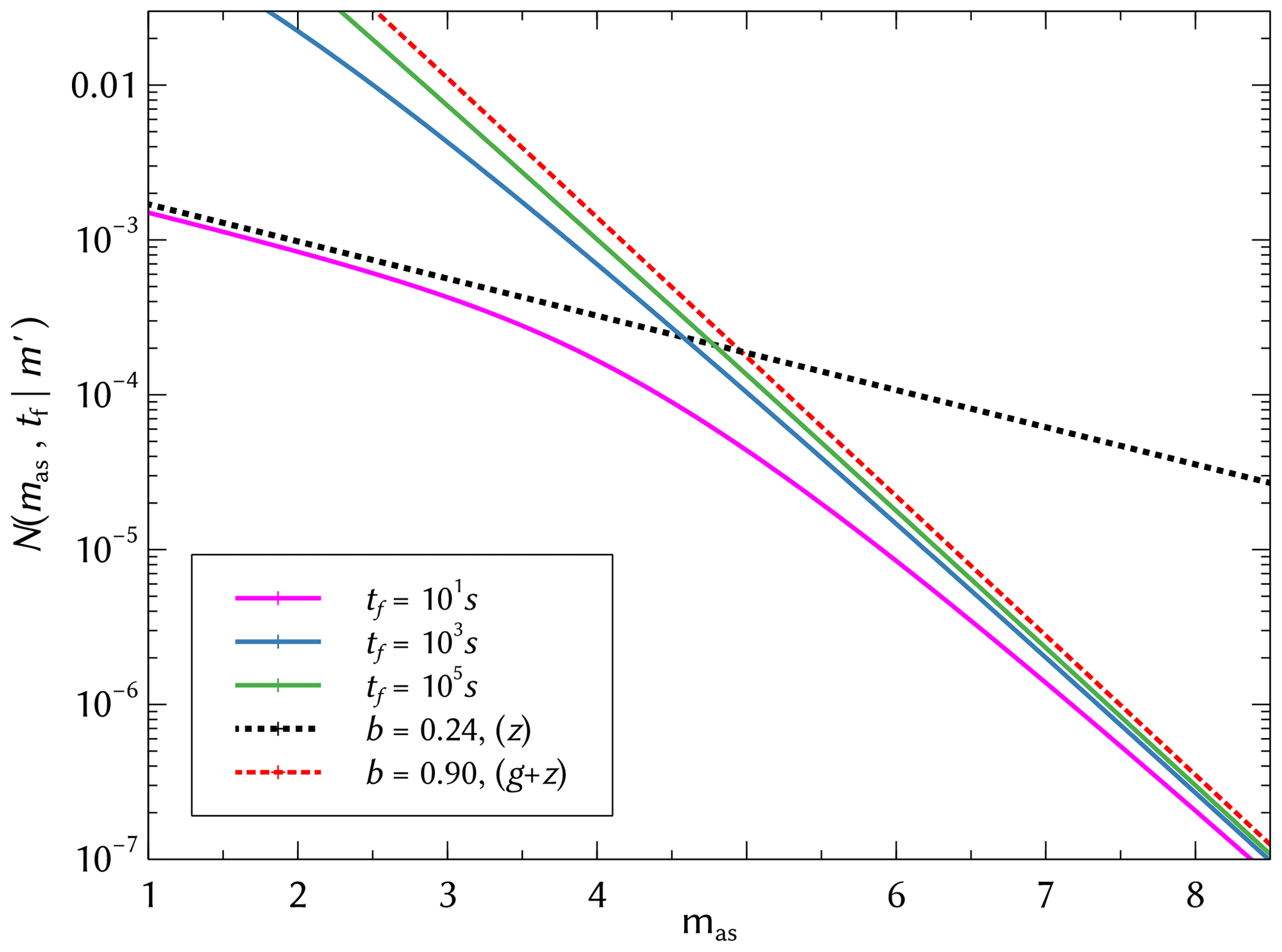
Figure 1Plot of Eq. (7) for and tf=101, 103 and 105 s. Dashed lines correspond to the b value exponent; b=z for early times (black), and for late times (red).
Analogously to the ETAS model, the full SSAR model is given by a time-varying seismic rate (also called the conditional intensity or stochastic intensity), which takes on the following form:
where μ is a constant and s0(m) is the probability density function (PDF) of the magnitudes of background events, i.e., events that are not triggered by other events. The product of these determines the background rate, which is assumed to be uniform in time and space. Similarly, and are the PDFs for the temporal distance, magnitude and spatial distance of daughter events triggered by a mother of magnitude m′, respectively. κ(m′) corresponds to the total number of daughters triggered by a mother, often denoted as the productivity relation. For the purpose of our temporal analysis of magnitudes, we can ignore the spatial component in Eq. (8), and we refer the reader to Moradpour et al. (2014) and Davidsen and Baiesi (2016) for a treatment of . The PDFs for the magnitude distribution of background and triggered events are the normalized Gutenberg–Richter relations.
where mcut indicates the lower magnitude cut-off, β=bln 10 – with simulation value b=1.08 matching SC (Davidsen and Baiesi, 2016) – and βas=basln 10. The productivity relation and the normalized temporal distribution for the generalized Omori–Utsu relation are, respectively,
SSAR model catalogs
Since the SSAR model was tested using a catalog from SC (Davidsen and Baiesi, 2016), we focus here on synthetic model catalogs that are comparable to those from SC. We would like to point out again that for the purpose of our analysis of magnitude correlations below, the spatial location of events is not relevant. A seismic catalog generated through the SSAR model consists of both independent background events and its associated nth generation aftershocks. The catalog is generated by first seeding background events with magnitudes selected from the corresponding frequency–magnitude distribution of Poissonian times; triggered events are then created from the statistical distributions of magnitude and time in an iterative manner (see Sect. S2 in Supplement of Davidsen and Baiesi, 2016, for details). A realization of the SSAR model, which resembles the SC catalog, henceforth referred to as SSAR-SC, was used for the analysis presented in this paper, see Fig. 2. Yet, none of our findings depend on the specific realization, as we tested explicitly. The SSAR-SC catalog contains background events with a total of 376 311 events (after removing 1 % of the initial events to minimize boundary effects), a lower magnitude cutoff of mmin=1.50, and model parameters of p=1.15, c0=210 s, τ0=104 s, g=0.66 and z=0.24 that agree with those of SC (Davidsen and Baiesi, 2016). This corresponds to a coverage of about 36 years, the current length of the relocated SC catalog from 1981 to 2017 (Hauksson et al., 2012). We have also imposed a hard upper cutoff, Mmax=7.40, for the largest magnitude possible in the SSAR-SC catalog in order to avoid an unphysical runway process.

Figure 2Time–magnitude plot for a realization of the SSAR model with a lower magnitude threshold of 1.50 and 376 311 events.
In this section we aim to answer the question of what is the type and strength of the effective magnitude correlations in the SSAR model (for an analysis of magnitude correlations in the SC catalog, see Davidsen and Green, 2011). Correlations arise by means of the rate equation given by Eq. (2) since the timing of the daughters will depend on the magnitude difference between the daughters and mothers as captured by the functional dependencies of cΔm and τΔm. We first draw attention to the methodology since this is a crucial aspect in understanding the types of correlations observed in the model.
3.1 Methodology
Our study of magnitude correlations, similar to methods used in Lippiello et al. (2008), Davidsen and Green (2011), and Davidsen et al. (2012), considers subsequent events in the time ordered catalog. Specifically, it focuses on (for particular magnitude thresholds mth) and compares these to randomized magnitude differences averaged over 500 realizations, i.e., , where is a magnitude chosen at random. If magnitude correlations between subsequent events in the ordered catalog are present, the distribution of Δm will deviate from the distribution of the randomized case, Δm*. To assess whether magnitude correlations exist in the SSAR model we considered three types of conditioning (unconditioned, Δt and Δt & M–D (mother–daughter)) for various magnitude thresholds mth. For the unconditioned case we use the quantity , where P(…) refers to the cumulative distribution function (CDF) of the ordered and randomized catalogs. For Δt and Δt & M–D conditioning, we consider the corresponding quantities:
and
Specifically, for Δt and Δt & M–D conditioning one only considers subsequent event pairs and their Δmi if the time interval between the two events is not longer than Δt. In addition, for Δt & M–D conditioning these event pairs also have to be a mother–daughter pair. The reason why we choose to condition on time intervals is motivated by the expectation that event pairs that are closer in time are more likely to be related – either by being mother–daughter pairs or by being daughters of the same mother – than those further apart. Note that in the SSAR model all dependencies are fundamentally encoded at the mother–daughter level, viz. Eq. (2). By conditioning on time we are also preferentially picking certain magnitude differences via the rate equation, Eq. (2).
Another important aspect in our analysis is how we randomly choose the magnitudes in the case of Δt or Δt & M–D conditioning. One can either pick values from the already conditioned catalog – which we call sub-catalog randomizing – or pick values from the full unconditioned catalog – called full-catalog randomizing. It is important to point out that in sub-catalog randomizing the frequency–magnitude distributions of mi+1 and are identical by construction. In full-catalog randomizing, however, the might or might not follow a different frequency–magnitude distribution. This is possible since the frequency–magnitude distribution can vary in the SSAR model as discussed above. A similar and more graphical explanation of sub- and full-catalog randomizing can be found in the Supplement.
For all three types of conditioning one can state the following. If the quantity δP(m0|…) significantly deviates from 0 for at least some values of m0, then correlations between subsequent magnitudes are present. The two randomizing methods used in our analysis (one keeps the frequency–magnitude distribution fixed, while the other one might not) both produce in principle different types of magnitude correlations. When the frequency–magnitude distribution is fixed, we are seeing inherent (non-trivial) magnitude correlations, while the correlations in the other case correspond to a mixing of non-trivial and trivial correlations, where the latter simply arise due to the differences in the frequency–magnitude distribution.
3.2 Magnitude correlations for the unconditioned case of the SSAR model
In Fig. 3 we show the previously described measure of magnitude correlations for subsequent events for the unconditioned case in the SSAR-SC catalog. Magnitude correlations that are significant at the 3σ level exist in the SSAR-SC catalog in the range mth=1.60–2.80. Inspecting the slope of δP(m0) in Fig. 3, we see that the values Δm have a higher tendency to lie in a given range when compared to the randomized case Δm* and are less likely to lie outside said range: for mth<2.4 the slope of δP is typically positive in the range −0.5 to 0.25 showing an ≈0.9 % higher probability that Δm lies within this range when compared to Δm*. While significant, this difference is very small. The absence of significant correlation at the 3σ level for mth=3.40 (the current magnitude of completeness for SC; Schorlemmer and Woessner, 2008) is simply a consequence of an insufficient number of events.
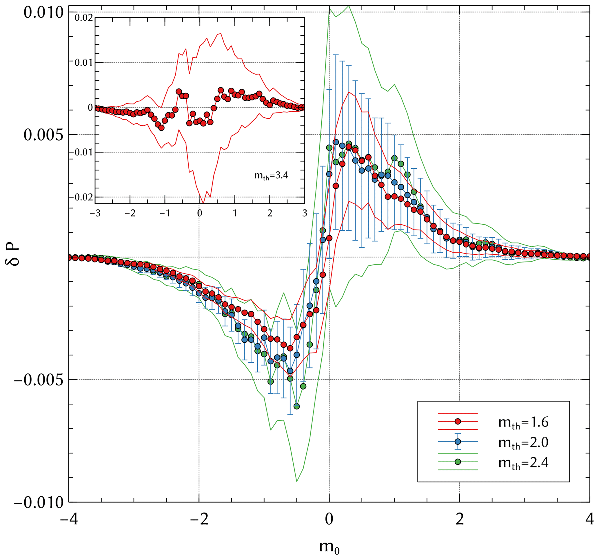
Figure 3Magnitude correlations of the unconditioned SSAR-SC catalog for mth=1.60, 2.00, 2.40 and 3.40 (inset). Error bars correspond to 3σ.
3.3 Δt & M–D conditioning in the SSAR model
To test whether magnitude correlation becomes stronger if one considers pairs of events that are related, we now focus on the magnitude correlation analysis for Δt & M–D conditioning. The correlations that arise under Δt & M–D conditioning are shown in Fig. 4. The two randomization types produce vastly different results. For sub-catalog randomizing (Fig. 4a), we see no qualitative difference in the shape of compared to the unconditional case. Yet, the probability of encountering a magnitude difference in an interval around 0, i.e, a daughter event being similar in magnitude to the mother event, is now up to 4 times higher for the smallest Δt than for δP(m0) (Fig. 3). Even for there is a significant increase in the excess of daughters that are on average the same size as the mother to about 2.6 %. As before, this excess comes at the expense of significantly smaller and larger daughter events. As Fig. 4c shows, a similar behavior occurs for larger mth values.
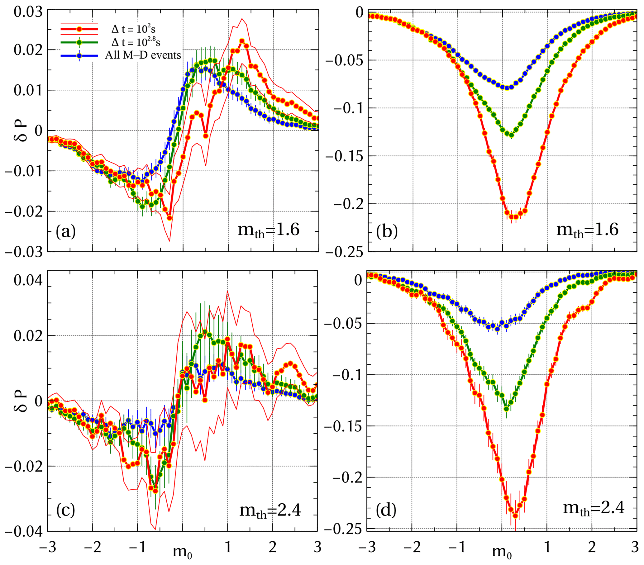
Figure 4Magnitude correlations for the SSAR-SC catalog with Δt & M–D conditioning for sub-catalog randomizing (a, c) and full-catalog randomizing (b, d) for mth=1.60 and 2.40. To see the trends clearly, only 1σ error bars are shown.
In contrast, when estimating using full-catalog randomizing (Fig. 4b), the distribution is qualitatively and quantitatively distinct compared to δP(m0). Specifically, Fig. 4b demonstrates that independent of the Δt values, the magnitudes of the daughter events tend to be on average larger than those of the mother events compared to what is expected based on the null model. The associated probability increases from a minimum of 8 % to over 20 % for increasing values of Δt. As Fig. 4d shows, a similar behavior occurs for larger mth values.
As discussed above, the underlying difference between sub-catalog and full-catalog randomizing for Δt & M–D conditioning is the frequency–magnitude distribution of the randomized daughter events (cf., end of Sect. 3.1). Thus, our observations indicate that the non-trivial magnitude correlations captured by sub-catalog randomizing are significant but smaller by up to a factor of 6 for Δ=102 s and mth=2.4 compared to the mixture of trivial and non-trivial magnitude correlations measured by using full-catalog randomizing. This indicates that the trivial magnitude correlations arising from differences in the frequency–magnitude distribution significantly outweigh the non-trivial ones under appropriate conditioning and play the more dominant role.
While in our model simulations we can readily identify mother–daughter pairs, i.e., the ground truth is known, this is not the case for field data. Thus, for such catalogs – including the SC catalog – one would need to infer mother–daughter pairs, i.e., decluster the catalog first (Baiesi and Paczuski, 2004; Zaliapin et al., 2008; Marsan and Lengliné, 2008; Zaliapin and Ben-Zion, 2013; Gu et al., 2013), in order to estimate the magnitude correlations for Δt & M–D conditioning. As an alternative, time conditioning alone has been used in the past (Lippiello et al., 2008; Davidsen and Green, 2011; Davidsen et al., 2012). This is what is shown in Fig. 5. When compared to Fig. 4, a significant decrease in amplitude of δP can be observed. This decrease is especially large for small mth values. Yet, as before, the trivial magnitude correlations arising from differences in the frequency–magnitude distribution significantly outweigh the non-trivial ones.
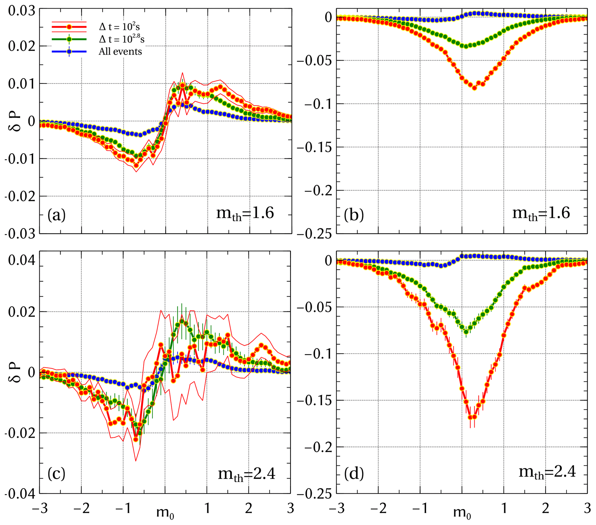
Figure 5Magnitude correlations for the SSAR-SC catalog with Δt conditioning for sub-catalog randomizing (a, c) and full-catalog randomizing (b, d) for mth=1.60 and 2.40. To see the trends clearly, only 1σ error bars are shown.
To clarify the reason for the difference between the Δt & M–D conditioning and the Δt conditioning, we can examine the ratio of event pairs within Δt that show mother–daughter relations to all event pairs that fall within the time interval Δt in the SSAR model (Fig. 6). According to Fig. 6, in order to maximize the ratio of mother–daughter events one should choose subsequent event pairs that have a high mth and are close in time (small Δt). This explains the differences between two different types of conditioning shown in Fig. 4 and in Fig. 5, which become less pronounced for higher mth and smaller Δt values.
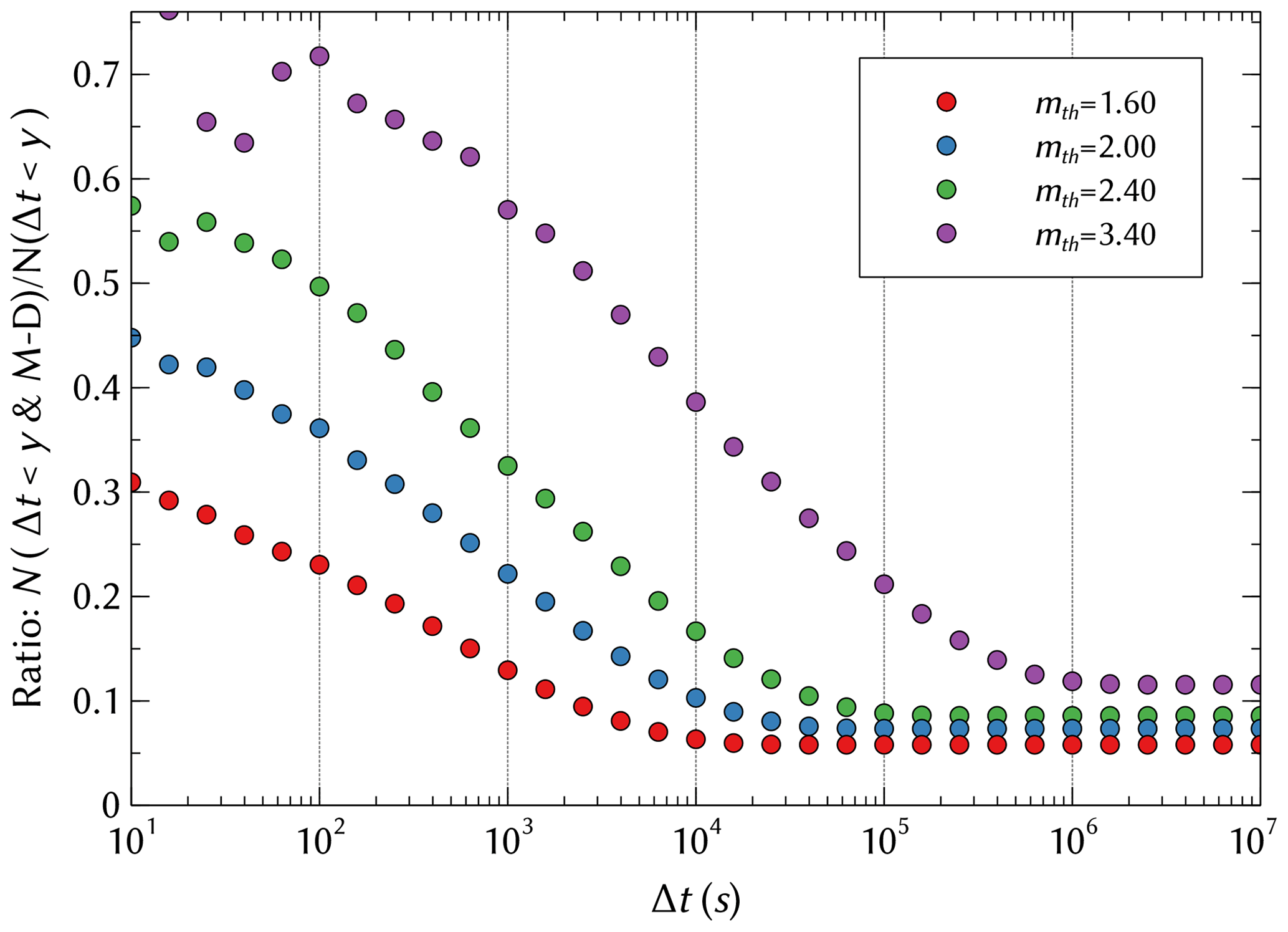
Figure 6Ratio of total number of events satisfying Δt<y & M–D to Δt<y conditioning for the SSAR-SC catalog for different values of mth.
The aforementioned maximization comes with a trade-off; although a higher mth value captures more mother–daughter pairs, the total number of selected event pairs goes down at the same time leading to higher statistical uncertainties. It is also important to realize that the ratios shown in Fig. 6 are for the specific parameters used in our realization of the SSAR model (cf. Sect. 2.1). Choosing different parameter values for c0 and τ0, for example, will effect the specific ratio even if one keeps c0∕τ0 constant, though the qualitatively behavior remains the same.
Through a particular statistical measure (Sect. 3.1) we have shown how two different types of magnitude correlations between subsequent events arise in the SSAR model (Sect. 3.3). Trivial correlations are largely a consequence of variations in the frequency–magnitude distribution, while this is not the case for non-trivial correlations, similar to what has been discussed in the context of tectonic seismicity (Davidsen and Green, 2011). Both types of correlations can be estimated by using different underlying null models, implemented here by the two different types of catalog randomizing. Given that magnitudes in the SSAR model are not independent (as exemplified in Eq. 2), it does not come as a surprise that non-zero magnitude correlations exist. We were able to explicitly show that it is indeed the mother–daughter pairs that are largely responsible for these correlations. Based on this, we were also able to show that one can increase the observed magnitude correlations by conditioning on shorter time intervals and considering higher values of mth (cf. Fig. 6). This is an important fact one can use when triggering relations are unknown or unavailable or when only information on time intervals is available, such as in the case of real-world catalogs. When dealing with real-world catalogs one needs, however, to consider the effects due to the magnitude of completeness and short-term aftershock incompleteness as well (Kagan, 2004; Moradpour et al., 2014; Hainzl, 2016).
Finally, the significantly higher strength of the trivial correlations compared to the non-trivial correlations is the main outcome of our analysis. Thus, when it comes to improving earthquake forecasting efforts our analysis leads us to believe that looking at the time variations in the frequency–magnitude distribution could perhaps be a more fruitful approach then focusing on non-trivial correlations. Using the SSAR model instead of the ETAS model in existing forecasting frameworks would be one way to utilize this. This remains a challenge for the future.
Python code, synthetic catalog data and plot data can be found in Zambrano Moreno (2019) (https://doi.org/10.5683/SP2/PGYQEV). Code and data are under the GPLv3 license (https://www.gnu.org/licenses/gpl-3.0.en.html, GNU, 2018). Data for southern California were downloaded from http://scedc.caltech.edu/research-tools/alt-2011-dd-hauksson-yang-shearer.html (Hauksson et al., 2017). For the methodology used on the SC catalog, see Hauksson et al. (2012) (https://doi.org/10.1785/0120120010).
The supplement related to this article is available online at: https://doi.org/10.5194/npg-27-1-2020-supplement.
AFZM prepared the paper with corresponding discussions, edits, contributions and modifications from JD. AFZM developed the model code, statistical analysis code and created the figures.
The authors declare that they have no conflict of interest.
Andres F. Zambrano Moreno would like to thank Jordi Baro for providing ETAS C++ code which helped greatly in understanding the type of coding that would be required for the creation of the SSAR code and for helpful consultations, Mohammed Yaghoobi for helpful discussions on the interpretation of the magnitude correlation plots, and Ayush Mandawal for lending an ear and participating in general dialogues on the topic.
This research has been partially supported by NSERC through a Discovery Grant to Jörn Davidsen.
This paper was edited by Ilya Zaliapin and reviewed by Robert Shcherbakov and one anonymous referee.
Baiesi, M. and Paczuski, M.: Scale-Free Networks of Earthquakes and Aftershocks, Phys. Rev. E, 69, 066106, https://doi.org/10.1103/PhysRevE.69.066106, 2004. a
Davidsen, J. and Baiesi, M.: Self-Similar Aftershock Rates, Phys. Rev. E, 94, 022314, https://doi.org/10.1103/PhysRevE.94.022314, 2016. a, b, c, d, e, f, g, h, i, j, k, l, m, n
Davidsen, J. and Green, A.: Are Earthquake Magnitudes Clustered?, Phys. Rev. Lett., 106, 108502, https://doi.org/10.1103/PhysRevLett.106.108502, 2011. a, b, c, d, e
Davidsen, J., Kwiatek, G., and Dresen, G.: No Evidence of Magnitude Clustering in an Aftershock Sequence of Nano- and Picoseismicity, Phys. Rev. Lett., 108, 038501, https://doi.org/10.1103/PhysRevLett.108.038501, 2012. a, b, c
Davidsen, J., Gu, C., and Baiesi, M.: Generalized Omori-Utsu Law for Aftershock Sequences in Southern California, Geophys. J. Int., 201, 965–978, https://doi.org/10.1093/gji/ggv061, 2015. a
DeVries, P. M. R., Viégas, F., Wattenberg, M., and Meade, B. J.: Deep Learning of Aftershock Patterns Following Large Earthquakes, Nature, 560, 632–634, https://doi.org/10.1038/s41586-018-0438-y, 2018. a
Evison, F. F. and Rhoades, D. A.: Demarcation and Scaling of Long-Term Seismogenesis, Pure Appl. Geophys., 161, 21–45, https://doi.org/10.1007/s00024-003-2435-8, 2004. a
Field, E. H. and Milner, K. R.: Candidate Products for Operational Earthquake Forecasting Illustrated Using the HayWired Planning Scenario, Including One Very Quick (and Not-So-Dirty) Hazard-Map Option, Seismol. Res. Lett., 89, 1420–1434, https://doi.org/10.1785/0220170241, 2018. a
Gerstenberger, M. C., Wiemer, S., Jones, L. M., and Reasenberg, P. A.: Real-Time Forecasts of Tomorrow's Earthquakes in California, Nature, 435, 328–331, https://doi.org/10.1038/nature03622, 2005. a
GNU: GPLv3, available at: https://www.gnu.org/licenses/gpl-3.0.en.html (last access: 1 March 2019), 2018. a
Gu, C., Schumann, A. Y., Baiesi, M., and Davidsen, J.: Triggering Cascades and Statistical Properties of Aftershocks, J. Geophys. Res.-Sol. Ea., 118, 4278–4295, https://doi.org/10.1002/jgrb.50306, 2013. a
Hainzl, S.: Rate-Dependent Incompleteness of Earthquake Catalogs, Seismol. Res. Lett., 87, 337–344, https://doi.org/10.1785/0220150211, 2016. a
Hainzl, S., Moradpour, J., and Davidsen, J.: Static Stress Triggering Explains the Empirical Aftershock Distance Decay, Geophys. Res. Lett., 41, 8818–8824, https://doi.org/10.1002/2014GL061975, 2014. a
Hauksson, E., Yang, W., and Shearer, P. M.: Waveform Relocated Earthquake Catalog for Southern California (1981 to June 2011) Short Note, B. Seismol. Soc. Am., 102, 2239–2244, https://doi.org/10.1785/0120120010, 2012. a, b
Hauksson, E., Yang, W., and Shearer, P. M.: SCSN Catalog, available at: http://scedc.caltech.edu/research-tools/alt-2011-dd-hauksson-yang-shearer.html (last access: 19 October 2018), 2017. a
Hawkes, A. G.: Point Spectra of Some Mutually Exciting Point Processes, J. R. Stat. Soc. B, 33, 438–443, 1971. a
Helmstetter, A., Kagan, Y. Y., and Jackson, D. D.: Comparison of Short-Term and Time-Independent Earthquake Forecast Models for Southern California, B. Seismol. Soc. Am., 96, 90–106, https://doi.org/10.1785/0120050067, 2006. a, b
Holliday, J. R., Chen, C.-C., Tiampo, K. F., Rundle, J. B., Turcotte, D. L., and Donnellan, A.: A RELM Earthquake Forecast Based on Pattern Informatics, Seismol. Res. Lett., 78, 87–93, https://doi.org/10.1785/gssrl.78.1.87, 2007. a
Jackson, D. D. and Kagan, Y. Y.: Testable Earthquake Forecasts for 1999, Seismol. Res. Lett., 70, 393–403, https://doi.org/10.1785/gssrl.70.4.393, 1999. a
Kagan, Y. Y.: Short-Term Properties of Earthquake Catalogs and Models of Earthquake Source, B. Seismol. Soc. Am., 94, 1207–1228, https://doi.org/10.1785/012003098, 2004. a
Lippiello, E., Bottiglieri, M., Godano, C., and de Arcangelis, L.: Dynamical Scaling and Generalized Omori Law, Geophys. Res. Lett., 34, 23, https://doi.org/10.1029/2007GL030963, 2007a. a, b, c
Lippiello, E., Godano, C., and de Arcangelis, L.: Dynamical Scaling in Branching Models for Seismicity, Phys. Rev. Lett., 98, 098501, https://doi.org/10.1103/PhysRevLett.98.098501, 2007b. a, b
Lippiello, E., de Arcangelis, L., and Godano, C.: Influence of Time and Space Correlations on Earthquake Magnitude, Phys. Rev. Lett., 100, 038501, https://doi.org/10.1103/PhysRevLett.100.038501, 2008. a, b, c, d
Marsan, D. and Lengliné, O.: Extending Earthquakes' Reach Through Cascading, Science, 319, 1076–1079, https://doi.org/10.1126/science.1148783, 2008. a
Michael, A. J. and Werner, M. J.: Preface to the Focus Section on the Collaboratory for the Study of Earthquake Predictability 2CSEP169New Results(CSEPFuture Directions, Seismol. Res. Lett., 89, 1226–1228, https://doi.org/10.1785/0220180161, 2018. a
Mogi, K.: Experimental Rock Mechanics, Taylor & Francis, London, New York, 2007. a
Moradpour, J., Hainzl, S., and Davidsen, J.: Nontrivial Decay of Aftershock Density with Distance in Southern California, J. Geophys. Res.-Sol. Ea., 119, 5518–5535, https://doi.org/10.1002/2014JB010940, 2014. a, b, c
Moschetti, M. P., Luco, N., Frankel, A. D., Petersen, M. D., Aagaard, B. T., Baltay, A. S., Blanpied, M. L., Boyd, O. S., Briggs, R. W., Gold, R. D., Graves, R. W., Hartzell, S. H., Rezaeian, S., Stephenson, W. J., Wald, D. J., Williams, R. A., and Withers, K. B.: Integrate Urban-Scale Seismic Hazard Analyses with the U.S. National Seismic Hazard Model, Seismol. Res. Lett., 89, 967–970, https://doi.org/10.1785/0220170261, 2018. a
Ogata, Y.: Statistical Models for Earthquake Occurrences and Residual Analysis for Point Processes, J. Am. Stat. Assoc., 83, 9–27, https://doi.org/10.1080/01621459.1988.10478560, 1988. a
Ogata, Y.: Space-Time Point-Process Models for Earthquake Occurrences, Ann. I. Stat. Math., 50, 379–402, https://doi.org/10.1023/A:1003403601725, 1998. a
Ogata, Y.: A Prospect of Earthquake Prediction Research, Stat. Sci., 28, 521–541, https://doi.org/10.1214/13-STS439, 2013. a
Ogata, Y.: Statistics of Earthquake Activity: Models and Methods for Earthquake Predictability Studies, Annu. Rev. Earth Planet. Sc., 45, 497–527, https://doi.org/10.1146/annurev-earth-063016-015918, 2017. a
Omori, F.: On the Aftershocks of Earthquakes, Journal of the College of Science, Imperial University of Tokyo, 7, 111–120, 1894. a
Peng, Z., Vidale, J. E., Ishii, M., and Helmstetter, A.: Seismicity Rate Immediately before and after Main Shock Rupture from High-frequency Waveforms in Japan, J. Geophys. Res.-Sol. Ea., 112, B3, https://doi.org/10.1029/2006JB004386, 2007. a
Rhoades, D. A. and Evison, F. F.: Long-Range Earthquake Forecasting with Every Earthquake a Precursor According to Scale, Pure Appl. Geophys., 161, 47–72, https://doi.org/10.1007/s00024-003-2434-9, 2004. a
Scholz, C. H. C. H.: The Mechanics of Earthquakes and Faulting, Cambridge University Press, Cambridge, England, 1990. a
Schorlemmer, D. and Woessner, J.: Probability of Detecting an Earthquake, B. Seismol. Soc. Am., 98, 2103–2117, https://doi.org/10.1785/0120070105, 2008. a
Schorlemmer, D., Zechar, J. D., Werner, M. J., Field, E. H., Jackson, D. D., Jordan, T. H., and Group, t. R. W.: First Results of the Regional Earthquake Likelihood Models Experiment, Pure Appl. Geophys., 167, 859–876, https://doi.org/10.1007/s00024-010-0081-5, 2010. a, b
Shcherbakov, R., Turcotte, D. L., and Rundle, J. B.: A Generalized Omori's Law for Earthquake Aftershock Decay, Geophys. Res. Lett., 31, 11, https://doi.org/10.1029/2004GL019808, 2004. a, b
Shcherbakov, R., Turcotte, D. L., and Rundle, J. B.: 4.24 – Complexity and Earthquakes, in: Treatise on Geophysics (Second Edition), edited by: Schubert, G., Elsevier, Oxford, 627–653, https://doi.org/10.1016/B978-0-444-53802-4.00094-4, 2015. a, b
Tiampo, K. F. and Shcherbakov, R.: Optimization of Seismicity-Based Forecasts, Pure Appl. Geophys., 170, 139–154, https://doi.org/10.1007/s00024-012-0457-9, 2013. a
Turcotte, D. L., Holliday, J. R., and Rundle, J. B.: BASS, an Alternative to ETAS, Geophys. Res. Lett., 34, 12, https://doi.org/10.1029/2007GL029696, 2007. a
Utsu, T.: Magnitude of earthquakes and occurrence of their aftershocks, J. Seismol. Soc. Jpn., 10, 35–45, https://doi.org/10.4294/zisin1948.10.1_35, 1957. a
Woessner, J., Christophersen, A., Zechar, J. D., and Monelli, D.: Building Self-Consistent, Short-Term Earthquake Probability (STEP) Models: Improved Strategies and Calibration Procedures, Ann. Geophys., 53, 141–154, 2010. a, b
Zaliapin, I. and Ben-Zion, Y.: Earthquake Clusters in Southern California I: Identification and Stability, J. Geophys. Res.-Sol. Ea., 118, 2847–2864, https://doi.org/10.1002/jgrb.50179, 2013. a
Zaliapin, I., Gabrielov, A., Keilis-Borok, V., and Wong, H.: Clustering Analysis of Seismicity and Aftershock Identification, Phys. Rev. Lett., 101, 018501, https://doi.org/10.1103/PhysRevLett.101.018501, 2008. a
Zambrano Moreno, A. F.: SSAR model magnitude correlation code, catalog, and plot data, PRISM Dataverse (University of Calgary), 1, 2, https://doi.org/10.5683/SP2/PGYQEV, 2019. a
Zechar, J. D., Schorlemmer, D., Liukis, M., Yu, J., Euchner, F., Maechling, P. J., and Jordan, T. H.: The Collaboratory for the Study of Earthquake Predictability Perspective on Computational Earthquake Science, Concurr. Comp.-Pract. E., 22, 1836–1847, https://doi.org/10.1002/cpe.1519, 2010. a, b