Statistical hypothesis testing in wavelet analysis: theoretical developments and applications to Indian rainfall

Statistical hypothesis tests in wavelet analysis are methods that assess the degree to which a wavelet quantity (e.g., power and coherence) exceeds background noise. Commonly, a point-wise approach is adopted in which a wavelet quantity at every point in a wavelet spectrum is individually compared to the critical level of the point-wise test. However, because adjacent wavelet coefficients are correlated and wavelet spectra often contain many wavelet quantities, the point-wise test can produce many false positive results that occur in clusters or patches. To circumvent the point-wise test drawbacks, it is necessary to implement the recently developed area-wise, geometric, cumulative area-wise, and topological significance tests, which are reviewed and developed in this paper. To improve the computational efficiency of the cumulative area-wise test, a simplified version of the testing procedure is created based on the idea that its output is the mean of individual estimates of statistical significance calculated from the geometric test applied at a set of point-wise significance levels. Ideal examples are used to show that the geometric and cumulative area-wise tests are unable to differentiate wavelet spectral features arising from singularity-like structures from those associated with periodicities. A cumulative arc-wise test is therefore developed to strictly test for periodicities by using normalized arclength, which is defined as the number of points composing a cross section of a patch divided by the wavelet scale in question. A previously proposed topological significance test is formalized using persistent homology profiles (PHPs) measuring the number of patches and holes corresponding to the set of all point-wise significance values. Ideal examples show that the PHPs can be used to distinguish time series containing signal components from those that are purely noise. To demonstrate the practical uses of the existing and newly developed statistical methodologies, a first comprehensive wavelet analysis of Indian rainfall is also provided. An R software package has been written by the author to implement the various testing procedures.

1 Introduction

Time series describing the evolution of physical quantities such as streamflow, sea surface temperature (SST), rainfall, and wind speed often contain non-stationary and timescale-dependent characteristics. A better understanding of these characteristics is facilitated through the application of various statistical and signal processing methods that account for them. One such method is wavelet analysis, which is a time–frequency analysis method for extracting time-localized and scale-dependent features from time series. This method contrasts with the widely known Fourier analysis that assumes stationarity. The short-time Fourier transform (STFT) addresses the problem of time localization, but wavelet analysis is still preferred over the STFT because wavelet analysis uses a variable window width that more effectively separates signal components. An additional attractive aspect of wavelet analysis is that it can be used to quantify the relationship or coherence between two time series at an array of timescales in a non-stationary setting (Grinsted et al., 2004). More recently, the frequency domain analogs of partial and multiple correlation (Ng and Cha, 2012; Hu and Si, 2016) have been developed in wavelet analysis, making the method an even more powerful exploratory tool for researchers. Given these desirable aspects of wavelet analysis, it is not surprising that wavelet analysis has been applied to a broad range of topics, including climatology (Gallegati, 2018), hydrology (Schaefli et al., 2007; Labat, 2010; Schulte et al., 2017), forecast model verification (Lane, 2007; Liu et al., 2011), ensemble forecasting (Schulte and Georgas, 2018), climate network analysis (Agarwal et al., 2018; Paluš, 2018; Ramana et al., 2013; Sahay and Srivastava, 2014; Elsanabary and Gan, 2004), and biomedicine (Addison, 2005).

One application of wavelet analysis is the estimation of a sample wavelet spectrum and the subsequent comparison of the sample wavelet spectrum to a background noise spectrum. To make such comparisons, one must implement statistical tests such as the point-wise (Torrence and Compo, 1998), area-wise (Maraun et al., 2007), geometric (Schulte et al., 2015), and cumulative area-wise (Schulte, 2016a) tests. Torrence and Compo (1998) were the first to place wavelet analysis in a statistical hypothesis testing framework using point-wise significance testing. In the point-wise approach, the statistical significance of wavelet quantities associated with points in a wavelet spectrum is assessed individually without considering the correlation structure among wavelet coefficients. For wavelet power spectra of climate time series, theoretical red-noise spectra are often the noise background spectra against which sample wavelet power spectra are tested. Monte Carlo methods are used to estimate the background noise spectra for wavelet coherence (Grinsted et al., 2004), partial coherence (Ng and Cha, 2012), multiple coherence (Hu and Si, 2016), and auto-bicoherence (Schulte, 2016b).

Despite its wide use, the point-wise approach has two drawbacks; the first of which is that the test will frequently generate many false positive results because of the simultaneous testing of multiple hypotheses (Maraun et al., 2007; Schulte et al., 2015). The second drawback is that spurious results occur in clusters because wavelet coefficients are correlated. To account for these deficiencies, Maraun et al. (2007) developed an area-wise test to reduce the number of spurious results. Additional tests were subsequently developed by Schulte et al. (2015) and Schulte (2016a) to address the deficiencies of the point-wise test and computational inefficiencies of the area-wise test. Although these tests were demonstrated as being effective in reducing spurious results, the point-wise testing procedure is still more frequently adopted. Furthermore, there are numerous papers surveying general aspects of wavelet analysis (Meyers et al., 1993; Kumar and Foufoula-Georgiou, 1997; Torrence and Compo, 1998; Labat, 2005, Lau and Weng, 1995; Addison, 2005; Schaefli et al., 2007; Sang et al., 2012) but no papers surveying the recent developments in statistical hypothesis testing. This observation underscores the need for a paper that summarizes theoretical and practical aspects of statistical hypothesis testing.

A physical application to which wavelet methods have been applied is the understanding of Indian rainfall (Adarsh and Reddy, 2014; Maheswaran and Khosa, 2014). Indian rainfall variability is a complex, non-stationary, and timescale-dependent phenomenon, making wavelet analysis a well-suited tool for studying it. Recognizing the non-stationary behavior of the Indian monsoon phenomena, Torrence and Webster (1999) used wavelet coherence analysis to show that the relationship between the El Niño–Southern Oscillation (ENSO) and Indian rainfall is strong and non-stationary in the 2-year to 7-year period band. Narasimha and Bhattacharyya (2010) used wavelet cross-spectral analysis to link the solar cycle to changes in the Indian monsoon. Other studies have used wavelet analysis to understand the temporal characteristics of the Indian rainfall time series (Nayagam et al., 2009). Fasullo (2004) found biennial oscillations in the all-India rainfall time series, while Yadava and Ramesh (2007) found significant long-term periodicities in an Indian rainfall proxy time series. Terray et al. (2003) found that a time series describing late summer (September–August) Indian rainfall is associated with significant wavelet power in the 2-year to 3-year period band and suggested that such power is related to the tropospheric biennial oscillation. Common to all the studies noted above is the use of point-wise significance testing. Recent work highlighting the pitfalls of the point-wise testing approach raises the question as to whether the features identified in previous wavelet studies of Indian rainfall are statistical artifacts or ones distinguishable from the background noise. To address this question, an additional study is needed that applies the new statistical hypothesis tests in wavelet analysis.

In this paper, a first review of the theoretical and practical aspects of recent advances in statistical significance testing of wavelet estimators is presented in Sect. 2. Section 2 also includes discussions about the modifications of existing tests designed to make them more computationally efficient than the original formulations. A cumulative arc-wise test is also proposed for testing for the presence of periodicities embedded in noise in a strict sense. Section 3 is devoted to the presentation of a comprehensive wavelet analysis of Indian rainfall time series using recently developed wavelet methods. The paper concludes with a summary and discussion in Sect. 4.

2 Wavelet analysis

2.1 Basic overview

The continuous wavelet transform of a time series X(t) is given by

$$\begin{array}{}\text{(1)}& W\left(b,a\right)={\displaystyle \frac{\mathrm{1}}{\sqrt{a}}}{\int }_{-\mathrm{\infty }}^{\mathrm{\infty }}X\left(t\right){\mathit{\psi }}^{\ast }\left({\displaystyle \frac{t-b}{a}}\right)\mathrm{d}t,\end{array}$$

where a is wavelet scale, ψ is an analyzing wavelet, and b is time. The sample wavelet power spectrum is |W(b,a)|² and measures the energy content of a signal at time b and scale a. Thus, the wavelet transform of a time series produces a 2-D representation of it. In this paper, the set consisting of all points in the 2-D representation will be denoted by H and referred to as the timescale plane. To simplify the discussion of results in this paper, the commonly used Morlet wavelet with angular frequency ω=6 is used throughout. For more details about wavelet analysis, the reader is referred to Torrence and Compo (1998).

Unlike the Fourier analysis where neighboring frequencies are uncorrelated, the wavelet coefficients at neighboring points in H are intrinsically correlated. The intrinsic correlation between wavelet coefficients at (b, a) and (b^′, a^′) is represented by the reproducing kernel K(b,a, b^′, a^′) whose mathematical expression is

$$\begin{array}{}\text{(2)}& K\left(b,a;b{}^{\prime },a{}^{\prime }\right)={\displaystyle \frac{\mathrm{1}}{c_{\mathit{\psi }}\sqrt{aa{}^{\prime }}}}\int \left[\mathit{\psi }\left({\displaystyle \frac{t-b{}^{\prime }}{a{}^{\prime }}}\right){\mathit{\psi }}^{\ast }\left({\displaystyle \frac{t-b}{a}}\right)\right]\mathrm{d}t,\end{array}$$

where c_ψ is an admissibility constant. The redundancy between the values W(a,b) and $W\left(a{}^{\prime },b{}^{\prime }\right)$ is expressed as

$$\begin{array}{}\text{(3)}& W\left(b,a\right)=\int \int K\left(b,a;b{}^{\prime },a{}^{\prime }\right)W\left(a{}^{\prime },b{}^{\prime }\right){\displaystyle \frac{\mathrm{d}a{}^{\prime }}{a{{}^{\prime }}^{\mathrm{2}}}}\mathrm{d}b{}^{\prime }.\end{array}$$

Equation (3) says that a wavelet coefficient at W(b,a) captures information from neighboring points; the degree to which this occurs depends on the weight $K\left(b,a;b{}^{\prime },a{}^{\prime }\right)$. Even for uncorrelated noise, wavelet coefficients will be correlated in H (Maraun and Kurths, 2004), a theoretical result that has important implications for significance testing.

The normalized reproducing kernel for the Morlet wavelet is shown in Fig. 1, where normalization means that the reproducing kernel is divided by its maximum value so that the maximum of the normalized reproducing kernel is equal to unity and located at the point at which the reproducing kernel is centered. In Fig. 1a, the reproducing kernel is dilated and translated to the scale a=32 and time b=500 and indicates that a wavelet coefficient at (500, 32) will be correlated with other wavelet coefficients surrounding it. The reproducing kernel shown in Fig. 1b is dilated and translated to (500, 128) and seen as being wider in the time direction than the reproducing kernel centered at (500, 32). The widening reflects how the reproducing kernel expands linearly in both the time and scale (in a non-logarithmic scale) direction.

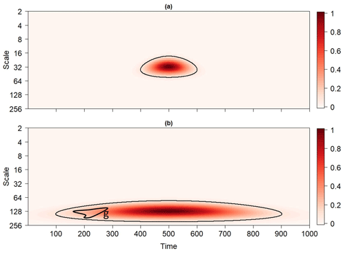
Figure 1 The normalized reproducing kernel of the Morlet wavelet dilated and translated to (a) (500, 32) and (b) (500, 128). Contours enclose the regions in the timescale plane where the normalized reproducing kernel exceeds 0.1. The closed path g in Fig. 1b can be continuously deformed into a point so that it does not surround a hole in the contoured region.

2.2 Statistical significance tests

2.2.1 Point-wise significance

In point-wise significance testing, one individually compares a wavelet quantity at every point in H to the critical level of the point-wise test, which depends on the chosen point-wise significance level α_pw and usually on the wavelet scale a. For wavelet power spectra of climate time series, point-wise test critical values are often determined from a theoretical red-noise background (Torrence and Comp, 1998). For wavelet coherence, partial coherence, multiple coherence, and auto-bicoherence, Monte Carlo methods need to be implemented to estimate the critical values (Grinsted et al., 2004; Ng and Chan, 2012; Hu and Si, 2016; Schulte, 2016b). However, a parametric bootstrap method may be required for determining the critical values of an arbitrary background model if analytical background models are not readily available (Maraun et al., 2007). Using the point-wise test, one assigns to each point in H a p value, ρ_pw, representing the probability of finding the observed or more extreme wavelet quantity (power, coherence, etc.) when the null hypothesis is true. The result of the point-wise test is the subset

$$\begin{array}{}\text{(4)}& P_{\mathrm{pw}}=\left\{\left(b,a\right):{\mathit{\rho }}_{\mathrm{pw}}\left(b,a\right)<{\mathit{\alpha }}_{\mathrm{pw}}\right\},\end{array}$$

of H, representing regions where point-wise significant wavelet quantities have been identified.

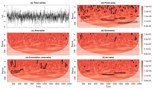
Figure 2 (a) A realization of a red-noise process (denoted by R(t)) with lag-1 autocorrelation coefficient equal to 0.4 together with its rectified wavelet power spectrum after the application of the (b) point-wise, (c) area-wise, (d) geometric, (e) cumulative area-wise, and (f) cumulative arc-wise tests. The point-wise, cumulative arc-wise, and cumulative area-wise tests were applied at the 5 % significance levels. The geometric and area-wise tests were applied at the 0.01 level to 5 % point-wise significance regions. Contours enclose regions of statistical significance. Light shaded region represents the cone of influence where edge effects become important.

To better understand the utility of the point-wise testing procedure, consider two example time series, where the first time series, R(t), corresponds to a realization of a red-noise process with a lag-1 autocorrelation coefficient equal to 0.4 (Fig. 2a). The second time series, X(t), shown in Fig. 3a, is given as

$$\begin{array}{}\text{(5)}& X\left(t\right)=S\left(t\right)/{\mathit{\sigma }}_{\mathrm{s}}+N\left(t\right)/m{\mathit{\sigma }}_n,\end{array}$$

where

$$\begin{array}{}\text{(6)}& {\displaystyle }S\left(t\right)=\sum _{j=\mathrm{1}}^{\mathrm{3}}\sin {\displaystyle \frac{\mathrm{2}\mathit{\pi }}{{\mathrm{2}}^{j+\mathrm{5}}}}t+\mathit{\delta }\left(t\right),\text{(7)}& {\displaystyle }\mathit{\delta }\left(t\right)=\left\{\begin{array}{ll}\mathrm{60}& t=\mathrm{1000}\\ \mathrm{0}& \text{otherwise}\end{array}\right.,\end{array}$$

and N(t) is a realization of a red-noise process with a lag-1 autocorrelation coefficient equal to 0.1. The constants σ_s and σ_s are the standard deviations of S(t) and N(t), respectively. The real number m is a measure of the signal-to-noise ratio, with larger values indicating a relatively higher signal.

The outcomes of the point-wise test applied to the (rectified; Liu et al., 2007) wavelet power spectrum of X(t) and R(t) are shown in Figs. 2b and 3b. For R(t), the point-wise test applied at α_pw=0.05 identified many statistically significant wavelet power coefficients, all of which being spurious by construction. The spurious results are seen occurring in contiguous regions, and the union of all such regions is P_pw. For the wavelet power spectrum of X(t), statistically significant wavelet power at the periods 64, 128, and 256 is seen clustering in narrow bands, reflecting the periods of the individual sinusoids (Fig. 3b). The singularity at t=1000 emerges as a scale-elongated region of point-wise significance, extending from a period of 2 to a period of approximately 32. What about the other features seen in the wavelet power spectrum? All the other significance regions are spurious by construction because they are associated with the noise term N(t), implying that they resulted from stochastic fluctuations. Thus, without further investigation, it would be impossible to know without prior knowledge of X(t) if the features associated with N(t) are part of the signal or not. These examples highlight how the number of spurious results can be large and how they could impede the differentiation between an underlying signal and background noise. It is therefore important to reduce the number of spurious results using other statistical methods.

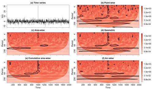
Figure 3 Same as Fig. 2, except for the ideal time series X(t) representing the linear superposition of three sinusoids with period equal 64, 128, and 256; a singularity at t=1000; and a realization of red-noise process with lag-1 autocorrelation coefficient equal to 0.1. The signal-to-noise ratio, m, is equal to 0.4.

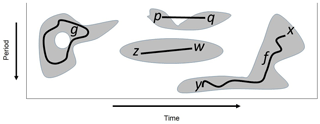
Figure 4 Four point-wise significance patches whose union is the set of all point-wise significant values. The closed path g encircles a hole, while the path f connects the points x and y belonging to the same path component or patch. The patch containing the points z and w is convex, contrasting with the patch containing the points p and q.

2.2.2 Area-wise and geometric testing

As noted by Maraun et al. (2007), the application of the point-wise test N_pw times will on average produce N_pwα_pw spurious results, with the spurious results occurring in clusters or patches. These so-called point-wise significance patches arise from the reproducing kernel of the analyzing wavelet that represents intrinsic correlations among wavelet coefficients. As noted by Schulte (2016a), patches can be rigorously defined using ideas from topology. That is, a patch is a path-connected component of P_pw, where a path-connected component is an equivalent class of P_pw resulting from an equivalence relation ∼ on P_pw that makes points $x,y\in P_{\mathrm{pw}}$ equivalent (written x∼y) if they can be connected by a continuous path $f:\left[\mathrm{0}\mathrm{1}\right]\to P_{\mathrm{pw}}$ such that f(0)=x and f(1)=y (Fig. 4). The equivalence relation ∼ reduces the original large set of points in P_pw to a smaller set of patches; the implications of which will be described later.

Because patches arise from the reproducing kernel, patches inherit the geometric characteristics of the reproducing kernel, such as convexity, area, length, and width. As an example, consider the set shown in Fig. 1b entirely consisting of points enclosed by the thick black contour. The contoured region is a subset of H for which the normalized reproducing kernel dilated and translated to (500, 128) exceeds 0.1. The set is convex (i.e., contains no concavities) because any two points in it can be connected by a line that remains entirely in the set (Fig. 4). The convexity of the set suggests that typical patches will be convex, which can be confirmed by generating a large ensemble of patches found in the wavelet power spectra of realizations of a red-noise process (Schulte et al., 2015). The convexity of patches plays an important role in understanding how different statistical tests perform. Another important geometric property is area, which reflects the dilated reproducing kernel so that patches at greater scales will be generally larger than those located at smaller scales, as Fig. 1 suggests.

Recognizing that a typical patch area is given by the reproducing kernel, Maraun et al. (2007) developed an area-wise test, which is conducted as follows. First choose a critical area P_crit(b,a) defined as a subset of H for which the reproducing kernel dilated and translated to (b, a) exceeds a certain critical level K_crit. That is,

$$\begin{array}{}\text{(8)}& P_{\mathrm{crit}}\left(b,a\right)=\left\{\left(b{}^{\prime },a{}^{\prime }\right)\mathrm{|}K\left(b,a;b{}^{\prime },a{}^{\prime }\right)>K_{\mathrm{crit}}\right\}.\end{array}$$

The set of points whose associated wavelet quantities are also area-wise significant is then the set

$$\begin{array}{}\text{(9)}& P_{\mathrm{aw}}=\bigcup _{P_{\mathrm{crit}}\left(b,a\right)\subset P_{\mathrm{pw}}}{P}_{\mathrm{crit}}\left(b,a\right),\end{array}$$

representing the union of all critical areas that lay completely inside P_pw. The larger the critical area, the larger a patch needs to be for it to be deemed area-wise significant so that P_crit(b,a) is related to α_aw, the significance level of the area-wise test. As discussed by Maraun et al. (2007), the critical area that corresponds to α_aw is determined using a root-finding algorithm, which is a non-trivial step that can be circumvented by performing a geometric test instead, as discussed below.

While the area-wise test effectively addresses the multiple-testing pitfall of the point-wise test, the use of the root-finding algorithm renders the practical implementation of the test difficult. To overcome this drawback, Schulte et al. (2015) constructed a geometric test whose test statistic is normalized area, which is defined as the patch area, A_patch, divided by the square of the patch's mean scale coordinate, $\widehat{a}$. That is,

$$\begin{array}{}\text{(10)}& A_{\mathrm{norm}}={\displaystyle \frac{A_{\mathrm{patch}}}{{\widehat{a}}^{\mathrm{2}}}},\end{array}$$

where the division by the mean scale coordinate accounts for how the reproducing kernel results in the scale-dependent expansion of patches in the time and scale direction. Thus, the normalized areas of patches can be readily compared regardless of where the patches are in H. The critical value of this test is assessed using Monte Carlo methods as follows: (1) generate wavelet spectra under some null hypothesis (e.g., red noise), (2) create a null distribution of normalized area using the patches found in the wavelet spectra, and (3) estimate the critical level of the test corresponding to the geometric significance level α_geo by computing the percentile of the null distribution corresponding to 1-α_geo. This null distribution calculation can be performed rapidly because wavelet spectra often contain many patches. However, for wavelet coherence, Monte Carlo methods must be applied twice because the critical levels of the point-wise test must be also empirically estimated. Fortunately, the length of the noise realizations needed to generate the null distribution of normalized areas need not be the same length of the input time series because the patch area is unrelated to the time series length; it is related to the reproducing kernel. As such, the realizations can be of shorter length, improving the efficiency of the null distribution computation. The ability to efficiently generate a null distribution allows p values associated with the geometric test to be further adjusted to account for multiple testing. For example, the false discovery rate of the geometric test can be controlled at a desired level if the number of patches to which the test is applied is large (Schulte et al., 2015).

It is important to note that the geometric and area-wise tests differ in the way they assign statistical significance to points. For the geometric test, all points in a patch will be deemed insignificant or significant if the patch is deemed statistically insignificant or significant. However, strictly speaking, the area-wise test evaluates the statistical significance of wavelet quantities associated with points in P_pw based on the geometric properties of the path-connected subsets of P_pw to which they belong. That is, for a wavelet quantity at (b, a) to be area-wise significant means that there must be a P⊆P_pw containing (b, a) that is path-connected, sufficiently convex, and large enough to have $P_{\mathrm{crit}}\left(b,a\right)\subset P$. If P is a patch, then no subset of P can be area-wise significant if P is not, consistent with the patch-sorting interpretation. On the other hand, P may contain both area-wise and non-area-wise significant subsets, opposing the patch-sorting interpretation. As discussed earlier, the equivalent relation ∼ reduces the initial large set of points to a set of fewer patches, implying that the number of spurious results arising from the geometric and area-wise test is less than that of the point-wise test.

Figures 2 and 3 show the wavelet power spectra of X(t) and R(t) after the application of the area-wise and geometric tests at the 0.1 significance level, where the area-wise test was performed using an existing R software package (available at https://rdrr.io/github/Dasonk/SOWAS/, last access: 12 January 2018). Both tests are seen reducing the number of spurious results arising from the point-wise significance test applied at the α_pw=0.05 level. However, as shown in Fig. 3c, the area-wise test also deems features associated with the signal S(t) to be noise. For example, the patch located at a period of 256 extending from t=100 to t=1700 is no longer statistically significant. Note also that the area-wise test largely filters out the scale-elongated feature associated with the singularity of X(t) at t=1000, while the geometric test deems the feature to be statistically significant. This difference in performance is expected because patches must be long with respect to the reproducing kernel to be area-wise significant, whereas there is no such constraint for the geometric test. Thus, the area-wise test is better suited for situations in which only periodicities are sought because periodicities induce temporally long patches. In general, the area-wise and geometric tests will reduce the signal detected by the point-wise test because the area-wise and geometric tests are theoretically constrained to detect a smaller amount of signal than the point-wise test (Table A1). This theoretical constraint raises a natural question: can a test simultaneously reduce statistical artifacts and increase signal detection (true positive results) relative to the point-wise test? The fact that patches enlarge with increasing α_pw suggests that examining the areas of patches across a set of point-wise significance levels could improve signal detection relative to the point-wise test.

2.2.3 Cumulative area-wise testing

Maraun et al. (2007) and Schulte et al. (2015) demonstrated that the area-wise and geometric tests are procedures for reducing the number of spurious results. However, both tests suffer from the drawback of having to select both an area-wise (or geometric) significance level and a point-wise significance level. This dual significance level selection is a cause for concern because a single wavelet quantity can have different levels of area-wise or geometric significance depending on the chosen point-wise significance level, leading to uncertainty as to whether the wavelet quantity is statistically artificial or distinguishable from background noise.

To address this concern, Schulte (2016a) suggested that changes in the geometric and topological characteristics of patches should be assessed over a finite set of point-wise significance levels ${\mathit{\alpha }}_{\mathrm{1}},{\mathit{\alpha }}_{\mathrm{2}},\mathrm{\dots },{\mathit{\alpha }}_N$. If the point-wise significance levels ${\mathit{\alpha }}_{\mathrm{1}},{\mathit{\alpha }}_{\mathrm{2}},\mathrm{\dots },{\mathit{\alpha }}_N$ are chosen such that

$$\begin{array}{}\text{(11)}& {\mathit{\alpha }}_{\mathrm{1}}<{\mathit{\alpha }}_{\mathrm{2}}<\mathrm{\dots }<{\mathit{\alpha }}_{\mathrm{N}},\end{array}$$

then the sets

$$\begin{array}{}\text{(12)}& P_{\mathrm{pw}}^i=\left\{\left(b,a\right):{\mathit{\rho }}_{\mathrm{pw}}\left(b,a\right)<{\mathit{\alpha }}_i\right\},\end{array}$$

will form a filtration

$$\begin{array}{}\text{(13)}& \mathit{\varnothing }=P_{\mathrm{pw}}^{\mathrm{1}}\subseteq P_{\mathrm{pw}}^{\mathrm{2}}\subseteq \mathrm{\dots }\subseteq P_{\mathrm{pw}}^N=H,\end{array}$$

of H for a sufficiently small α₁ and large α_N value. Equation (13) expresses the intuitive idea that one can start with an empty set (no statistically significant wavelet quantities) and build the complete timescale plane by increasing the point-wise significance level to a value that renders all wavelet quantities statistically significant.

An idealized example of a wavelet domain filtration is shown in Fig. 5a. The application of the point-wise test at the α₁ level results in no statistically significant regions, whereas the application of the test at α₂ results in a relatively small region of point-wise significance (dark gray). In contrast, setting the point-wise significance level to α₅ results in nearly all wavelet quantities being statistically significant, as indicated by the light gray region. At α₆, all wavelet quantities are statistically significant, and $P_{\mathrm{pw}}^{\mathrm{6}}$ is H.

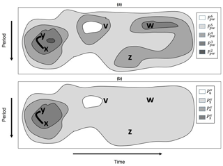
Figure 5 (a) An idealized example of a timescale plane filtration and (b) a geometric pathway corresponding to the point x and the filtration shown in (a). The first two members of the geometric pathway shown in (a) are the empty set and are not shown.

Although filtrations like Eq. (13) have proven to be useful in a data analysis method called persistent homology (Edelsbrunner and Harer, 2008), this method focuses on the sets of all point-wise significant values. At present, the concern is the statistical significance of a wavelet quantity at a point, and thus a more local approach is needed, though the utility of Eq. (13) will become more apparent in Sect. 2.2.5. To localize the persistence approach, a local filtration about x called a geometric pathway is needed (Schulte, 2016a). Mathematically, a geometric pathway G_x corresponding to a point x is a nested sequence

$$\begin{array}{}\text{(14)}& \mathit{\varnothing }=P_{\mathrm{1}}^x\subseteq P_{\mathrm{2}}^x\subseteq \mathrm{\dots }\subseteq P_N^x=H,\end{array}$$

where

$$\begin{array}{}\text{(15)}& P_i^x=\left\{\left(b,a\right):\left(b,a\right)\in P_{\mathrm{pw}}^i,\left(b,a\right)\sim x\right\}.\end{array}$$

A concrete example of a geometric pathway G_x is shown in Fig. 5b, where the geometric pathway corresponds to the wavelet domain filtration shown in Fig. 5a. In this example, $P_{\mathrm{1}}^x=\mathit{\varnothing }$ and $P_{\mathrm{2}}^x=\mathit{\varnothing }$, where $P_{\mathrm{2}}^x=\mathit{\varnothing }$ because x is not in the dark gray region shown in Fig. 5a representing $P_{\mathrm{pw}}^{\mathrm{2}}$. Although the set $P_{\mathrm{pw}}^{\mathrm{3}}$ comprises two path components or patches, only the component containing both x and y corresponds to the geometric pathway member at α₃. The reason is because any point equivalent to w is not equivalent to x on $P_{\mathrm{pw}}^{\mathrm{3}}$, as those points cannot be connected to x by a path fully contained in $P_{\mathrm{pw}}^{\mathrm{3}}$. Thus, in this example,

$$\begin{array}{}\text{(16)}& P_{\mathrm{3}}^x=\left\{\left(b,a\right):\left(b,a\right)\in P_{\mathrm{pw}}^{\mathrm{3}}\text{and}\left(b,a\right)\sim x\right\},\end{array}$$

$y\in P_{\mathrm{3}}^x,$ and $w\notin P_{\mathrm{3}}^x$. A similar situation occurs at α₄ because $P_{\mathrm{pw}}^{\mathrm{4}}$ has three path-connected components containing v, w, x, y, and z, but x is only equivalent to points that are equivalent to y. At α₅, the set $P_{\mathrm{pw}}^{\mathrm{5}}$ is path-connected ($x\sim y\sim z\sim v\sim w$) and is thus the fifth member of G_x. The sixth and last member of G_x is H.

Using the definition of a geometric pathway, Schulte (2016a) constructed a cumulative area-wise test that assesses the statistical significance of wavelet quantities by associating, to each point x in H, the total normalized area integrated over its geometric pathway G_x. The first step of the procedure is to calculate the normalized areas $A_{\mathrm{1}}^x,A_{\mathrm{2}}^x,\mathrm{\dots },A_N^x$ corresponding to the N members of G_x, where $A_i^x$ is assumed to be zero if $P_i^x=\mathit{\varnothing }$ or $P_i^x=\left\{x\right\}$. The second step is to compute the sum,

$$\begin{array}{}\text{(17)}& A^x=\sum _{k=\mathrm{1}}^N{A}_k^x,\end{array}$$

and compare A^x to a critical area A_crit determined by Monte Carlo methods. In the Monte Carlo approach, wavelet spectra and corresponding geometric pathways are generated under some null hypothesis, and a null distribution is calculated from all the computed total normalized areas. The critical area corresponding to the α_c level of the test is the percentile of the null distribution corresponding to 1-α_c. Performing these steps for all x∈H results in an adjusted p value at every point that accounts for multiple testing and the correlation among adjacent wavelet coefficients. As noted by Schulte (2016a), the computational efficiency of the cumulative area-wise test can be improved by setting α₁=0.02 and α_N=0.18, though this selection means that the cumulative area-wise test may no longer adjust p values at every point in H because complete filtrations like Eq. (13) may no longer be under consideration. Nevertheless, using a limited range of point-wise significance levels generally results in a better performance of the cumulative area-wise test relative to the geometric test performed at a single point-wise significance level (Appendix A and Table A1).

A disadvantage of the cumulative area-wise testing procedure is that it involves the computation of nested sequences, which renders the test computationally inefficient for long time series. Fortunately, the computation of nested sequences can be avoided as follows. First note that the test statistic for the cumulative area-wise test can be replaced by the mean normalized area without changing the outcome of the test. The criterion for a point to be cumulative area-wise significant is then

$$\begin{array}{}\text{(18)}& {\widehat{A}}^x={\displaystyle \frac{\mathrm{1}}{N}}\sum _{k=\mathrm{1}}^N{A}_k^x>{\widehat{A}}_{\mathrm{Crit}},\end{array}$$

where ${\widehat{A}}_{\mathrm{Crit}}$ is the critical level of the test calculated by computing the percentile of the null distribution comprising mean normalized areas corresponding to 1−α_c. Furthermore, there is a one-to-one relationship between the normalized area of a patch and its geometric test p value because a greater normalized area always means a lower p value. Thus, if ${\mathit{\rho }}_i^x$ is the p value associated with $A_i^x$, then the criterion for a wavelet quantity to be cumulative area-wise significant is

$$\begin{array}{}\text{(19)}& {\widehat{\mathit{\rho }}}^x={\displaystyle \frac{\mathrm{1}}{N}}\sum _{k=\mathrm{1}}^N{\mathit{\rho }}_k^x<{\mathit{\alpha }}_{\mathrm{c}},\end{array}$$

because there is also a one-to-one relationship between α_c and the critical level of the test. Equation (19) implies that to perform the cumulative area-wise test, one can individually perform the geometric test at each point-wise significance level and then compute ${\widehat{\mathit{\rho }}}^x$, avoiding the computation of nested sequences as in the original formulation of the cumulative area-wise test.

This interpretation of the cumulative area-wise test also allows the testing method to be put in an ensemble forecasting framework. That is, the individual geometric test p values are identified as ensemble members estimating the statistical significance of a wavelet quantity. The mean p value is identified with the ensemble mean that smooths out the unpredictable aspects of the forecast. In the present context, ${\widehat{\mathit{\rho }}}^x$ smooths out the features in the wavelet spectra resulting from noise and leaves the features that most of the geometric tests agree to be significant. This smoothing results in the suppression of noise but enhancement of the signal, which is consistent with how Schulte (2016a) found the cumulative area-wise test to perform superiorly to the geometric test in terms of signal detection, at least for periodic signals (Appendix A and Table A1).

Using Eq. (19), we now devise a simplified approach to the cumulative area-wise test. In the simplified approach, all points in H are initially assigned a value of 0. Then, for a fixed point-wise significance level, the geometric test is performed on all patches. The points falling in those patches that are geometrically significant at the α_c level are then assigned the value 2. The values for the points not in geometrically significant patches are left unchanged. This assignment step is then repeated for each point-wise significance level, and the values are stored separately so that each point in H is assigned a set of values, the number of values equaling the number of point-wise significance levels used to implement the cumulative area-wise test. Then, the average value at each point is computed, with regions where the average value exceeds unity deemed to be cumulative area-wise significant.

The application of the simplified cumulative area-wise test to the wavelet power spectra of R(t) and X(t) (Figs. 2e and 3e) reveals that the test is effective at reducing the number of spurious results arising from the point-wise test when applied at the α_c=0.05 level. Like the area-wise test, the reduction in spurious features is accompanied by a loss in signal detection. For example, the cumulative area-wise test, like the area-wise test, deems the wavelet power associated with the point-wise patch located at a period of 256 extending from t=100 to t=1700 in Fig. 3b to be statistically insignificant. On the other hand, the scale-elongated feature associated with the singularity of X(t) at t=1000 more clearly emerges from the application of the cumulative area-wise test than the area-wise test, which is not surprising because the cumulative area-wise test assesses statistical significance based on area without regard to the specific shape of patches.

Although this example suggests that the point-wise test detects a higher amount of signal than the cumulative area-wise test, a simplified experiment in Appendix A revealed that the simplified cumulative area-wise test can detect a higher amount of signal than the point-wise test when the signal-to-noise ratio is relatively high (Table A1). At low point-wise significance levels, the tests were found to detect a similar amount of the signal on average. Thus, a key strength of the cumulative area-wise test is that it can retain the signal while also reducing the number of spurious results arising from the point-wise test.

2.2.4 Cumulative arc-wise testing

While the area-wise, geometric, and cumulative area-wise tests can effectively reduce the number of spurious results, they do not test for the existence of periodicities embedded in a time series. This deficiency is especially true for the geometric and cumulative area-wise tests because they only consider the area of patches in the assessment of statistical significance. For example, the cumulative area-wise test can identify features that are long in scale but short in time as statistically significant (Fig. 3e). Thus, a new test needs to be constructed that is specifically designed to distinguish randomly stable fluctuations from those that are periodicities. As periodicities are determined by patch length, a strict test for periodicities should consider patch length and not patch area.

Using the idea that patch length is more closely linked to the presence of periodicities, we construct a cumulative arc-wise test that can be implemented using the following steps. For Step 1, fix a scale and point-wise significance level and identify point-wise significance arcs, where point-wise significance arcs are contiguous strings of points whose associated wavelet quantities are point-wise significant. Step 2 is to compute normalized arclength, defined as the number of points composing each arc divided by the scale in question. Step 3 is to repeat Steps 1 and 2 for all wavelet scales associated with the wavelet spectrum in question. Repeating the procedure for a finite set of point-wise significance levels allows for the assignment of total arclength to each point in the timescale plane. The null distribution can be computed using the Monte Carlo approach adopted for the cumulative area-wise test.

The application of the cumulative arc-wise test at the 0.05 significance level to the wavelet power spectra of X(t) and R(t) is shown in Figs. 2f and 3f, where point-wise significance levels ranging from 0.02 to 0.18 were used. The discrete spacing between adjacent point-wise significance was set to 0.02 to be consistent with the cumulative area-wise test applied earlier (Figs. 2e and 3e). Like with the other statistical tests, the number of spurious point-wise test results for both time series is seen as being dramatically reduced. For X(t), much of the signal detected by the point-wise test remains despite the greater stringency of the cumulative arc-wise test. A comparison of Fig. 3c and f reveals that the geometric and cumulative arc-wise tests detect a similar amount of the signal associated with the three sinusoids. As expected, the cumulative arc-wise test, like the area-wise test, largely filters out the scale-elongated feature shown in Fig. 3b, supporting the idea that both the arc-wise and area-wise tests should be preferred to the geometric and cumulative area-wise tests in situations in which features associated with periodic signals are sought. In fact, in Appendix A it is shown that the cumulative arc-wise test can detect a higher amount of signal than the point-wise test for high signal-to-noise ratios.

2.2.5 Topological significance testing

A common theme among all the statistical procedures discussed so far is that they evaluate the statistical significance of wavelet quantities based on the geometric properties of the patches to which the corresponding points belong. However, as demonstrated by Schulte et al. (2015), topological properties are also important to statistical hypothesis testing. How do topological properties differ from geometric ones? Topological properties of an object are those that remain unchanged no matter how much the object is twisted or bent. Using topological characteristics of point-wise significance regions, additional information about the time series in question can be gained.

The basic principal behind topological significance testing is that topologically equivalent (that is, homeomorphic) objects have identical topological invariants (Ferri, 2017). In the present context, the object of interest is P_pw and the topological invariants of concern are the 0- and 1-D Betti numbers denoted by β₀ and β₁, respectively. The invariant β₀ measures the number of path components or patches composing P_pw, whereas β₁ measures the number of 1-D holes in P_pw. A region in P_pw has a hole if there is a closed path in it such that the path cannot be continuously deformed into a point (Fig. 4). Equivalently, holes are regions in H fully surrounded by points in P_pw. Although counter-intuitive, Schulte et al. (2015) showed that the presence of these holes is related to the statistical significance of the patch to which they correspond. To better understand how these holes are related to statistical significance, consider the reproducing kernel shown in Fig. 1b together with the set of points enclosed by the black contour. As shown in Fig. 1b, the closed path, g, in the contoured region can be continuously (e.g., no tearing or cutting) deformed into a point within the set by contracting or shrinking it, with this property holding for any closed path so that the set enclosed by the contour has no holes. As patches arise from the reproducing kernel, typical patches arising from isolated fluctuations will tend not to have holes at low point-wise significance levels. However, if two fluctuations are located at nearby frequencies and times, then the resulting patches in the wavelet power spectrum may contain holes (Schulte et al., 2015).

Using Betti numbers, one can assess whether P_pw is homeomorphic to $P_{\mathrm{noise}}=\left\{\left(b,a\right):{\mathit{\rho }}_{\mathrm{noise}}\left(b,a\right)<{\mathit{\alpha }}_{\mathrm{pw}}\right\}$, where ρ_noise denotes the p value resulting from the application of the point-wise test to a noise spectrum such as the wavelet power spectrum associated with a realization of a red-noise process or the coherence spectrum associated with a pair of red-noise realizations. More specifically, a topological significance test is performed as follows: (1) compute wavelet spectra under some noise model, (2) compute P_noise for each of the wavelet spectra, and (3) compute the null distribution of β₀ and β₁. The critical values associated with the two-sided topological significance test applied at the α_topo significance level are the percentiles of the null distribution corresponding to 1-α_topo∕2 and α_topo∕2. The two-sided test accounts for how the number of patches or holes can be unusually high or low relative to noise. However, as shown by Schulte et al. (2015), a typical patch found in the wavelet power spectrum of red noise will typically have no holes at point-wise significance levels less than 0.2, suggesting that a one-sided topological test may be better than a two-sided test at low point-wise significance levels.

Topological equivalence at a single point-wise significance does not necessarily mean that the time series in question is topological indistinguishable from background noise. That is, the result of the topological significance test may be sensitive to the chosen point-wise significance level. To address this concern, it is necessary to adopt the persistent homology approach (Edelsbrunner and Harer, 2008) in which a topological space is distinguished from another topological space homeomorphic to it through an examination of filtered versions of the spaces (Ferri, 2017). In the wavelet analysis context, the spaces are the timescale planes associated with noise and the times series in question, which are rectangular and topological equivalent. To distinguish the timescale planes, it is necessary to examine the filtered versions of the timescale planes using the filtration represented by Eq. (13). Computing β_o and β₁ at each step in the filtration results in 0- and 1-D persistent homology profiles (PHPs; Qaiser et al., 2016). The more comprehensive topological significance then involves comparing PHPs for a time series in question to that of noise by applying the topological significance test at each point-wise significance level.

The utility of the topological significance testing procedure is demonstrated using the wavelet power spectra of X(t) and R(t). The 1-D PHP corresponding to R(t), shown in Fig. 6a, indicates that β₁ is maximum at α_pw=0.7 and decreases rapidly until reaching 0 at α_pw=0.1. The overall curve is the same for realizations of a red-noise process with any lag-1 autocorrelation coefficient, though the number of holes is greater for larger lag-1 autocorrelation coefficients (not shown). The 1-D PHP for X(t) is like that of R(t), suggesting that these time series are topologically indistinguishable. The application of the topological significance test with α_topo=0.05 further supports the topological equivalence of X(t) with red noise because the PHP associated with X(t) falls in the gray-shaded envelope representing the test non-rejection region, where the non-rejection region was obtained by generating 100 PHPs associated with 100 realizations of a red-noise process with a lag-1 autocorrelation coefficient equal to that of X(t). However, X(t) is not noise by construction, and thus the similarity of 1-D PHPs does not exclude the possibility that time series under consideration are indistinguishable from noise.

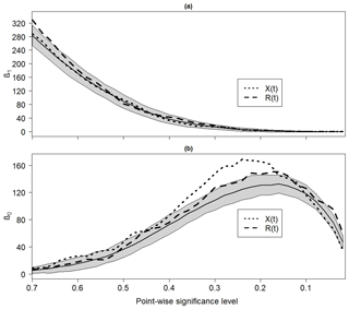
Figure 6 (a) The 1-D and (b) 0-D persistent homology profiles associated with R(t) and X(t). Gray shaded region is the non-rejection region of the topological significance test applied at the 0.05 significance level. The non-rejection region was calculated by generating 100 realizations of a red-noise process with lag-1 autocorrelation equal to 0.1, the lag-1 autocorrelation coefficient corresponding to X(t).

In contrast to the 1-D PHPs, the 0-D PHPs for X(t) and R(t) differ substantially (Fig. 6b). The PHP for X(t) is seen to reach a global maximum around α_pw=0.25, while the one for R(t) peaks around α_pw=0.18. The application of the topological significance test at the 0.05 level strongly supports the idea that X(t) is distinguishable from noise because β₀ far exceeds the critical level of the test at α_pw=0.25. Thus, there are features that are distinguishable from the background noise. These features are precisely those identified from the area-wise, geometric, cumulative arc-wise, and cumulative area-wise tests.

3 Practical applications to the Indian monsoon

3.1 Data

To understand the temporal behavior and spatial variability of Indian rainfall, monthly rainfall data for five homogenous regions (Parthasarathy et al., 1994) extracted from Indian Institute of Tropical Meteorology website (https://www.tropmet.res.in/Data Archival-51-Page, last access: 15 March 2019) were analyzed. The five divisions called the Peninsula, Northwest, Northeast, Central Northeast, and West Central regions were devised based on continuity of area, contribution to annual amount, and global and regional circulation parameters (Parthasarathy et al., 1994; Azad et al., 2010). The rainfall data for each region were obtained by area-weighted averaging the sub-divisional data corresponding to the meteorological subdivisions composing the homogenous region, where the sub-divisional data were obtained by averaging the rainfall data associated with representative rainfall gauges. An all-India (Parthasarathy et al., 1995) rainfall time series was also examined, as it is commonly reported in the literature. The monthly all-India rainfall time series is constructed by averaging the sub-divisional data after assigning a weight to each sub-division, which is determined by the sub-divisional area (Parthasarathy et al., 1994). These rainfall data span the long time period from 1871 to 2016 and are continuous, making them well-suited for a wavelet analysis. Each rainfall time series was converted into an anomaly time series by subtracting the 1871–2016 mean for each month from the individual monthly values. After the conversion to an anomaly time series, the time series were standardized by dividing them by their respective 1871–2016 standard deviations. The resulting time series are shown in Fig. 7.

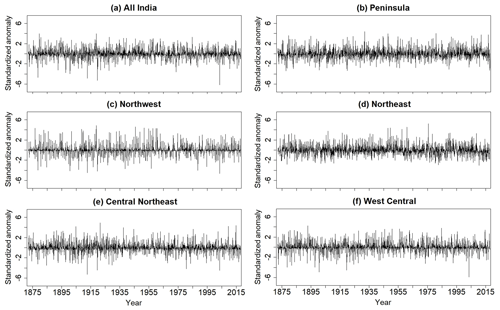
Figure 7 Standardized (a) all-India, (b) Peninsula, (c) Northwest, (d) Northeast, (e) Central Northeast, and (f) West Central rainfall time series.

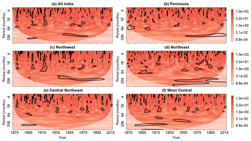
Figure 8 Wavelet power spectra of the standardized (a) all-India, (b) Peninsula, (c) Northwest, (d) Northeast, (e) Central Northeast, and (f) West Central rainfall time series after the application of the point-wise test at the 0.05 significance level. Contours enclose regions of statistical significance, and the light shaded region represents the cone of influence where edge effects become important.

The monthly Niño 3.4 index (available at https://www.esrl.noaa.gov/psd/gcos_wgsp/Timeseries/Data/nino34.long.data, last access: 15 March 2019) from 1871 to 2016 was used to characterize the state of the ENSO system. The Niño 3.4 index is defined as the average SST in the region bounded by 5^∘ N and 5^∘ S and by 170 and 120^∘ W. The seasonal cycle was removed from this time series in the same way as it was removed from the rainfall time series.

3.2 Wavelet power spectrum

The wavelet power spectra corresponding to the rainfall time series are shown in Fig. 8, where α_pw=0.05 in this case. Statistically significant features are seen for all six time series, with a large swath of point-wise significance being seen around a period of 256 months for the Peninsula, Northeast, and Northwest time series after 1950. For all the time series, most of the point-wise significance patches are seen as being located at lower periods and appear to have varying geometries. For example, the wavelet power spectrum for the Northwest time series contains a scale-elongated significance patch at around 1920, extending from a period of 4 months to a period of 64 months. A similar but less prominent feature is also evident in the wavelet power spectrum of all-India rainfall. For the remaining time series, no such features are readily identifiable from an inspection of the wavelet power spectra.

To account for how spurious results may result from multiple testing, the cumulative area-wise test was applied at the α_c=0.05 level to the wavelet power spectrum shown in Fig. 8. For these cases, the simplified cumulative area-wise test was applied using point-wise significance levels ranging from 0.02 to 0.18, with the spacing between adjacent point-wise levels equaling 0.02. Like with the point-wise test, statistically significant wavelet power is located around a period of 256 months for the Northwest and Northeast regions, raising the possibility that these time series contain periodicities at that timescale (Fig. 9). For all the time series, most of the statistically significant results are seen at periods less than 64 months. Two of the most prominent features are the scale-elongated significance patches around 1920 in the all-India and Northwest wavelet power spectra. Because the wavelet power associated with these scale-elongated features remain statistically significant after the application of the cumulative area-wise, there is strong evidence that the corresponding fluctuations exceed the red-noise background.

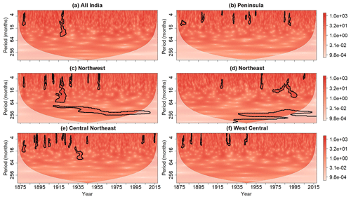
Figure 9 Same as Fig. 8 but after the application of the cumulative area-wise test at the 0.05 significance level.

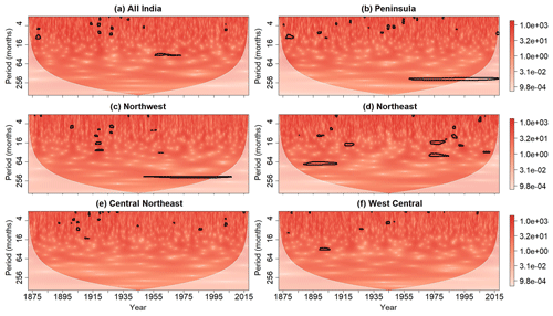
Figure 10 Same as Fig. 8 but after the application of the cumulative arc-wise test at the 0.05 significance level.

To better differentiate patches arising from singularities from those associated with periodicities, the cumulative arc-wise test was applied to wavelet power spectra shown in Fig. 8 at the same point-wise significance levels used for the cumulative area-wise test. As shown in Fig. 10, the application of the cumulative arc-wise test at the 5 % significance level reveals two time-elongated regions of statistical significance around a period of 256 months in the Peninsula and Northwest wavelet power spectra. However, the wavelet power around a period of 256 months is no longer statistically significant for the Northeast time series, suggesting that the point-wise significant wavelet power at that period is associated with a randomly stable oscillation. The scale-elongated features for the all-India and Northwest power spectra are largely filtered out like the scale-elongated features shown in Fig. 3 for X(t). This result suggests that the wavelet power at that time and at those periods is associated with a singularity-like time domain feature rather than a periodicity.

To gain a deeper understanding of the rainfall time series, the 0th and 1-D PHPs were computed for each time series. For clarity, we computed anomaly PHPs by subtracting the mean profile associated with noise from the individual profiles at each point-wise significance level. Thus, positive (negative) values mean that the number of patches (or holes) associated with the rainfall time series is greater (less) than that associated on average with noise. Because the lag-1 autocorrelation coefficients associated with each time series are nearly identical, a single test non-rejection region was computed using 100 realizations of a red-noise process with lag-1 autocorrelation coefficient equal to the mean lag-1 autocorrelation coefficient of the six rainfall time series. The mean noise profile was subtracted from both the upper and lower bounds of the test non-rejection region after the application of the topological significance test at the 0.05 level.

The 0th dimensional anomaly PHPs for each rainfall time series is shown in Fig. 11a. Many of the profiles are seen to deviate substantially from the mean noise profiles around α_pw=0.5 and α_pw=0.2. At around α_pw=0.5, the largest deviations are associated with the Northwest, West Central, and all-India time series. The profiles for the Northeast and Peninsula time series lay inside the confidence envelope so that those time series could be topologically indistinguishable from red noise. At around α_pw=0.15, the largest deviations are associated with the Northwest and Central Northeast profiles. The large deviations from the mean noise profile for the Northwest time series suggest that the statistically significant features identified by the cumulative area-wise test (Fig. 9) are unlikely statistical artifacts. On the other hand, the wavelet power spectrum of the West Central time series contains only five small regions of cumulative area-wise significance despite the large departures from the mean noise profiles at numerous point-wise significance levels. This finding raises the possibility of Type II errors for the cumulative area-wise test or a Type I error for the topological significance test.

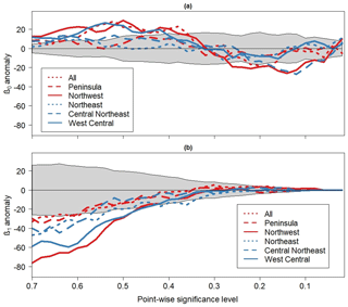
Figure 11 (a) The 0-D and (b) 1-D anomaly persistent homology profiles associated with the six rainfall time series. Gray shaded region is the non-rejection region of the topological significance test applied at the 0.05 significance level. The non-rejection region was calculated by generating 100 realizations of a red-noise process with lag-1 autocorrelation equal to the mean of all six lag-1 autocorrelation coefficients associated with the rainfall time series.

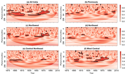
Figure 12 Wavelet coherence between Niño 3.4 index and time series of standardized (a) all-India, (b) Peninsula, (c) Northwest, (d) Northeast, (e) Central Northeast, and (f) West Central rainfall. Contours enclose regions where the wavelet coherence is cumulative arc-wise significant at the 0.05 level. For clarity, phase arrows representing the out-of-phase relationship between ENSO and rainfall are not displayed.

Additional insight into the time series is provided by the 1-D anomaly PHPs shown in Fig. 11b. In this case, all the rainfall time series appear to be topologically distinguishable from red noise for point-wise significance levels ranging from 0.7 to 0.65. Like with the 0th dimensional profiles, the departures are greatest for the Northwest and West Central time series, providing strong evidence that these time series comprise features exceeding background noise. For the West Central time series, the lack of arc-wise significance shown in Fig. 10 suggests that the topological significance cannot be attributed to periodicities with high confidence. For the Northwest time series, the cumulative area-wise test results suggest that topological significance may be attributed to the scale-elongated feature around 1915 and the enhanced wavelet power around a period of 256 months. The PHPs for all the time series converge to 0 below the point-wise significance level 0.3, and the lack of 1-D holes below 0.1 renders the isolation of topologically significant regions in H using the approach of Schulte et al. (2015) that determines where there is enhanced topological significance based on the location of holes difficult. However, for the Northwest time series, a few holes were identified at point-wise significance below 0.1 around the scale-elongated patches shown in Fig. 9c, supporting the results of the cumulative area-wise test.

3.3 Wavelet coherence

To determine the timescales at which ENSO influences on Indian rainfall are strongest, wavelet coherence was computed between the Niño 3.4 index and the rainfall time series for each region. The point-wise, cumulative area-wise, and cumulative arc-wise tests were applied to the wavelet coherence spectra at the 5 % significance level, but only the results for the cumulative arc-wise test are shown for brevity. The reason why the results for the cumulative arc-wise test are emphasized is that we are interested in distinguishing non-random coherent oscillations at a scale from randomly stable covarying oscillations.

The results for the wavelet coherence analysis are shown in Fig. 12. Statistically significant wavelet coherence was identified for all six time series, but coherence between the Niño 3. 4 index and the time series of rainfall is seen to be most salient for the all-India, Northwest, and West Central regions. The statistically significant coherence is mainly confined to the period band of 16 to 64 months, and time periods of enhanced coherence appear to follow time periods of weak coherence. The results shown in Fig. 12 suggest that the 16-month to 64-month mode of SST variability across the Niño 3.4 region modulates Indian rainfall, which is a well-known idea (Torrence and Webster, 1999). It is also noted that the coherence between rainfall and the Niño 3.4 index varies spatially, consistent with recent work showing how ENSO influences are spatially non-uniform (Roy et al., 2017).

4 Summary and discussion

Wavelet analysis is a tool for extracting time-localized and scale-dependent features from time series. To assess the confidence with which features in wavelet spectra are distinguishable from a noise background, it is necessary to implement statistical significance tests. The traditional approach to statistical significance testing is to individually test whether a wavelet quantity associated with a point in the timescale plane exceeds a background noise spectrum. This point-wise approach has been applied in numerous papers since its first application to wavelet analysis by Torrence and Compo (1998).

Despite its wide use, the point-wise test suffers from two pitfalls, as noted by Maraun and Kurths (2004) and Maraun et al. (2007) and as shown in Fig. 2. The first pitfall is that the test typically produces many false positive results because of the simultaneous testing of multiple hypotheses. Secondly, spurious results occur in clusters, with the clusters reflecting the reproducing kernel of the analyzing wavelet. To remedy the pitfalls of the point-wise test, Maraun et al. (2004) developed an area-wise test to reduce the number of spurious point-wise significance patches based on the area and geometry of the patches. While the method has been shown to be effective at reducing the number of spurious results, the test is computationally inefficient. To address the concern of computational inefficiency, Schulte et al. (2015) proposed a geometric test that reduces the number of spurious results by assigning a normalized area to each patch. However, both the area-wise and geometric test suffer from a binary decision pitfall in which both an area-wise (or geometric) significance level and a point-wise significance level must be selected. This dual selection inevitably leads to uncertainty regarding the statistical significance of a wavelet quantity.

Schulte (2016a) developed a cumulative area-wise test to reduce the sensitivity to the chosen point-wise significance level. Adopting ideas from persistent homology, the test provides a way to assess the statistical significance of a wavelet quantity located at a point by examining how the area of a nested sequence of patches containing the point changes as the point-wise significance is changed. This test can be viewed as an ensemble technique, where the individual estimates of statistical significance are associated with the p values of the geometric tests performed at various point-wise significance levels. The ensemble mean is the mean of all such p values. Much like how the ensemble mean in weather forecasting filters out unpredictable aspects associated with the individual ensemble members, the cumulative area-wise test filters out the unpredictable aspects associated with a time series in question; the degree to which this occurs depends on the chosen cumulative area-wise significance level.

Strictly speaking, the geometric and cumulative area-wise tests (and to a lesser extent the area-wise test) do not assess the confidence with which periodicities are embedded in time series. To make such assessments, the temporal length of cross sections of point-wise significance patches needs to be computed and compared to a null distribution of cross section lengths. This procedure is termed the cumulative arc-wise test and is like the cumulative area-wise test. Two ideal cases showed that the procedure reduces the number of spurious results arising from the point-wise test while also detecting periodicities embedded in time series. The arc-wise test is also capable of eliminating scale-elongated point-wise significance features induced from singularities in the time domain. Thus, when testing for the presence of periodicities, the arc-wise test should be preferred to the cumulative area-wise and geometric tests because those tests are unable to distinguish features arising from singularities from those associated with periodicities. An additional benefit of the cumulative arc-wise test is that it operates in one dimension, rendering its implementation more rapid than that of the cumulative area-wise test.

The application of the statistical tests to the Indian rainfall time series further highlighted the benefits and disadvantages of the various methods. The application of the point-wise test to the wavelet power spectra of the Indian rainfall resulted in many statistically significant results. Much of the point-wise significant wavelet power was deemed indistinguishable from background noise after the implementation of the cumulative area-wise and arc-wise tests. However, for some Indian sub-regions, statistically significant features were identified. For example, the Northwest and all-India time series were found to contain features consistent with singularities.

The application of the cumulative arc-wise test to wavelet coherence revealed statistically significant coherence between rainfall for many of the subregions and the Niño 3.4 index at a period of 16 to 64 months. The most pronounced coherence was found between the all-India rainfall and Niño 3.4 index time series, while the weakest coherence was generally found for the Northeast region. These results highlight the spatial variability of the ENSO teleconnection. Periods of high coherence were found to be followed by periods of lower coherence, consistent with prior work showing how the Indian rainfall-ENSO teleconnection is non-stationary (Torrence and Webster, 1999).

Topological methods were also adopted to further assess whether the rainfall time series are consistent with a red-noise process. An examination of 0th dimensional PHPs showed that the all-India, Northwest, and West Central rainfall time series are topologically distinguishable from red noise. The 1th dimensional PHPs revealed that all rainfall time series are distinguishable from red noise despite the lack of cumulative arc-wise or area-wise significance in the corresponding wavelet power spectra. The discrepancies among the tests suggest that a further investigation is required.

Although only two ideal cases have been in the paper, additional ideal cases are presented in the Supplement for reference. The ideal cases include time series with a single sinusoid and a time series with a single singularity without periodic features. An R software package has been written by the author to implement the various tests documented in this paper. The software package can be found at http://justinschulte.com/wavelets/advbiwavelet.html (last access: 29 April 2019).

Appendix A

A simplified sinusoid experiment was conducted to assess how well the various statistical tests detect a periodic signal embedded in noise. In the experiment, time series of the form

$$\begin{array}{}\text{(A1)}& {\displaystyle }X\left(t\right)=\sin \mathrm{2}\mathit{\pi }/T/{\mathit{\sigma }}_{\mathrm{s}}+N\left(t\right)/m{\mathit{\sigma }}_n,\end{array}$$

were generated. In Eq. (A1), T=8 is the period of the sinusoid, σ_s is the standard deviation of the sinusoid, N(t) is a realization of a red-noise process, σ_n is the standard deviation of N(t), and m is a number representing the signal-to-noise ratio. In the experiment, 100 different realizations of X(t) were constructed by generating 100 realizations of N(t). The wavelet power spectrum of each realization of X(t) was computed. The computations were repeated for values of m ranging from 0.01 to 1.0. For each statistical test, the fraction of wavelet power coefficients statistically significant at a period of 8 was calculated for each realization. The mean fraction was then calculated for each value of m, resulting in a curve representing how much of the signal on average is detected for different signal-to-noise ratios. Values close to 1.0 indicate that the test performed well at detecting the periodic signal. For the experiments, the lag-1 autocorrelation coefficient was set to 0.1, 0.5, and 0.9, but only the results for 0.5 are displayed because the results are only weakly dependent on the lag-1 autocorrelation coefficient. The point-wise, cumulative area-wise, and cumulative arc-wise tests were applied at the 5 % level, and the geometric and area-wise tests were applied at the 10 % level to 5 % point-wise significance regions.

As shown in Table A1, the amount of the signal detected by any of the tests increases as the signal-to-noise increases. Despite how the cumulative area-wise test is more stringent than the point-wise test, the tests detected a comparable amount of the signal for low signal-to-noise ratios; for signal-to-noise ratios greater than 0.7, the test performed better. The cumulative arc-wise test outperformed the cumulative area-wise test for signal-to-noise ratios greater than 0.5. Consistent with theory, both the area-wise and geometric tests performed worse than the point-wise test. The performance of all tests was found to improve if the lag-1 autocorrelation coefficients were increased to 0.9 and was found to worsen if the lag-1 autocorrelation coefficient was set to 0.1.

Table A1 The fraction of wavelet power coefficients at a period of 8 that are statistically significant in the case of a sinusoid embedded in noise with varying signal-to-noise ratios.