Negentropy anomaly analysis of the borehole strain associated with the M_s 8.0 Wenchuan earthquake

A large earthquake of 8.0 magnitude occurred on 12 May 2008, 14:28 UTC, with the epicentre in Wenchuan. To investigate the pre-earthquake anomalous strain changes, negentropy is introduced to borehole strain data for three locations, approximated by skewness and kurtosis, revealing the non-Gaussianity of recorded fluctuations. We separate the negentropy anomalies from the background by Otsu's method and accumulate the anomaly frequency on different scales. The results show that the long-term cumulative frequency of negentropy anomalies follows a sigmoid behaviour, while the inflection point of the fitting curve is close to the occurrence of the earthquake. For the short-term analysis before the earthquake, there are two cumulative acceleration phases. To further verify the correlation with the earthquake, we compare our findings for different time periods and stations and rule out the possible influence of meteorological factors. We consider the negentropy analysis to exhibit potential for studying pre-earthquake anomalies.

1 Introduction

Changes in crustal deformation fields over time have been recorded at least for some large earthquakes (Thatcher and Matsuda, 1981), such as the 2011 Tōhoku earthquake (Hirose, 2011) and the Ruisui earthquake in Taiwan in 2013 (Canitano et al., 2015). Borehole strainmeters which detect the crustal changes provide an opportunity to investigate the preparation process prior to earthquakes. Many strain observations were of significance to research (Linde et al., 1996), although there were some unsuccessful detections, such as those of the 1987 Superstition Hills earthquake (Agnew and Wyatt, 1989), 1989 Loma Prieta earthquake (Johnson et al., 1990) and 2009 L'Aquila earthquake (Amoruso and Crescentini, 2010). Various methods are used in identifying borehole strain anomalies based on a large amount of monitoring data. Experienced scholars extract borehole strain anomalies by discriminating patterns of waveform behaviours compared to those during the normal stage (Johnston et al., 2006; Chi et al., 2014). In the time domain, Qiu et al. (2011) identified abnormal strain changes by the overrun rate and wavelet decomposition for the Wenchuan earthquake. While in the frequency domain, Qi and Jing (2011) thought that the signal with a period of 10 to 60 min might be anomalies through S transform compared with the background signal. In addition, statistical methods proved to be effective in distinguishing borehole strain anomalies with regard to large earthquakes, such as principal component analysis (Zhu et al., 2018) and correlation coefficients along with the consistency relation (Kong et al., 2018).

The probability density function (PDF) of observation data is also an informative way of extracting potential anomalies contained in earthquake generation processes. Manshour et al. (2009) extracted variance anomalies of the probability density of the Earth's vertical velocity increments and successfully found a pronounced transition from Gaussian to non-Gaussian prior to 12 moderate and large earthquakes. Before the Wenchuan earthquake, the high-frequency fluid observational data deviated from Gaussian distributions at 16 water level and 14 water temperature stations (Sun et al., 2016).

Rather than the whole PDF, its moments are often utilized; moments may be estimated quite reliably from relatively small amounts of data (Sattin et al., 2009). In 2016, Chen (2016) applied skewness and kurtosis (the third- and fourth-order moments) of the geoelectric data to pick up non-Gaussian distribution anomalies to predict impending large earthquakes in Taiwan. On the other hand, for turbulent or disordered systems, the non-Gaussian distribution of time series in the skewness–kurtosis domain attracts attention. Observation data series from various fields of geophysics indicate that a parabolic relation between skewness and kurtosis holds in fields such as seismology (Cristelli, 2012), oceanography (Sura and Sardeshmukh, 2012) and atmospheric science (Maurizi, 2006).

Thereby, it is possible that precursor anomalies lead to an increase in disordered components in observation data. Eftaxias et al. (2015) proved that the pre-catastrophic stage could break the persistency and high organization of the electromagnetic field through studying the fractional-Brownian-motion-type model using laboratory and field experimental electromagnetic data. In view of Lévy flight and Gaussian processes, the Lévy flight mechanism prevents the organization of the critical state being completed before earthquakes, since the long scales are cut off due to the Gaussian mechanism (Potirakis et al., 2019).

Entropy can serve as a measure of the unknown external energy flow into the seismic system (Akopian, 2015). Karamanos et al. (2005, 2006) quantified and visualized temporal changes of the complexity by approximate entropy; they claimed that significant complexity decrease and accession at the tail of the preseismic electromagnetic emission could be diagnostic tools for the impending earthquake. Approximate entropy has also been studied in catastrophic events (Nikolopoulos et al., 2004). Ohsawa (2018) detected earthquake activation precursors by studying the regional seismic information entropy on the earthquake catalogue.

Negentropy's definition is based on the entropy, and it is also widely used to detect non-Gaussian features. Yue et al. (2018) proposed a method for picking arrival time based on negentropy for microseismic data. In this study, the negentropy is applied to the borehole strain associated with the Wenchuan earthquake at the Guza station, approximated by skewness and kurtosis, which reveal the non-Gaussianity of borehole fluctuations. Subsequently we study the extracted negentropy anomalies on different scales to investigate correlations with crustal deformation. Furthermore, we did a comparison discussion for different time periods and stations.

2 Observation

YRY-4 borehole strainmeters, which are designed to record continuous deformation occurring over periods of minutes to years, have been deployed at depths of more than 40 m at more than 40 terrain-sensitive locations within China. These strainmeters are capable of resolving strain changes of less than one-billionth. The data sampling rate is once per minute.

The study period is from 1 January 2007 to 30 June 2009. The study area is shown in Fig. 1. We find that the Guza station stands on the southwestern end of the Longmenshan Fault zone. Besides this, the epicentre is about 150 km away from the station, which is within the monitoring capability of the borehole strainmeters (Su, 1991).

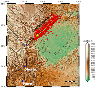
Figure 1 Location map showing the epicentre and three stations. The epicentre was located at 31.01^∘ N, 103.42^∘ E, shown by yellow star. The blue triangles show the strainmeter stations. The red circles are aftershock distribution from the main shock on 12 May to 30 October 2008. The green curve is the schematic curve of the main rupture zone, and black curves are faults.

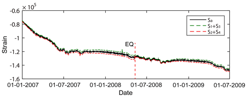
Because the four gauges of the YRY-4 borehole strainmeter are arranged at 45^∘ intervals, this design has improved its self-consistency. This arrangement produces four observation values: S_i, ($i=\mathrm{1},\mathrm{2},\mathrm{3},\mathrm{4}$) (Qiu et al., 2013). The self-consistency is shown in Eq. (1), which can be used to test the reliability of the data among the four gauges:

$$\begin{array}{}\text{(1)}& S_{\mathrm{1}}+S_{\mathrm{3}}=S_{\mathrm{2}}+S_{\mathrm{4}}.\end{array}$$

In practical application, the higher the correlation between both sides of the Eq. (1), the more reliable the data. In that case, we can use areal-strain S_a for describing the subsurface strain state instead of four component observations. S_a is expressed as

$$\begin{array}{}\text{(2)}& S_{\mathrm{a}}=(S_{\mathrm{1}}+S_{\mathrm{2}}+S_{\mathrm{3}}+S_{\mathrm{4}})/\mathrm{2}.\end{array}$$

The borehole strain of Guza station is highly consistent (Qiu et al., 2009), as shown in Fig. 2. Then we processed the daily areal strain through two steps.

Figure 2 Self-consistency of the borehole strain at Guza from 1 January 2007 to 30 June 2009.

Step 1: differential calculation. We set the areal-strain data as X(n) and differential areal-strain data as Y(n); we know that $Y\left(n\right)=X\left(n\right)-X(n-\mathrm{1})$, where n is the sample point. The process can be equivalent to a filtering system; H₁(e^jω) is frequency responses of Step 1,

$$\begin{array}{}\text{(3)}& \left|H_{\mathrm{1}}\right(e^{j\mathit{\omega }}\left)\right|=\sqrt{\mathrm{2}(\mathrm{1}-\cos \mathit{\omega }}.\end{array}$$

It can be seen that when ω is very small or 0, the frequency response is 0, indicating that Step 1 removes the low-frequency information of the signal, including the borehole trend and low-frequency effects of the air pressure and temperature on the signal.

Step 2: harmonic analysis. We remove the periodic term that still exists through daily harmonic analysis. We set the fitting function as Fourier series. The reserved signal Z(n) can be simplified as $Z\left(n\right)=Y\left(n\right)-{\sum }_{k=\mathrm{1}}^{n}A\left(k\right)\sin (k{\mathit{\omega }}_{\mathrm{0}}n+{\mathit{\phi }}_i)$, where kω₀ and φ_i are frequencies and phases of the periods of the daily data, and A(k) is corresponding amplitudes.

H₂(e^jω) are frequency responses of Step 2 by minimizing Z(n) through the least-squares method in time domain; then ideally, for the frequency response,

$$\begin{array}{}\text{(4)}& \left|H_{\mathrm{2}}\right(e^{j\mathit{\omega }}\left)\right|=\left\{\begin{array}{ll}\mathrm{0}& \mathit{\omega }=k{\mathit{\omega }}_{\mathrm{0}},\\ \mathrm{1}& \mathit{\omega }=\mathrm{others}.\end{array}\right.\end{array}$$

Step 2 removes the periodic terms in the signal. We think that the period terms mainly include the periods related to the solid tide and also include the periodic effects of air pressure. The residual high-frequency signals are shown in Fig. 3. In particular, small changes in the curve are amplified by the processing.

Figure 3 High-frequency areal strain at Guza from 1 January 2007 to 30 June 2009.

3 Methodology

3.1 Negentropy and non-Gaussianity

The entropy-based negentropy is a statistically justified measure of non-Gaussianity (Hyvarinen and Oja, 2000). The entropy of a random variable $X=\mathit{\{}{x}_{\mathrm{1}},x_{\mathrm{2}},\mathrm{\dots },x_i,\mathrm{\dots }\mathit{\}}$ is defined as

$$\begin{array}{}\text{(5)}& H\left(X\right)=-\sum _{i}P(X=x_i)\log P(X=x_i),\end{array}$$

where P is the probability density function. Entropy measures the randomness of a random variable. The Gaussian random variable has the largest entropy of all other random variables with equal variance (Cover and Thomas, 1991). The definition of negentropy is given by

$$\begin{array}{}\text{(6)}& J\left(X\right)=H\left(X_{\mathrm{gauss}}\right)-H\left(X\right),\end{array}$$

in which X_gauss is a Gaussian random variable with the same mean and covariance matrix as X. The entropy of a Gaussian random variable can be estimated by

$$\begin{array}{}\text{(7)}& X_{\mathrm{gauss}}={\displaystyle \frac{\mathrm{1}}{\mathrm{2}}}\log \mathrm{|}det\mathrm{\Sigma }\mathrm{|}+{\displaystyle \frac{n}{\mathrm{2}}}(\mathrm{1}+\log \mathrm{2}\mathit{\pi }),\end{array}$$

where n is the dimension of the variable, and Σ is its covariance matrix.

However, the theoretical calculation of negentropy also depends on the prior probability density of random variables and other information which is difficult to determine accurately. In practical applications, higher-order statistics (HOS) and density polynomial expansion are usually used to approximate one-dimensional negentropy (Jones and Sibson, 1987). The approximation results are as follows:

$$\begin{array}{}\text{(8)}& J\left(X\right)\approx {\displaystyle \frac{\mathrm{1}}{\mathrm{12}}}{\mathrm{skewness}}^{\mathrm{2}}\left(X\right)+{\displaystyle \frac{\mathrm{1}}{\mathrm{48}}}{\mathrm{kurtosis}}^{\mathrm{2}}\left(X\right).\end{array}$$

This definition suggests that any deviation from a Gaussian distribution will increase the negentropy J(x). The skewness and kurtosis are the third- and fourth-order statistics, respectively, which are defined as

$$\begin{array}{}\text{(9)}& \mathrm{skewness}\left(X\right)={\displaystyle \frac{{\mathit{\mu }}_{\mathrm{3}}}{{\mathit{\sigma }}^{\mathrm{3}}}}={\displaystyle \frac{E\left[(X-\mathit{\mu }{)}^{\mathrm{3}}\right]}{E{\left[(X-\mathit{\mu }{)}^{\mathrm{2}}\right]}^{\mathrm{3}/\mathrm{2}}}},\end{array}$$

and

$$\begin{array}{}\text{(10)}& \mathrm{kurtosis}\left(X\right)={\displaystyle \frac{{\mathit{\mu }}_{\mathrm{4}}}{{\mathit{\sigma }}^{\mathrm{4}}}}={\displaystyle \frac{E\left[(X-\mathit{\mu }{)}^{\mathrm{4}}\right]}{E{\left[(X-\mathit{\mu }{)}^{\mathrm{2}}\right]}^{\mathrm{2}}}}-\mathrm{3},\end{array}$$

where μ is the mean of X and σ is the standard deviation of X. Skewness is a measure of asymmetry in a PDF. A symmetric distribution has zero skewness. Kurtosis is a measure of the heaviness of the tails. Distributions that are more outlier-prone than the normal distribution have kurtosis values greater than zero.

Moreover, the relation between the skewness and kurtosis is universal, and they approximately align along a quadratic curve (Sattin et al., 2009):

$$\begin{array}{}\text{(11)}& \mathrm{kurtosis}\left(X\right)=A\cdot {\mathrm{skewness}}^{\mathrm{2}}\left(X\right)+B.\end{array}$$

Here we calculate the normalized skewness and kurtosis in the study period, so Eq. (9) can be derived into

$$\begin{array}{}\text{(12)}& \mathrm{kurtosis}\left(X\right)=A\cdot \left({\mathrm{skewness}}^{\mathrm{2}}\left(X\right)-\mathrm{1}\right),\end{array}$$

indicating that the test day is super-Gaussian when the skewness is outside the range (−1, 1).

This relation is trivial in a Gaussian fluctuating system; it reduces to a fixed mass around zero (skewness=0 and kurtosis=0). In a turbulent environment where fluctuating quantities obey non-Gaussian statistics, the moments obey the above relation.

3.2 Otsu's thresholding method

To solve the negentropy anomaly detection problem, we designed a simple thresholding hypothesis test using the Otsu method (Otsu, 1979) that provides an optimal separation between background and seismic-related activities. For any given value k, we can separate the previously calculated J(x), as shown in Eq. (6), into the following two classes:

$$\begin{array}{}\text{(13)}& \begin{array}{rl}& C_{\mathrm{0}}\left(k\right)=\left\{J\left(x\right)\le k\right\},\\ & C_{\mathrm{1}}\left(k\right)=\left\{J\left(x\right)>k\right\}.\end{array}\end{array}$$

Using these classes, the weighted average value μ_T(x) of J(x) can be expressed as follows:

$$\begin{array}{}\text{(14)}& \begin{array}{rl}& {\mathit{\mu }}_T\left(x\right)={\mathit{\lambda }}_{\mathrm{0}}\left(k\right){\mathit{\mu }}_{\mathrm{0}}(x;k)+{\mathit{\lambda }}_{\mathrm{1}}\left(k\right){\mathit{\mu }}_{\mathrm{1}}(x;k),\\ & {\mathit{\lambda }}_{\mathrm{0}}\left(k\right)+{\mathit{\lambda }}_{\mathrm{1}}\left(k\right)=\mathrm{1},\end{array}\end{array}$$

where μ₀(x;k) and μ₁(x;k) are the mean values of the class C_i(k), $i=\mathrm{0},\mathrm{1}$, and λ_i(k) is the percentage of points belonging into each class. Following the thresholding scheme of Otsu (1979), we define the following cost function:

$$\begin{array}{}\text{(15)}& \begin{array}{rl}{{\mathit{\sigma }}_B}^{\mathrm{2}}& ={\mathit{\lambda }}_{\mathrm{0}}\left(k\right){\left({\mathit{\mu }}_{\mathrm{0}}\left(x;k\right)-{\mathit{\mu }}_T\left(x;k\right)\right)}^{\mathrm{2}}+{\mathit{\lambda }}_{\mathrm{1}}\left(k\right)\left({\mathit{\mu }}_{\mathrm{1}}\left(x;k\right)\right.\\ & {\left.-{\mathit{\mu }}_T\left(x;k\right)\right)}^{\mathrm{2}},\\ & ={\mathit{\lambda }}_{\mathrm{0}}\left(k\right){\mathit{\lambda }}_{\mathrm{1}}\left(k\right){\left({\mathit{\mu }}_{\mathrm{1}}\left(x;k\right)-{\mathit{\mu }}_{\mathrm{0}}\left(x;k\right)\right)}^{\mathrm{2}},\end{array}\end{array}$$

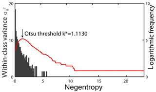
where ${{\mathit{\sigma }}_B}^{\mathrm{2}}$ is the within-class variance of negentropy. Then, by finding the k^* value searching for k when ${{\mathit{\sigma }}_B}^{\mathrm{2}}$ becomes the maximum,

$$\begin{array}{}\text{(16)}& k^{*}=\arg \underset{k}{max}{{\mathit{\sigma }}_B}^{\mathrm{2}}\left(k\right),\end{array}$$

where the optimal value k^* here separates the background set and anomaly set.

In this test, our initial assumption is that the sliding window is composed of a Gaussian signal of non-seismic-related activities. When our test negentropy exceeds the critical value k^*, this initial hypothesis is not valid, and the alternative is true, indicating the presence of a negentropy anomaly within the window.

4 Results

According to the empirical hypothesis that geophysical signals deviate from the Gaussian distribution when they record abnormal activities, and based on the results of previous studies, we perform the following investigation.

4.1 Extracting negentropy anomalies

As the negentropy is calculated using a 2 h sliding window, we assume that it reaches the maximum values when the time window contains anomalies from seismic-related activities. The negentropy during the study period is shown in Fig. 4.

Figure 4 Negentropy at Guza from 1 January 2007 to 30 June 2009. The red dotted horizontal line is the optimal threshold k^* calculated by Otsu method.

The within-class variance ${{\mathit{\sigma }}_B}^{\mathrm{2}}$ and negentropy value distribution are compared in Fig. 5. According to Eqs. (11) to (14), when $k^{*}=\mathrm{1.1130}$, ${{\mathit{\sigma }}_B}^{\mathrm{2}}$ reaches its maximum. Therefore, the negentropy was separated by k^* into the quasi-Gaussian background and non-Gaussian anomalies from 2007 to 2009. The Otsu threshold k^* here is consistent with the accuracy of the negentropy and the strain data. The YRY-4 borehole strainmeter has a measurement accuracy of 10⁻⁹; however, we usually cut off four digits after the decimal point in practical calculations.

Figure 5 Within-class variance ${{\mathit{\sigma }}_B}^{\mathrm{2}}$ in the negentropy (red line) and negentropy histogram.

In the skewness–kurtosis domain, the statistical relationship of the borehole areal strain is consistent with parabolic behaviour as described in Eq. (10) (Fig. 6a), verifying that the turbulent system of borehole strain is significantly non-Gaussian. Besides this, the extracted negentropy anomalies are clustered strongly on the left side of the parabola, which exhibits similar characteristics different from the normal Gaussian distribution. Here, there are four points on the right side; one occurred in early 2007, and the others occurred after the earthquake. Therefore, we will not discuss them in the following.

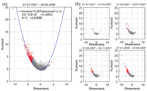
Figure 6 Negentropy distributions in the skewness–kurtosis domain in (a) 1 January 2007 to 30 June 2009, and (b) four shorter periods before the earthquake. Red denotes the negentropy being greater than k^*, and grey indicates the negentropy being less than k^*. The blue curve is the quadratic fit with 95 % confidence.

In addition, as shown in Fig. 6b, at times far from the earthquake, the negentropy distribution is basically Gaussian in the skewness–kurtosis domain. However, at times closer to the earthquake, the relatively stable state was broken due to the non-Gaussian mechanism, with more negentropy anomalies appearing on the left side of the parabola, while in 2008, almost all of the negentropy present was skewed to the left.

The phenomena prompt us to study its possible correspondence with the seismogenic process.

4.2 Negentropy anomaly frequency accumulation

The transition of negentropy anomalies in the skewness–kurtosis domain is quantified as the change of the anomaly frequency per unit time through a logarithmic-linear model. Logarithmic-linear models of interest are often used to estimate the expected frequency of the response variable at the original scale for a new set of covariate values, such as the Gutenberg–Richer law, in which a linear relationship exists between the logarithm of the cumulative number of seismic events of magnitude M or greater versus the magnitude M (Gutenberg and Richter, 1954).

The logarithmic-linear regression model is proposed as

$$\begin{array}{}\text{(17)}& \log N={\mathit{\beta }}_{\mathrm{1}}\times k_J+{\mathit{\beta }}_{\mathrm{0}}+\mathit{\epsilon },\end{array}$$

where k_J takes different threshold values according to the J(x) values, N is the number of occurrences in which J is greater than or equal to the threshold k_J, β₁ and β₀ are the regression coefficients, where a lower slope β₁ indicates that there are more higher J values, implying that there are more anomalies at that moment, and ε is the random error that represents the model uncertainty.

We use the logarithmic-linear model to solve the relationship between the negentropy anomaly frequency and different thresholds each day using the ordinary least-squares (OLS) method. Afterwards, an optimal threshold k^*, calculated by the Otsu method, is chosen for all models, where

$$\begin{array}{}\text{(18)}& N_J\left(t\right)=\exp \left({\mathit{\beta }}_{\mathrm{1}}\left(t\right)\times k^{*}+{\mathit{\beta }}_{\mathrm{0}}\left(t\right)+\mathit{\epsilon }\left(t\right)\right),\end{array}$$

and the N_J(t) under the threshold k^* is shown in Fig. 7. The model theoretically solves the problem of selecting the length of the time window. In addition, the estimated N_J(t) is considered to be the expected frequency of anomalies.

The goodness of fit for each logarithmic-linear model was evaluated using analysis of

$$\begin{array}{}\text{(19)}& R^{\mathrm{2}}=\mathrm{1}-\sum _{i=\mathrm{1}}^n{\left(N_i-\widehat{N_i}\right)}^{\mathrm{2}}/\sum _{i=\mathrm{1}}^n{\left(N_i-\stackrel{\mathrm{‾}}{N_i}\right)}^{\mathrm{2}},\end{array}$$

and the root-mean-squared error (RMSE):

$$\begin{array}{}\text{(20)}& \mathrm{RMSE}=\sqrt{\sum _{i=\mathrm{1}}^n{\left(N_i-\widehat{N_i}\right)}^{\mathrm{2}}/n}.\end{array}$$

The R² and RMSE values in the study period (912 d) show that the logarithmic-linear relationship can explain the relationship between the negentropy anomaly frequency and different thresholds. The mean of R² is 0.9695, which is close to 1, and the variance of R² is 0.0435. The mean and variance of the RMSE are also small (0.1098 and 0.1301, respectively).

Figure 7 Estimated expected frequency N_J under the optimal threshold k^*.

We calculate the negentropy cumulative frequency of the study period, as shown in Fig. 8. There is not only a long-term analysis of the whole period, but also a short-term analysis of the pre-earthquake process. In general, accumulated value of a typical random process usually has a linear increase. In particular, in case of critical phenomena, we would expect more frequent anomalies when they approach the critical point and less frequent anomalies after Santis et al. (2017).

For the entire earthquake process, a 2-month sliding window is selected for accumulation. In Fig. 8a, after July 2007, the negentropy anomalies gradually accumulated. Qiu (2009) and Chi (2014) also observed anomalies of this period at the Guza station, and they speculated that abnormal strain may reflect small-scale rock formation rupture before the earthquake. In particular, we find more frequent negentropy anomalies in 2008 as the earthquake approaches and less frequent anomalies after the earthquake; thus a sigmoid function is used to fit the acceleration before the earthquake and to fit the deceleration after the earthquake. The sigmoid function is expressed as

$$\begin{array}{}\text{(21)}& y=A\mathrm{2}+{\displaystyle \frac{\left(A\mathrm{1}-A\mathrm{2}\right)}{\left(\mathrm{1}+e^{\frac{x-x_{\mathrm{0}}}{\mathrm{d}x}}\right)}},\end{array}$$

where A1, A2, x0 and dx are the inflection point. The sigmoid function is a power-law temporal behaviour, with an upper concavity, and a subsequent power-law behaviour after the inflection point, with an opposite concavity. The inflection point in this function is a reasonable estimation of the time of the significant change in the critical dynamical system (Santis et al., 2017). Also, the value of x0 (8.3337) obtained in the fitting almost coincides with the day of the Wenchuan earthquake. The actual time of the earthquake is the 8.3871th bimonth from January 2007 after conversion.

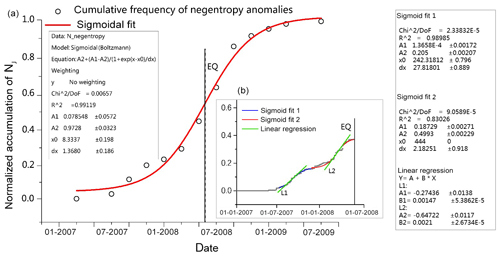
Figure 8 (a) Results of the long-term negentropy anomaly frequency for the Wenchuan earthquake at Guza station from 1 January 2007 to 30 June 2009. Each circle represents an anomaly negentropy for 2 months. The cumulative frequency of negentropy anomaly is represented. The earthquake day is represented as a black vertical dashed line. The red line is a sigmoid fit that underlines an inflection point (vertical solid line) that is close to the occurrence of the earthquake. (b) Results of the short-term negentropy anomaly frequency prior to the earthquake. Every grey point is an anomaly for 1 d, and the blue and red lines are two segment sigmoid fit results. Two green lines represent the liner regression for the two phases; the first phase slope is 0.00147, and the second one is 0.0021.

When we narrowed the accumulated window to 1 d, we observed two negentropy anomalies before the earthquake, as shown in Fig. 8b. The first anomaly frequency increase occurred from August to October 2007. In March 2008, there was a second phase of anomaly increase, and the cumulative frequency then slowly increased to a plateau period near the time of the earthquake. This, probably due to the stress, is in a deadlocked phase. This is because before the Wenchuan earthquake, the elastic deformation of the crust reaches its limit and the deformation is resisted in the hypocentral region, which is measured by GPS data (Jiang et al., 2009).

These two phases prior to the earthquake are also approximated with sigmoid functions. In order to further compare the anomalies of the two phases, we use linear regression to fit the central part of the two sigmoid curves. We find that the second acceleration is greater than the first acceleration.

Fault zones contain relatively weak and relatively strong parts. The former is the area where strain release begins, while the latter is the stress-locking part and the beginning of rapid instability (Noda et al., 2013). Ma and Guo (2014) proposed that there is a sub-instability stage of fault deformation before earthquakes, which is manifested by two instability activities. The former is related to the release of weak parts, and the latter is related to the rapid release of strong parts during strong earthquakes. They thought that acceleration of the strain release in fault zone is a sign of entering the inevitable earthquake stage. Thus, we speculate that the two accelerations of the cumulative negentropy anomaly in Fig. 8b may be related to the strong earthquake.

5 Comparison discussion

5.1 Comparison of random time periods.

We randomly selected the strain data for 200 d before and after 20 March 2011 and 24 March 2014 at the Guza station. The selected data for the two periods are required to be in the absence of strong earthquakes and have higher quality. We performed negentropy analysis on these two observations and compared them with the results of negentropy analysis associated with the Wenchuan earthquake, as shown in Fig. 9.

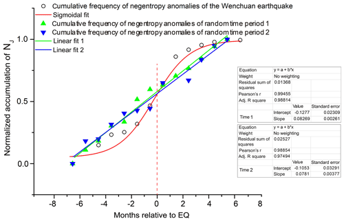
Figure 9 The comparative analysis of cumulative frequency of negentropy anomalies between earthquake period and random time periods. The zero point of green dots is 20 March 2011, and the zero point of blue dots is 24 March 2014.

As we can see in Fig. 9, the cumulative frequency of negentropy anomalies of random periods has a linear increase. However, in the Wenchuan-earthquake periods, as the earthquake approaches, the cumulative frequency of negentropy anomalies increases rapidly and recovered to a slow growth after the earthquake.

5.2 Comparison of different stations

We selected the Xiaomiao station and Renhe station to find out if their observations received strain changes. Their locations are shown in Fig. 1. Compared with the Guza station, we did the negentropy analysis of these two stations, as shown in Fig. 10.

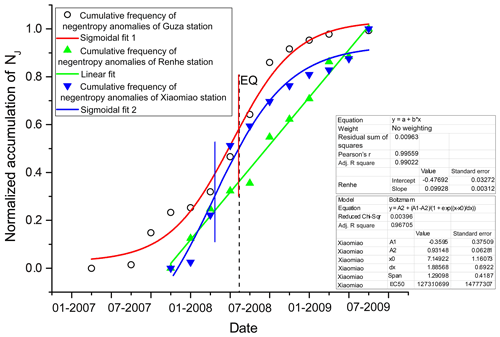
Figure 10 Cumulative frequency of negentropy anomalies of Xiaomiao station and Renhe station from 16 September 2007 to 30 June 2009. The negentropy analysis of Guza station is from 1 January 2007 to 30 June 2009 because of the different installation time of the instruments. The red vertical line is the inflection point of the fitting curve of Guza station. The blue vertical line is the inflection point of the fitting curve of Xiaomiao station. The black dotted line is the earthquake day.

As we can see in the Fig. 10, the cumulative frequency of negentropy anomalies of the Xiaomiao station is also well fitted by the sigmoid function. The accumulation curve grows rapidly before the earthquake and is concave downward after the earthquake, which is similar to the Guza station, although the inflection point of the Xiaomiao station precedes the earthquake moment by about 2 months. However, since the curve is approximately linear before and after the inflection point, we consider that the inflection point value is reasonable in the range from January to June 2008. Cumulative anomalies of the Renhe station are basically linear, indicating that the Renhe station may not detect pre-earthquake anomalies.

The Renhe station is far from the end of the Wenchuan-earthquake fault, so it is reasonable that no abnormal changes are observed. However, the Xiaomiao station is located between the Guza station and Renhe station, and the fitting result shows that there is a similar trend to the Guza station, with a weaker curvature. So, for the nearest station to the epicentre, the Guza station may be able to record more pre-earthquake anomalies.

Furthermore, Qiu et al. (2012) found that the anomalies at the Ningshan station were similar to the anomalies at the Guza station. These two stations have observed similar Wenchuan-earthquake precursor anomalies, which may not be accidental, since the Ningshan station is actually located at the northeastern end of the Longmenshan Fault zone. This location corresponds with the southwestern end of the fault, where the Guza station is located.

5.3 Exclusion of meteorological factors.

The strain signals are sensitive to a few meteorological factors; therefore, we display the pressure variations, temperature variations recorded at the Guza station and the daily rainfall measured by Tropical Rainfall Measuring Mission (TRMM) satellite, which can be downloaded through NASA Giovanni-4 for the same period and the same area (http://giovanni.gsfc.nasa.gov/giovanni/, last access: 18 October 2019) in Fig. 11. There are clearly annual variations in the strain, air pressure, temperature and rainfall data. The air pressure and temperature have been steadily fluctuating within a certain range, and the rainfall has also proved to be more in summer and less in winter.

Then we calculated the differential data of the strain for negentropy analysis. We also make differential calculations for all three influencing factors, as shown in Fig. 12.

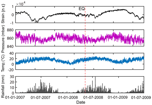
Figure 11 Borehole stain, air pressure, temperature and rainfall variations during study period at Guza station.

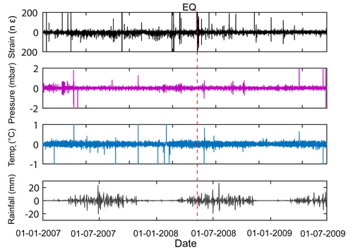
Figure 12 Differential borehole stain, air pressure, temperature and rainfall variations during study period at Guza station.

We observed that the air pressure, temperature and rainfall did not change abnormally during the period when the extracted anomalies increase whether we do differential calculation or not. Therefore, we consider that the abnormal variations on the processed strain signals are not caused by these factors.

6 Conclusions

In our work, the extracted negentropy anomalies of borehole strain associated with the Wenchuan earthquake are analysed. The cumulative frequency of negentropy anomalies are studied in both the long and short term. In the Comparison discussion section, we compare the cumulative anomalies of different time periods and different stations with those at the Guza station during the study period and preliminarily exclude meteorological factors. We suspect that the negentropy anomalies at the Guza station may have recorded abnormal changes related to the Wenchuan earthquake.

Since the tectonic dynamics of earthquakes during seismogenic and seismic processes are very complex, the mechanism of such abnormal changes undoubtedly needs to be discussed. In particular, borehole strain signals are sensitive to external influence. Besides this, because of the different characteristics and accuracy of different types of observations, a joint analysis has not been carried out yet. Further research is needed to decipher a potential precursory phase. However, we may be able to ensure that the negentropy analysis has great potential in the study of earthquake precursors.