the Creative Commons Attribution 4.0 License.
the Creative Commons Attribution 4.0 License.
 | 17 Sep 2019
Revising the stochastic iterative ensemble smoother
Patrick Nima Raanes
Andreas Størksen Stordal
Geir Evensen
Ensemble randomized maximum likelihood (EnRML) is an iterative (stochastic) ensemble smoother, used for large and nonlinear inverse problems, such as history matching and data assimilation. Its current formulation is overly complicated and has issues with computational costs, noise, and covariance localization, even causing some practitioners to omit crucial prior information. This paper resolves these difficulties and streamlines the algorithm without changing its output. These simplifications are achieved through the careful treatment of the linearizations and subspaces. For example, it is shown (a) how ensemble linearizations relate to average sensitivity and (b) that the ensemble does not lose rank during updates. The paper also draws significantly on the theory of the (deterministic) iterative ensemble Kalman smoother (IEnKS). Comparative benchmarks are obtained with the Lorenz 96 model with these two smoothers and the ensemble smoother using multiple data assimilation (ES-MDA).
- Article
(1309 KB) - Full-text XML
- BibTeX
- EndNote


Ensemble (Kalman) smoothers are approximate methods used for data assimilation (state estimation in geoscience), history matching (parameter estimation for petroleum reservoirs), and other inverse problems constrained by partial differential equations. Iterative forms of these smoothers, derived from optimization perspectives, have proven useful in improving the estimation accuracy when the forward operator is nonlinear. Ensemble randomized maximum likelihood (EnRML) is one such method.
This paper rectifies several conceptual and computational complications with EnRML, detailed in Sect. 1.1. As emphasized in Sect. 1.2, these improvements are largely inspired by the theory of the iterative ensemble Kalman smoother (IEnKS). Readers unfamiliar with EnRML may jump to the beginning of the derivation, starting in Sect. 2, which defines the inverse problem and the idea of the randomized maximum likelihood method. Section 3 derives the new formulation of EnRML, which is summarized by Algorithm 1 of Sect. 3.7. Section 4 shows benchmark experiments obtained with various iterative ensemble smoothers. Appendix A provides proofs of some of the mathematical results used in the text.
1.1 Ensemble randomized maximum likelihood (EnRML): obstacles
The Gauss–Newton variant of EnRML was given by Gu and Oliver (2007) and Chen and Oliver (2012), with an important precursor from Reynolds et al. (2006). This version explicitly requires the ensemble-estimated “model sensitivity” matrix, herein denoted . As detailed in Sect. 3, this is problematic because is noisy and requires the computation of the pseudo-inverse of the “anomalies”, , for each iteration, i.
A Levenberg–Marquardt variant was proposed in the landmark paper of Chen and Oliver (2013b). Its main originality is a partial resolution to the above issue by modifying the Hessian matrix (beyond the standard trust-region step regularization): the prior ensemble covariance matrix is replaced by the posterior covariance (of iteration i): . Now the Kalman gain form of the likelihood increment is “vastly simplified” because the linearization only appears in the product , which does not require . For the prior increment, on the other hand, the modification breaks its Kalman gain form. Meanwhile, the precision matrix form, i.e. their Eq. (10), is already invalid because it requires the inverse of . Still, in their Eq. (15), the prior increment is formulated with an inversion in ensemble space and also unburdened of the explicit computation of . Intermediate explanations are lacking but could be construed to involve approximate inversions. Another issue is that the pseudo-inverse of is now required (via X), and covariance localization is further complicated.
An approximate version was therefore also proposed in which the prior mismatch term is omitted from the update formula altogether. This is not principled and severely aggravates the chance of overfitting and poor prediction skill. Therefore, unless the prior mismatch term is relatively insignificant, overfitting must be prevented by limiting the number of steps or by clever stopping criteria. Nevertheless, this version has received significant attention in history matching.
This paper revises EnRML; without any of the above tricks, we formulate the algorithm such that there is no explicit computation of and show how the product may be computed without any pseudo-inversions of the matrix of anomalies. Consequently, the algorithm is simplified, computationally and conceptually, and there is no longer any reason to omit the prior increment. Moreover, the Levenberg–Marquardt variant is a trivial modification of the Gauss–Newton variant. The above is achieved by improvements to the derivation, notably by (a) improving the understanding of the sensitivity (i.e. linearizations) involved, (b) explicitly and rigorously treating issues of rank deficiency and subspaces, and (c) avoiding premature insertion of singular value decompositions (SVDs).
1.2 Iterative ensemble Kalman smoother (IEnKS)
The contributions of this paper (listed by the previous paragraph) are original but draw heavily on the theory of the IEnKS of Sakov et al. (2012) and Bocquet and Sakov (2012, 2014). Relevant precursors include Zupanski (2005) as well as the iterative, extended Kalman filter (e.g. Jazwinski, 1970).
It is informally known that EnRML can be seen as a stochastic flavour of the IEnKS (Sakov et al., 2012). Indeed, while the IEnKS update takes the form of a deterministic, “square-root” transformation, based on a single objective function, EnRML uses stochastic “perturbed observations” associated with an ensemble of randomized objective functions.
Another notable difference is that the IEnKS was developed in the atmospheric literature, while EnRML was developed in the literature on subsurface flow. Thus, typically, the IEnKS is applied to (sequential) state estimation problems such as filtering for chaotic dynamical systems, while EnRML is applied to (batch) parameter estimation problems, such as nonlinear inversion for physical constants and boundary conditions. For these problems, EnRML is sometimes referred to as the iterative ensemble smoother (IES). As shown by Gu and Oliver (2007), however, EnRML is easily reformulated for the sequential problem, and, vice versa, the IEnKS may be formulated for the batch problem.
The improvements to the EnRML algorithm herein render it very similar to the IEnKS also in computational cost. It thus fully establishes that EnRML is the stochastic “counterpart” to the IEnKS. In spite of the similarities, the theoretical insights and comparative experiments of this paper should make it interesting also for readers already familiar with the IEnKS.
Randomized maximum likelihood (RML; Kitanidis, 1995; Oliver, 1996; Oliver et al., 2008) is an approximate solution approach to a class of inverse problems. The form of RML described here is a simplification, common for large inverse problems, without the use of a correction step (such as that of Metropolis–Hastings). This restricts the class of problems for which it is unbiased but makes it more tractable (Oliver, 2017). Similar methods were proposed and studied by Bardsley et al. (2014), Liu et al. (2017), and Morzfeld et al. (2018).
2.1 The inverse problem
Consider the problem of estimating the unknown, high-dimensional state (or parameter) vector x∈ℝM given the observation y∈ℝP. It is assumed that the (generic and typically nonlinear) forward observation process may be approximated by a computational model, ℳ, so that
where the error, δ, is random and gives rise to a likelihood, p(y|x).
In the Bayesian paradigm, prior information is quantified as a probability density function (PDF) called the prior, denoted p(x), and the truth, x, is considered to be a draw thereof. The inverse problem then consists of computing and representing the posterior which, in principle, is given by pointwise multiplication:
quantifying the updated estimation of x. Due to the noted high dimensionality and nonlinearity, this can be challenging, necessitating approximate solutions.
The prior is assumed Gaussian (normal), with mean μx and covariance Cx, i.e.
For now, the prior covariance matrix, , is assumed invertible such that the corresponding norm, , is defined. Note that vectors are taken to have column orientation and that xT denotes the transpose.
The observation error, δ, is assumed drawn from
whose covariance, , will always be assumed invertible. Then, assuming that δ and x are independent and recalling Eq. (1),
2.2 Randomize, then optimize
The Monte Carlo approach offers a convenient representation of distributions as samples. Here, the prior is represented by the “prior ensemble”, , whose members (sample points) are assumed independently drawn from it. RML is an efficient method to approximately “condition” (i.e. implement Eq. 2 on) the prior ensemble, using optimization. Firstly, an ensemble of perturbed observations, , is generated as , where δn is independently drawn according to Eq. (4).
Then, the nth “randomized log posterior”, Jx,n, is defined by Bayes' rule (Eq. 2), except with the prior mean and the observation being replaced by the nth members of the prior and observation ensembles:
The two terms are referred to as the model mismatch (log prior) and data mismatch (log likelihood), respectively.
Finally, these log posteriors are minimized. Using the Gauss–Newton iterative scheme (for example) requires (Eq. 7a) its gradient and (Eq. 7b) its Hessian approximated by first-order model expansions, both evaluated at the current iterate, labelled xn,i for each member n and iteration i. To simplify the notation, define . Objects evaluated at x× are similarly denoted; for instance, denotes the Jacobian matrix of ℳ evaluated at x×, and
Application of the Gauss–Newton scheme yields
where the prior (or model) and likelihood (or data) increments are respectively given by
which can be called the “precision matrix” form.
Alternatively, by corollaries of the well-known Woodbury matrix identity, the increments can be written in the “Kalman gain” form:
where is the identity matrix, and is the gain matrix,
with
As the subscript suggests, Cy may be identified (in the linear case) as the prior covariance of the observation, y, of Eq. (1); it is also the covariance of the innovation, y−ℳ(μx). Note that if P≪M, then the inversion of for the Kalman gain form, Eq. (10a) and (10b), is significantly cheaper than the inversion of for the precision matrix form, Eq. (9a) and (9b).
EnRML is an approximation of RML in which the ensemble is used in its own update by estimating Cx and M×. This section derives EnRML and gradually introduces the new improvements.
Computationally, compared to RML, EnRML offers the simultaneous benefits of working with low-rank representations of covariances and not requiring a tangent-linear (or adjoint) model. Both advantages will be further exploited in the new formulation of EnRML.
Concerning their sampling properties, a few points can be made. Firstly (due to the ensemble covariance), EnRML is biased for finite N, even for a linear-Gaussian problem for which RML will sample the posterior correctly. This bias arises for the same reasons as in the ensemble Kalman filter (EnKF; van Leeuwen, 1999; Sacher and Bartello, 2008). Secondly (due to the ensemble linearization), EnRML effectively smoothes the likelihood. It is therefore less prone to getting trapped in local maxima of the posterior (Chen and Oliver, 2012). Sakov et al. (2018) explain this by drawing an analogy to the secant method, as compared to the Newton method. Hence, it may reasonably be expected that EnRML yields constructive results if the probability mass of the exact posterior is concentrated around its global maximum. Although this regularity condition is rather vague, it would require that the model be “not too nonlinear” in this neighbourhood. Conversely, EnRML is wholly inept at reflecting multimodality introduced through the likelihood, so RML may be better suited when local modes feature prominently, as is quite common in problems of subsurface flow (Oliver and Chen, 2011). However, while RML has the ability to sample multiple modes, it is difficult to predict the extent to which their relative proportions will be accurate (without the costly use of a correction step such as Metropolis–Hastings). Further comparison of the sampling properties of RML and EnRML was done by Evensen (2018).
3.1 Ensemble preliminaries
For convenience, define the concatenations:
which are known as the “ensemble matrix” and the “perturbation matrix”, respectively.
Projections sometimes appear through the use of linear regression. We therefore recall (Trefethen and Bau, 1997) that a (square) matrix Π is an orthogonal projector if
For any matrix A, let ΠA denote the projector whose image is the column space of A, implying that
Equivalently, , where , is called the complementary projector. The (Moore–Penrose) pseudo-inverse, A+, may be used to express the projector
Here, the second equality follows from the first by Eq. (15) and . The formulae simplify further in terms of the SVD of A.
Now, denote 1∈ℝN the (column) vector of ones. The matrix of anomalies, , is defined and computed by subtracting the ensemble mean, , from each column of E. It should be appreciated that this amounts to the projection
where , with .
Definition 1: the ensemble subspace. The flat (i.e. affine subspace) given by .
Similarly to Sect. 2, the iteration index (i>0) subscripting on E, X, and other objects is used to indicate that they are conditional (i.e. posterior). The iterations are initialized with the prior ensemble: .
3.2 The constituent estimates
The ensemble estimates of Cx and M× are the building blocks of the EnRML algorithm. The canonical estimators are used, namely the sample covariance (Eq. 19a) and the least-squares linear-regression coefficients (Eq. 19b). They are denoted with the overhead bar:
The anomalies at iteration i are again given by , usually computed by subtraction of . The matrix ℳ(Ei) is defined by the column-wise application of ℳ to the ensemble members. Conventionally, ℳ(Ei) would also be centred in Eq. (19b), i.e. multiplied on the right by . However, this operation (and notational burden) can be neglected because , which follows from (valid for any matrix A and projector Π, as shown by Maciejewski and Klein, 1985).
Note that the linearization (previously M×, now ) no longer depends on the ensemble index, n. Indeed, it has been called “average sensitivity” since the work of Zafari and Reynolds (2005), Reynolds et al. (2006), and Gu and Oliver (2007). However, this intuition has not been rigorously justified.1 This is accomplished by the following theorem.
Suppose the ensemble is drawn from a Gaussian. Then
with “almost sure” convergence, and expectation (𝔼) in x, which has the same distribution as the ensemble members. Regularity conditions and proof may be found in Appendix A.
A corollary of Theorem 1 is that , justifying the “average sensitivity, derivative, or gradient” description. The theorem applies for the ensemble of any Gaussian, and hence also holds for . On the other hand, the generality of Theorem 1 is restricted by the Gaussianity assumption. Thus, for generality and precision, should simply be labelled the “least-squares (linear) fit” of ℳ, based on Ei.
Note that the computation (Eq. 19b) of seemingly requires calculating a new pseudo-inverse, , at each iteration, i; this is addressed in Sect. 3.6.
The prior covariance estimate (previously Cx, now ) is not assumed invertible, in contrast to Sect. 2. It is then not possible to employ the precision matrix forms, Eq. (9a) and (9b), because is not defined. Using the in its stead is flawed and damaging because it is zero in the directions orthogonal to the ensemble subspace, so its use would imply that the prior is assumed infinitely uncertain (i.e. flat) as opposed to infinitely certain (like a delta function) in those directions. Instead, one should employ ensemble subspace formulae or, equivalently (as shown in the following, using corollaries of the Woodbury identity), the Kalman gain form.
3.3 Estimating the Kalman gain
The ensemble estimates, Eq. (19a) and (19b), are now substituted into the Kalman gain form of the update (Eq. 10a and 10b to Eq. 12). The ensemble estimate of the gain matrix, denoted , thus becomes
where has been defined as the prior (i.e. unconditioned) anomalies under the action of the ith iterate linearization:
A Woodbury corollary can be used to express as
with
The reason for labelling this matrix with the subscript w is revealed later. For now, note that, in the common case of N≪P, the inversion in Eq. (24) is significantly cheaper than the inversion in Eq. (21). Another computational benefit is that is non-dimensional, improving the conditioning of the optimization problem (Lorenc, 1997).
In conclusion, the likelihood increment (Eq. 10b) is now estimated as
This is efficient because does not explicitly appear in (neither in Eq. 21 nor Eq. 23) even though it is implicitly present through Yi (Eq. 22), where it multiplies X. This absence (a) is reassuring, as the product Yi constitutes a less noisy estimate than just alone (Chen and Oliver, 2012; Emerick and Reynolds, 2013b, their Figs. 2 and 27, respectively), (b) constitutes a computational advantage, as will be shown in Sect. 3.6, and (c) enables leaving the type of linearization made for ℳ unspecified, as is usually the case in EnKF literature.
3.4 Estimating the prior increment
In contrast to the likelihood increment (Eq. 10b), the Kalman gain form of the prior increment (Eq. 10a) explicitly contains the sensitivity matrix, M×. This issue was resolved by Bocquet and Sakov (2012) in their refinement of Sakov et al. (2012) by employing the change of variables:
where w∈ℝN is called the ensemble “controls” (Bannister, 2016), also known as the ensemble “weights” (Ott et al., 2004) or “coefficients” (Bocquet and Sakov, 2013).
Denote w×, an ensemble coefficient vector, such that , and note that x(en)=xn, where en is the nth column of the identity matrix. Thus, , and the prior increment (Eq. 10a) with the ensemble estimates becomes
where there is no explicit , which only appears implicitly through , as defined in Eq. (22) Alternatively, applying the subspace formula (Eq. 23) and using yields
3.5 Justifying the change of variables
Lemma 1 (closure). Suppose Ei is generated by EnRML. Then, each member (column) of Ei is in the (prior) ensemble subspace. Moreover, col(Xi)⊆col(X).
Lemma 1 may be proven by noting that X is the leftmost factor in and using induction on Eqs. (10a) and (10b). Alternatively, it can be deduced (Raanes et al., 2019) as a consequence of the implicit assumption on the prior that . A stronger result, namely col(Xi)=col(X), is conjectured in Appendix A, but Lemma 1 is sufficient for the present purposes: it implies that exists such that for any ensemble member and any iteration. Thus, the lemma justifies the change of variables (Eq. 26).
Moreover, using the ensemble coefficient vector (w) is theoretically advantageous, as it inherently embodies the restriction to the ensemble subspace. A practical advantage is that w is relatively low-dimensional compared to x, which lowers storage and accessing expenses.
3.6 Simplifying the regression
Recall the definition of Eq. (22): . Avoiding the explicit computation of used in this product between the iteration-i estimate and the initial (prior) X was the motivation behind the modification by Chen and Oliver (2013b). Here, instead, by simplifying the expression of the regression, it is shown how to compute Yi without first computing .
3.6.1 The transform matrix
Inserting the regression (19b) into the definition (22),
where has been defined, apparently requiring the pseudo-inversion of Xi for each i. But, as shown in Appendix A2,
which only requires the one-time pseudo-inversion of the prior anomalies, X. Then, since the pseudo-inversion of for Yi (29) is a relatively small calculation, this saves computational time.
The symbol T has been chosen in reference to deterministic, square-root EnKFs. Indeed, multiplying Eq. (30) on the left by X and recalling Eq. (17) and Lemma 1 produces Xi=XTi. Therefore, the “transform matrix”, Ti, describes the conditioning of the anomalies (and covariance).
Conversely, Eq. (29) can be seen as the “de-conditioning” of the posterior observation anomalies. This interpretation of Yi should be contrasted to its definition (22), which presents it as the prior state anomalies “propagated” by the linearization of iteration i. The two approaches are known to be “mainly equivalent” in the deterministic case (Sakov et al., 2012). To our knowledge, however, it has not been exploited for EnRML before now, possibly because the proofs (Appendix A2) are a little more complicated in this stochastic case.
3.6.2 From the ensemble coefficients
The ensemble matrix of iteration i can be written as follows:
where the columns of are the ensemble coefficient vectors (Eq. 26). Multiplying Eq. (31) on the right by to get the anomalies produces
This seems to indicate that is the transform matrix, Ti, discussed in the previous subsection. However, they are not fully equal: inserting Xi from Eq. (32) into Eq. (30) yields
showing that they are distinguished by : the projection onto the row space of X.
Appendix A3 shows that, in most conditions, this pesky projection matrix vanishes when Ti is used in Eq. (29):
In other words, the projection can be omitted unless ℳ is nonlinear and the ensemble is larger than the unknown state's dimensionality.
A well-known result of Reynolds et al. (2006) is that the first step of the EnRML algorithm (with W0=IN) is equivalent to the EnKF. However, this is only strictly true if there is no appearance of in EnRML. The following section explains why EnRML should indeed always be defined without this projection.
3.6.3 Linearization chaining
Consider applying the change of variables 26 to w at the very beginning of the derivation of EnRML. Since X1=0, there is a redundant degree of freedom in w, meaning that there is a choice to be made in deriving its density from the original one, given by Jx,n(x) in Eq. (6). The simplest choice (Bocquet et al., 2015) results in the log posterior:
Application of the Gauss–Newton scheme with the gradients and Hessian matrix of Jw,n, followed by a reversion to x, produces the same EnRML algorithm as above.
The derivation summarized in the previous paragraph is arguably simpler than that of the last few pages. Notably, (a) it does not require the Woodbury identity to derive the subspace formulae, (b) there is never an explicit to deal with, and (c) the statistical linearization of least-squares regression from Wi to ℳ(Ei) directly yields Eq. (34), except that there are no preconditions.
While the case of a large ensemble () is not typical in geoscience, the fact that this derivation does not produce a projection matrix (which requires a pseudo-inversion) under any conditions begs the following questions. Why are they different? Which version is better?
The answers lie in understanding the linearization of the map and noting that, similarly to analytical (infinitesimal) derivatives, the chain rule applies for least-squares regression. In effect, the product , which implicitly contains the projection matrix , can be seen as an application of the chain rule for the composite function ℳ(x(w)). By contrast, Eq. (34) – but without the precondition – is obtained by direct regression of the composite function. Typically, the two versions yield identical results (i.e. the chain rule). However, since the intermediate space, col(X), is of lower dimensions than the initial domain (), composite linearization results in a loss of information, manifested by the projection matrix. Therefore, the definition is henceforth preferred to .
Numerical experiments, as in Sect. 4 but not shown, indicate no statistically significant advantage for either version. This corroborates similar findings by Sakov et al. (2012) for the deterministic flavour. Nevertheless, there is a practical advantage: avoiding the computation of .
3.6.4 Inverting the transform
In square-root ensemble filters, the transform matrix should have 1 as an eigenvector (Sakov and Oke, 2008; Livings et al., 2008). By construction, this also holds true for , with eigenvalue 0. Now, consider adding 0=XΠ1 to Eq. (32), yielding another valid transformation:
The matrix Ωi, in contrast to and Ti, has eigenvalue 1 for 1 and is thus invertible. This is used to prove Eq. (34) in Appendix A3, where Yi is expressed in terms of .
Numerically, the use of Ωi in the computation (34) of Yi was found to yield stable convergence of the new EnRML algorithm in the trivial example of ℳ(x)=αx. By contrast, the use of exhibited geometrically growing (in i) errors when α>1. Other formulae for the inversion are derived in Appendix A4. The one found to be the most stable is ; it is therefore preferred in Algorithm 1.
Irrespective of the inverse transform formula used, it is important to retain all non-zero singular values. This absence of a truncation threshold is a tuning simplification compared with the old EnRML algorithm, where X and/or Xi was scaled, decomposed, and truncated. If, by extreme chance or poor numerical subroutines, the matrix Wi is not invertible (this never occurred in any of the experiments except by our manual intervention; see the conjecture in Appendix A), its pseudo-inversion should be used; however, this must also be accounted for in the prior increment by multiplying the formula on line 8 on the left by the projection onto Wi.
3.7 Algorithm
To summarize, Algorithm 1 provides pseudo-code for the new EnRML formulation. The increments (Eq. 25) and (Eq. 28) can be recognized by multiplying line 10 on the left by X. For aesthetics, the sign of the gradients has been reversed. Note that there is no need for an explicit iteration index. Nor is there an ensemble index, n, since all N columns are stacked into the matrix W. However, in case M is large, Y may be computed column by column to avoid storing E.
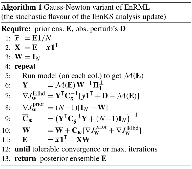
Line 6 is typically computed by solving for Y′ and then subtracting its column mean. Alternative formulae are discussed in Sect. 3.6.4. Line 9 may be computed using a reduced (or even truncated) SVD of , which is relatively fast for N both larger and smaller than P. Alternatively, the Kalman gain forms could be used.
The Levenberg–Marquardt variant is obtained by adding the trust-region parameter λ>0 to (N−1) in the Hessian matrix (line 9), which impacts both the step length and direction.
Localization may be implemented by local analysis (Hunt et al., 2007; Sakov and Bertino, 2011; Bocquet, 2016; Chen and Oliver, 2017). Here, tapering is applied by replacing the local-domain (implicit on lines 7 and 9) by , with ∘ being the Schur product and ρ a square matrix containing the (square-root) tapering coefficients, . If the number of local domains used is large so that the number of W matrices used becomes large, then it may be more efficient to revert to the original state variables and explicitly compute the sensitivities using the local parts of ℳ(Ei) and Xi.
Inflation and model error parameterizations are not included in the algorithm but may be applied outside of it. We refer to Sakov et al. (2018) and Evensen (2019) for model error treatment with iterative methods.
The new EnRML algorithm produces results that are identical to the old formulation, at least up to round-off and truncation errors, and for . Therefore, since there are already a large number of studies of EnRML with reservoir cases (e.g. Chen and Oliver, 2013a; Emerick and Reynolds, 2013b), adding to this does not seem necessary.
However, there do not appear to be any studies of EnRML with the Lorenz 96 system (Lorenz, 1996) in a data assimilation setting. The advantages of this case are numerous: (a) the model is a surrogate of weather dynamics and as such holds relevance in geoscience, (b) the problem is (exhaustively) sampled from the system's invariant measure rather than being selected by the experimenter, (c) the sequential nature of data assimilation inherently tests prediction skill, which helps avoid the pitfalls of point measure assessment, such as overfitting, and (d) its simplicity enhances reliability and reproducibility and has made it a literature standard, thus facilitating comparative studies.
Comparison of the benchmark performance of EnRML will be made to the IEnKS and to ensemble multiple data assimilation (ES-MDA)2. Both the stochastic and the deterministic (square-root) flavours of ES-MDA are included, which in the case of only one iteration (not shown), results in exactly the same ensembles as EnRML and IEnKS, respectively. Not included in the benchmark comparisons is the version of EnRML in which the prior increment is dropped (see Sect. 1.1). This is because the chaotic, sequential nature of this case makes it practically impossible to achieve good results without propagating prior information. Similarly, as they lack a dynamic prior, this precludes “regularizing, iterative ensemble smoothers”, as in Iglesias (2015), Luo et al. (2015)3, and Mandel et al. (2016)4, even if their background is well-tuned and their stopping condition judicious. Because they require the tangent-linear model, M×, RML and EDA/En4DVar (Tian et al., 2008; Bonavita et al., 2012; Jardak and Talagrand, 2018) are not included. For simplicity, neither localization nor covariance hybridization will be used. Other related methods may be found in the reviews of Bannister (2016) and Carrassi et al. (2018).
4.1 Set-up
The performances of the iterative ensemble smoother methods are benchmarked with “twin experiments”, using the Lorenz 96 dynamical system, which is configured with standard settings (e.g. Ott et al., 2004; Bocquet and Sakov, 2014), detailed below. The dynamics are given by the M=40 coupled ordinary differential equations:
for , with periodic boundary conditions. These are integrated using the fourth-order Runge–Kutta scheme, with time steps of 0.05 time units and no model noise, to yield the truth trajectory, x(t). Observations of the entire state vector are taken Δtobs time units apart with unit noise variance, meaning that , for each , with and Cδ=IM.
The iterative smoothers are employed in the sequential problem of filtering, aiming to estimate x(t) as soon as y(t) comes in. In so doing, they also tackle the smoothing problem for x(t−ΔtDAW), where the length of the data assimilation window, ΔtDAW , is fixed at a near-optimal value (inferred from Figs. 3 and 4 of Bocquet and Sakov, 2013) that is also cost-efficient (i.e. short). This window is shifted by 1⋅Δtobs each time a new observation becomes available. A post-analysis inflation factor is tuned for optimal performance for each smoother and each ensemble size, N. Also, random rotations are used to generate the ensembles for the square-root variants. The number of iterations is fixed either at 3 or 10. No tuning of the step length is undertaken: it is 1∕3 or 1∕10 for ES-MDA and 1 for EnRML and the IEnKS.
The methods are assessed by their accuracy, as measured by the root-mean-square error (RMSE):
which is recorded immediately following each analysis of the latest observation y(t). The “smoothing” error (assessed with x(t−ΔtDAW)) is also recorded. After the experiment, the instantaneous RMSE(t) values are averaged for all t>20. The results can be reproduced using Python-code scripts hosted online at https://github.com/nansencenter/DAPPER/tree/paper_StochIEnS (last access: 12 September 2019). This code reproduces previously published results in the literature. For example, our benchmarks obtained with the IEnKS can be cross-referenced with the ones reported by Bocquet and Sakov (Fig. 7a; 2014).
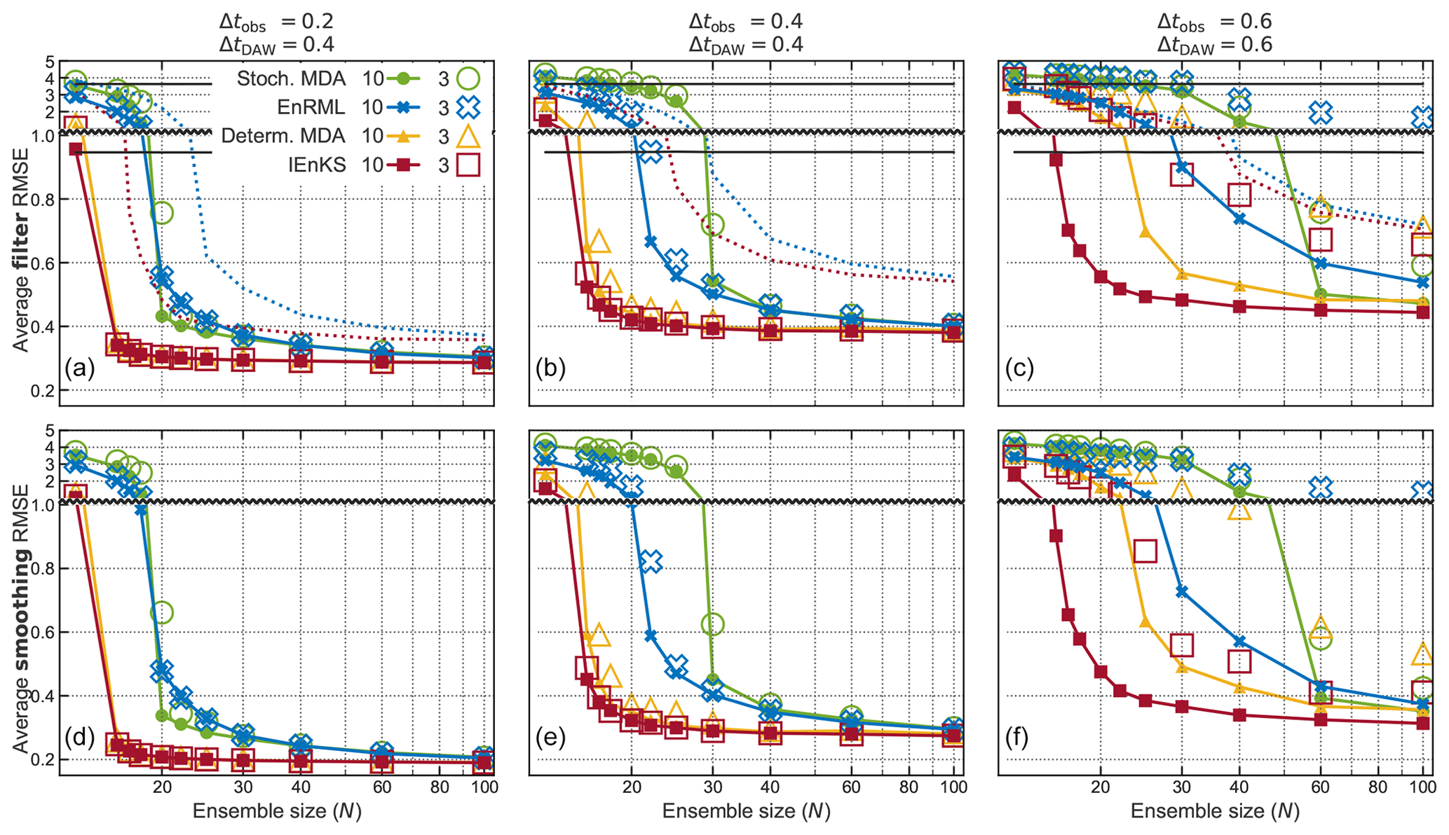
Figure 1Benchmarks of filtering (a, b, c) and smoothing (d, e, f) accuracy, in three configurations of the Lorenz 96 system, plotted as functions of N. The y-axis changes resolution at y=1. Each of the four (coloured) iterative ensemble smoothers is plotted for 3 (hollow markers) and 10 (compact markers) iterations. It can be seen that the deterministic (i.e. square-root) methods systematically achieve lower RMSE averages. For perspective, the black lines at y=3.6 and y=0.94 show the average RMSE scores of the climatological mean and of the optimal interpolation method, respectively. The dotted lines show the scores of the stochastic (blue) and deterministic (red) EnKF.
4.2 Results
A table of RMSE averages is compiled for a range of N, and then plotted as curves for each method, in Fig. 1. The upper panels report the analysis RMSE scores, while the lower panels report the smoothing RMSE scores. The smoothing scores are systematically lower, but the relative results are highly similar. Moving right among the panels increases Δtobs and thus the nonlinearity; naturally, all of the RMSE scores also increase. As a final “sanity check”, note that the performances of all of the ensemble methods improve with increasing N, which needs to be at least 15 for tolerable performance, corresponding to the rank of the unstable subspace of the dynamics plus 1 (Bocquet and Carrassi, 2017).
For experiments with Δtobs ≤0.4, using 3 iterations is largely sufficient, since its markers are rarely significantly higher than those of 10 iterations. On the other hand, for the highly nonlinear experiment where Δtobs =0.6, there is a significant advantage in using 10 iterations.
The deterministic (square-root) IEnKS and ES-MDA score noticeably lower RMSE averages than the stochastic IEnKS (i.e. EnRML) and ES-MDA, which require N closer to 30 for good performance. This is qualitatively the same result as that obtained for non-iterative methods (e.g. Sakov and Oke, 2008). Also tested (not shown) was the first-order-approximate deterministic flavour of ES-MDA (Emerick, 2018); it performed very similarly to the square-root flavour.
Among the stochastic smoothers, the one based on Gauss–Newton (EnRML) scores noticeably lower averages than the one based on annealing (ES-MDA) when the nonlinearity is strong (Δtobs ≥0.4) and for small N. A similar trend holds for the deterministic smoothers: the IEnKS performs better than ES-MDA for Δtobs =0.6. The likely explanation for this result is that EnRML and IEnKS can iterate indefinitely, while ES-MDA may occasionally suffer from not “reaching” the optimum.
Furthermore, the performance of EnRML and IEnKS could possibly be improved by lowering the step lengths to avoid causing “unphysical” states and to avoid “bouncing around” near the optimum. The tuning of the parameter that controls the step length, (e.g. the trust-region parameter and the MDA-inflation parameter) has been the subject of several studies (Chen and Oliver, 2012; Bocquet and Sakov, 2012; Ma et al., 2017; Le et al., 2016; Rafiee and Reynolds, 2017). However, our superficial trials with this parameter (not shown) yielded little or no improvement.
This paper has presented a new and simpler (on paper and computationally) formulation of the iterative, stochastic ensemble smoother known as ensemble randomized maximum likelihood (EnRML). Notably, there is no explicit computation of the sensitivity matrix , while the product is computed without any pseudo-inversions of the matrix of state anomalies. This fixes issues of noise, computational cost, and covariance localization, and there is no longer any temptation to omit the prior increment from the update. Moreover, the Levenberg–Marquardt variant is now a trivial modification of the Gauss–Newton variant.
The new EnRML formulation was obtained by improvements to the background theory and derivation. Notably, Theorem 1 established the relation of the ensemble-estimated, least-squares linear-regression coefficients, , to “average sensitivity”. Section 3.6 then showed that the computation of its action on the prior anomalies, , simplifies into a de-conditioning transformation, . Further computational gains resulted from expressing Ti in terms of the coefficient vectors, Wi, except that it also involves the “annoying” . Although it usually vanishes, the appearance of this projection is likely the reason why most expositions of the EnKF do not venture to declare that its implicit linearization of ℳ is that of least-squares linear regression. Section 3.6.3 showed that the projection is merely the result of using the chain rule for indirect regression to the ensemble space and argued that it is preferable to use the direct regression of the standard EnKF.
The other focus of the derivation was rank issues, with not assumed invertible. Using the Woodbury matrix lemma, and avoiding implicit pseudo-inversions and premature insertion of SVDs, it was shown that the rank deficiency invalidates the Hessian form of the RML update, which should be restricted to the ensemble subspace. On the other hand, the subspace form and Kalman gain form of the update remain equivalent and valid. Furthermore, Theorem 2 of Appendix A proves that the ensemble does not lose rank during the updates of EnRML (or EnKF).
The paper has also drawn significantly on the theory of the deterministic counterpart to EnRML: the iterative ensemble Kalman smoother (IEnKS). Comparative benchmarks using the Lorenz 96 model with these two and the ensemble multiple data assimilation (ES-MDA) smoother were shown in Sect. 4. In the case of small ensembles and large nonlinearity, EnRML and IEnKS achieved better accuracy than the stochastic and deterministic, respectively, ES-MDA. Similarly to the trend for non-iterative filters, the deterministic smoothers systematically obtained better accuracy than the stochastic smoothers.
As mentioned in the paper, the experimental results may be reproduced with code hosted at https://github.com/nansencenter/DAPPER/tree/paper_StochIEnS (last access: 12 September 2019).
A1 Preliminary
Proof of Theorem 1 . Assume that and that each element of Cℳ(x),x and 𝔼[ℳ′(x)] is finite. Then is a strongly consistent estimator of Cx. Likewise, almost surely, as N→∞. Thus, since for sufficiently large N, Slutsky's theorem yields almost surely. The equality to 𝔼[ℳ′(x)] follows directly from “Stein's lemma” (Liu, 1994).
The posterior ensemble's covariance, obtained using the EnKF, has the same rank as the prior's, almost surely (a.s.).
Proof. The updated anomalies, both for the square-root and the stochastic EnKF, can be written as Xa=XTa for some .
For a deterministic EnKF, for the symmetric positive definite square root of or an orthogonal transformation thereof (Sakov and Oke, 2008). Hence rank(Xa)=rank(X).
For the stochastic EnKF, Eqs. (25) and (23) may be used to show that , with . Hence, for rank preservation, it will suffice to show that Υ is a.s. full rank.
We begin by writing Υ more compactly:
From Eqs. (4), (14), and (A1), it can be seen that column n of Z follows the law . Hence, column n of Υ follows and has the sample space
Now consider, for , the hypothesis (Hn)
where Υ:n denotes the first n columns of Υ, and In: denotes the last N−n columns of IN. Clearly, H0 is true. Now, suppose Hn−1 is true. Then the columns of are all linearly independent. For column n, this means that . By contrast, from Eq. (A2), en∈𝒮n. The existence of a point in means that
Since υn is absolutely continuous with sampling space 𝒮n, Eq. (A4) means that the probability that is zero. This implies Hn a.s., establishing the induction. Identifying the final hypothesis (HN) with rank(Υ)=N concludes the proof.
A corollary of Theorem 2 and Lemma 1 is that the ensemble subspace is also unchanged by the EnKF update. Note that both the prior ensemble and the model (involved through Y) are arbitrary in Theorem 2. However, Cδ is assumed invertible. The result is therefore quite different from the topic discussed by Kepert (2004) and Evensen (2004), where rank deficiency arises due to a reduced-rank Cδ.
Conjecture 1: the rank of the ensemble is preserved by the EnRML update (a.s.), and Wi is invertible.
We were not able to prove Conjecture 1, but it seems a logical extension of Theorem 2 and is supported by numerical trials. The following proofs utilize Conjecture 1, without which some projections will not vanish. Yet, even if Conjecture 1 should not hold (due to bugs, truncation, or really bad luck), Algorithm 1 is still valid and optimal, as discussed in Sect. 3.6.3 and 3.6.4.
A2 The transform matrix
.
Proof. Let and . The following shows that S satisfies the four properties of the Moore–Penrose characterization of the pseudo-inverse of T:
-
-
STS=S, as may be shown similarly to point 1.
-
, as may be shown similarly to point 1, using Conjecture 1. The symmetry of TS follows from that of X+X.
-
The symmetry of ST is shown as for point 3.
This proof was heavily inspired by appendix A of Sakov et al. (2012). However, our developments apply for EnRML (rather than the deterministic, square-root IEnKS). This means that Ti is not symmetric, which complicates the proof in that the focus must be on X+Xi rather than alone. Our result also shows the equivalence of S+ and T in general, while the additional result of the vanishing projection matrix in the case of is treated separately in Appendix A3.
A3 Proof of Eq. (34)
Lemma 2: Ωi is invertible (provided that Wi is invertible).
Proof. We show that Ωiu≠0 for any u≠0, where . For u∈col(1), Ωiu=u. For , (Conjecture 1).
Recall that Eq. (33) was obtained by inserting Xi into the expression (Eq 30) for Ti. By contrast, the following inserts X from Eq. (35) into the expression (Eq. 29) for , yielding , and hence
Next, it is shown that, under certain conditions, the projection matrix vanishes:
Thereafter, Eq. (A11) of Appendix A4 can be used to write in terms of , reducing Eq. (A6) to (34).
The case of
In the case of , the null space of X is in the range of 1 (with probability 1; Muirhead, 1982, Theorem 3.1.4). By Lemma 2, the same applies for Xi; thus in Eq. (A5) reduces to .
The case of linearity
Let M be the matrix of the observation model ℳ, here assumed linear: ℳ(Ei)=MEi. By Eq. (A5), . But .
A4 Inverse transforms
Recall from Eq. (22) that Yi1=0. Therefore
where is defined in Eq. (24), and the identity for follows from that of . Similarly, the following identities are valid also when Wi and are swapped:
Equation (A8) is proven inductively (in i) by inserting Eq. (A7) into line 10 of Algorithm 1. It enables showing Eq. (A9), using . This enables showing Eq. (A10), similarly to Theorem 3. Note that this implies that Yi1=0 also for and hence that the identities of this section also hold with this definition. Eqs. (A9) and (A10) can be used to show (by multiplying with Ωi) that
The new and simpler EnRML algorithm was derived by PNR and further developed in consultation with GE (who also developed much of it independently) and ASS. Theorems 1 and 2 were derived by PNR, prompted by discussions with GE, and verified by ASS. The experiments and the rest of the writing were done by PNR and revised by GE and ASS.
The authors declare that they have no conflict of interest
The authors thank Dean Oliver, Kristian Fossum, Marc Bocquet, and Pavel Sakov for their reading and comments and Elvar Bjarkason for his questions concerning the computation of the inverse transform matrix.
This work has been funded by DIGIRES, a project sponsored by industry partners and the PETROMAKS2 programme of the Research Council of Norway.
This paper was edited by Takemasa Miyoshi and reviewed by Marc Bocquet, Pavel Sakov, and one anonymous referee.
Bannister, R. N.: A review of operational methods of variational and ensemble-variational data assimilation, Q. J. Roy. Meteor. Soc., 143, 607–633, 2016. a, b
Bardsley, J. M., Solonen, A., Haario, H., and Laine, M.: Randomize-then-optimize: A method for sampling from posterior distributions in nonlinear inverse problems, SIAM J. Sci. Comput., 36, A1895–A1910, 2014. a
Bocquet, M.: Localization and the iterative ensemble Kalman smoother, Q. J. Roy. Meteor. Soc., 142, 1075–1089, 2016. a
Bocquet, M. and Carrassi, A.: Four-dimensional ensemble variational data assimilation and the unstable subspace, Tellus A, 69, 1304504, https://doi.org/10.1080/16000870.2017.1304504, 2017. a
Bocquet, M. and Sakov, P.: Combining inflation-free and iterative ensemble Kalman filters for strongly nonlinear systems, Nonlin. Processes Geophys., 19, 383–399, https://doi.org/10.5194/npg-19-383-2012, 2012. a, b, c
Bocquet, M. and Sakov, P.: Joint state and parameter estimation with an iterative ensemble Kalman smoother, Nonlin. Processes Geophys., 20, 803–818, https://doi.org/10.5194/npg-20-803-2013, 2013. a, b
Bocquet, M. and Sakov, P.: An iterative ensemble Kalman smoother, Q. J. Roy. Meteor. Soc., 140, 1521–1535, 2014. a, b, c, d
Bocquet, M., Raanes, P. N., and Hannart, A.: Expanding the validity of the ensemble Kalman filter without the intrinsic need for inflation, Nonlin. Processes Geophys., 22, 645–662, https://doi.org/10.5194/npg-22-645-2015, 2015. a
Bonavita, M., Isaksen, L., and Hólm, E.: On the use of EDA background error variances in the ECMWF 4D-Var, Q. J. Roy. Meteor. Soc., 138, 1540–1559, 2012. a
Carrassi, A., Bocquet, M., Bertino, L., and Evensen, G.: Data assimilation in the geosciences: An overview of methods, issues, and perspectives, Wiley Interdisciplinary Reviews: Climate Change, 9, e535, 2018. a
Chen, Y. and Oliver, D. S.: Ensemble randomized maximum likelihood method as an iterative ensemble smoother, Math. Geosci., 44, 1–26, 2012. a, b, c, d
Chen, Y. and Oliver, D. S.: History Matching of the Norne Full Field Model Using an Iterative Ensemble Smoother-(SPE-164902), in: 75th EAGE Conference & Exhibition incorporating SPE EUROPEC, 2013a. a
Chen, Y. and Oliver, D. S.: Levenberg–Marquardt forms of the iterative ensemble smoother for efficient history matching and uncertainty quantification, Computat. Geosci., 17, 689–703, 2013b. a, b
Chen, Y. and Oliver, D. S.: Localization and regularization for iterative ensemble smoothers, Computat. Geosci., 21, 13–30, 2017. a
Emerick, A. A.: Deterministic ensemble smoother with multiple data assimilation as an alternative for history-matching seismic data, Computat. Geosci., 22, 1–12, 2018. a
Emerick, A. A. and Reynolds, A. C.: Ensemble smoother with multiple data assimilation, Computat. Geosci., 55, 3–15, 2013a. a
Emerick, A. A. and Reynolds, A. C.: Investigation of the sampling performance of ensemble-based methods with a simple reservoir model, Computat. Geosci., 17, 325–350, 2013b. a, b
Evensen, G.: Sampling strategies and square root analysis schemes for the EnKF, Ocean Dynam., 54, 539–560, 2004. a
Evensen, G.: Analysis of iterative ensemble smoothers for solving inverse problems, Computat. Geosci., 22, 885–908, 2018. a
Evensen, G.: Accounting for model errors in iterative ensemble smoothers, Computat. Geosci., 23, 761–775, https://doi.org/10.1007/s10596-019-9819-z, 2019. a
Fillion, A., Bocquet, M., and Gratton, S.: Quasi-static ensemble variational data assimilation: a theoretical and numerical study with the iterative ensemble Kalman smoother, Nonlin. Processes Geophys., 25, 315–334, https://doi.org/10.5194/npg-25-315-2018, 2018. a
Gu, Y. and Oliver, D. S.: An iterative ensemble Kalman filter for multiphase fluid flow data assimilation, SPE J., 12, 438–446, 2007. a, b, c
Hunt, B. R., Kostelich, E. J., and Szunyogh, I.: Efficient data assimilation for spatiotemporal chaos: A local ensemble transform Kalman filter, Physica D, 230, 112–126, 2007. a
Iglesias, M. A.: Iterative regularization for ensemble data assimilation in reservoir models, Computat. Geosci., 19, 177–212, 2015. a
Jardak, M. and Talagrand, O.: Ensemble variational assimilation as a probabilistic estimator – Part 1: The linear and weak non-linear case, Nonlin. Processes Geophys., 25, 565–587, https://doi.org/10.5194/npg-25-565-2018, 2018. a
Jazwinski, A. H.: Stochastic Processes and Filtering Theory, vol. 63, Academic Press, 1970. a
Kepert, J. D.: On ensemble representation of the observation-error covariance in the Ensemble Kalman Filter, Ocean Dynam., 54, 561–569, 2004. a
Kirkpatrick, S., Gelatt, C. D., and Vecchi, M. P.: Optimization by simulated annealing, Science, 220, 671–680, 1983. a
Kitanidis, P. K.: Quasi-linear geostatistical theory for inversing, Water Resour. Res., 31, 2411–2419, 1995. a
Le, D. H., Emerick, A. A., and Reynolds, A. C.: An adaptive ensemble smoother with multiple data assimilation for assisted history matching, SPE J., 21, 2–195, 2016. a
Liu, J. S.: Siegel's formula via Stein's identities, Stat. Probabil. Lett., 21, 247–251, 1994. a
Liu, Y., Haussaire, J.-M., Bocquet, M., Roustan, Y., Saunier, O., and Mathieu, A.: Uncertainty quantification of pollutant source retrieval: comparison of Bayesian methods with application to the Chernobyl and Fukushima Daiichi accidental releases of radionuclides, Q. J. Roy. Meteor. Soc., 143, 2886–2901, 2017. a
Livings, D. M., Dance, S. L., and Nichols, N. K.: Unbiased ensemble square root filters, Physica D, 237, 1021–1028, 2008. a
Lorenc, A. C.: Development of an Operational Variational Assimilation Scheme, Journal of the Meteorological Society of Japan, Series. II, 75 (Special issue: data assimilation in meteorology and oceanography: theory and practice), 339–346, 1997. a
Lorenz, E. N.: Predictability: A problem partly solved, in: Proc. ECMWF Seminar on Predictability, vol. 1, 1–18, Reading, UK, 1996. a
Luo, X., Stordal, A. S., Lorentzen, R. J., and Naevdal, G.: Iterative Ensemble Smoother as an Approximate Solution to a Regularized Minimum-Average-Cost Problem: Theory and Applications, SPE J., 20, 962–982, 2015. a
Ma, X., Hetz, G., Wang, X., Bi, L., Stern, D., and Hoda, N.: A robust iterative ensemble smoother method for efficient history matching and uncertainty quantification, in: SPE Reservoir Simulation Conference, Society of Petroleum Engineers, 2017. a
Maciejewski, A. A. and Klein, C. A.: Obstacle avoidance for kinematically redundant manipulators in dynamically varying environments, The international journal of robotics research, 4, 109–117, 1985. a
Mandel, J., Bergou, E., Gürol, S., Gratton, S., and Kasanický, I.: Hybrid Levenberg–Marquardt and weak-constraint ensemble Kalman smoother method, Nonlin. Processes Geophys., 23, 59–73, https://doi.org/10.5194/npg-23-59-2016, 2016. a
Morzfeld, M., Hodyss, D., and Poterjoy, J.: Variational particle smoothers and their localization, Q. J. Roy. Meteor. Soc., 144, 806–825, 2018. a
Muirhead, R. J.: Aspects of multivariate statistical theory, John Wiley & Sons, Inc., New York, wiley Series in Probability and Mathematical Statistics, 1982. a
Oliver, D. S.: On conditional simulation to inaccurate data, Math. Geol., 28, 811–817, 1996. a
Oliver, D. S.: Metropolized randomized maximum likelihood for improved sampling from multimodal distributions, SIAM/ASA Journal on Uncertainty Quantification, 5, 259–277, 2017. a
Oliver, D. S. and Chen, Y.: Recent progress on reservoir history matching: a review, Computat. Geosci., 15, 185–221, 2011. a
Oliver, D. S., Reynolds, A. C., and Liu, N.: Inverse Theory for Petroleum Reservoir Characterization and History Matching, Cambridge University Press, 2008. a
Ott, E., Hunt, B. R., Szunyogh, I., Zimin, A. V., Kostelich, E. J., Corazza, M., Kalnay, E., Patil, D. J., and Yorke, J. A.: A local ensemble Kalman filter for atmospheric data assimilation, Tellus A, 56, 415–428, 2004. a, b
Pires, C., Vautard, R., and Talagrand, O.: On extending the limits of variational assimilation in nonlinear chaotic systems, Tellus A, 48, 96–121, 1996. a
Raanes, P. N., Bocquet, M., and Carrassi, A.: Adaptive covariance inflation in the ensemble Kalman filter by Gaussian scale mixtures, Q. J. Roy. Meteor. Soc., 145, 53–75, https://doi.org/10.1002/qj.3386, 2019. a
Rafiee, J. and Reynolds, A. C.: Theoretical and efficient practical procedures for the generation of inflation factors for ES-MDA, Inverse Problems, 33, 115003, https://doi.org/10.1088/1361-6420/aa8cb2, 2017. a
Reynolds, A. C., Zafari, M., and Li, G.: Iterative forms of the ensemble Kalman filter, in: 10th European Conference on the Mathematics of Oil Recovery, 2006. a, b, c
Sacher, W. and Bartello, P.: Sampling errors in ensemble Kalman filtering. Part I: Theory, Mon. Weather Rev., 136, 3035–3049, 2008. a
Sakov, P. and Bertino, L.: Relation between two common localisation methods for the EnKF, Computat. Geosci., 15, 225–237, 2011. a
Sakov, P. and Oke, P. R.: Implications of the form of the ensemble transformation in the ensemble square root filters, Mon. Weather Rev., 136, 1042–1053, 2008. a, b, c
Sakov, P., Oliver, D. S., and Bertino, L.: An Iterative EnKF for Strongly Nonlinear Systems, Mon. Weather Rev., 140, 1988–2004, 2012. a, b, c, d, e, f
Sakov, P., Haussaire, J.-M., and Bocquet, M.: An iterative ensemble Kalman filter in the presence of additive model error, Q. J. Roy. Meteor. Soc., 144, 1297–1309, 2018. a, b
Stordal, A. S.: Iterative Bayesian inversion with Gaussian mixtures: finite sample implementation and large sample asymptotics, Computat. Geosci., 19, 1–15, 2015. a
Tian, X., Xie, Z., and Dai, A.: An ensemble-based explicit four-dimensional variational assimilation method, J. Geophys. Res.-Atmos., 113, https://doi.org/10.1029/2008JD010358, 2008. a
Trefethen, L. N. and Bau III, D.: Numerical linear algebra, Society for Industrial and Applied Mathematics (SIAM), Philadelphia, PA, 1997. a
van Leeuwen, P. J.: Comment on “Data assimilation using an ensemble Kalman filter technique”, Mon. Weather Rev., 127, 1374–1377, 1999. a
Zafari, M. and Reynolds, A. C.: Assessing the uncertainty in reservoir description and performance predictions with the ensemble Kalman filter, Master's thesis, University of Tulsa, 2005. a
Zupanski, M.: Maximum likelihood ensemble filter: Theoretical aspects, Month. Weather Rev., 133, 1710–1726, 2005. a
The formula (Eq. 19b) for is sometimes arrived at via a truncated Taylor expansion of ℳ around . This is already an approximation and still requires further indeterminate approximations to obtain any other interpretation than : the Jacobian evaluated at the ensemble mean.
Note that this is MDA in the sense of Emerick and Reynolds (2013a), Stordal (2015), and Kirkpatrick et al. (1983), where the annealing itself yields iterations, and not in the sense of quasi-static assimilation (Pires et al., 1996; Bocquet and Sakov, 2014; Fillion et al., 2018), where it is used as an auxiliary technique.
Their Lorenz 96 experiment only concerns the initial conditions.
Their Lorenz 96 experiment seems to have failed completely, with most of the benchmark scores (their Fig. 5) indicating divergence, which makes it pointless to compare benchmarks. Also, when reproducing their experiment, we obtain much lower scores than they report for the EnKF. One possible explanation is that we include, and tune, inflation.