the Creative Commons Attribution 4.0 License.
the Creative Commons Attribution 4.0 License.
 | 29 Mar 2019
Characterization of the South Atlantic Anomaly
Khairul Afifi Nasuddin
Mardina Abdullah
Nurul Shazana Abdul Hamid
This research intends to characterize the South Atlantic Anomaly (SAA) by applying the power spectrum analysis approach. The motivation to study the SAA region is due to its nature. A comparison was made between the stations in the SAA region and outside the SAA region during the geomagnetic storm occurrence (active period) and the normal period where no geomagnetic storm occurred. The horizontal component of the data of the Earth's magnetic field for the occurrence of the active period was taken on 11 March 2011 while for the normal period it was taken on 3 February 2011. The data sample rate used is 1 min. The outcome of the research revealed that the SAA region had a tendency to be persistent during both periods. It can be said that the region experiences these characteristics because of the Earth's magnetic field strength. Through the research, it is found that as the Earth's magnetic field increases, it is likely to show an antipersistent value. This is found in the high-latitude region. The lower the Earth's magnetic field, the more it shows the persistent value as in the middle latitude region. In the region where the Earth's magnetic field is very low like the SAA region it shows a tendency to be persistent.
- Article
(455 KB) - Full-text XML
- BibTeX
- EndNote


Electromagnetic radiation and charged particles from the Sun constantly reach the Earth (Domingos et al., 2017). Protons and electrons from the aurora, the high-speed solar wind, the radiation belts, or large solar coronal mass ejections penetrate into the Earth's atmosphere in different regions of the terrestrial magnetosphere (Sinnhuber et al., 2016). On the other hand, the Earth is surrounded by an almost spherical magnetic field, the magnetosphere, which is a natural shielding of the Earth's surface to solar and galactic cosmic-ray particles of up to several GeV (gigaelectronvolts) in energy (Ugusto et al., 2016).
The Earth's magnetic field configuration determines the trapping and distribution of energetic ionized particles (Badhwar, 1997). By far the most dominant of these fields is of core origin, accounting for over 97 % of the field observed at the Earth's surface and ranging in intensity from about 30 000 nT at the Equator to about 50 000 nT at the poles (Sabaka et al., 2002). The interaction of the solar wind with the magnetic field and atmosphere of the Earth causes, among other effects, disturbances in the ionosphere (Andalsvik and Jacobsen, 2014). The existence of the Earth's magnetic field protects the world from danger such as geomagnetic storms. But there still exists a region where the Earth's magnetic field is the weakest: this region is known as the South Atlantic Anomaly (SAA). The region arises due to the offset of the Earth's dipole of about 436 km from the Earth's center towards the direction of southeast Asia (Asikainen and Mursula, 2008).
The SAA describes a low-intensity magnetic field area which spans from east of Africa over the Atlantic Ocean to South America (Koch and Kuvshinov, 2015). Its extent area at the Earth's surface is continuously growing since instrumental intensity measurements covering part of the Southern Hemisphere and centered in South America are available (Pavón-Carrasco and De Santis, 2016). This region of weak magnetic field has expanded over time and also moved westward (Cnossen and Matzka, 2016). The existence of the SAA is linked closely with the geomagnetic field distribution (Heynderickx, 1996). From the high atmosphere and close outer space, the SAA is seen as a sort of geomagnetic hole where electric and neutral particles can flow from the Van Allen belts and from the magnetosphere into the atmosphere below (De Santis and Qamili, 2010).
In this region, the inner Van Allen radiation belt is at its nearest approach to the Earth's surface. The energetic particles captured by the geomagnetic field can reach lower altitudes forming a high-radiation region (Zou et al., 2015). This results in a larger number of energetic particles in the SAA region compared to other places.
The SAA plays a vital role for spacecraft orbiting in that region. Very few measurements have been made in this region compared to the other regions of the world (Federico et al., 2010). This research aims to characterize the SAA region based on the geomagnetic data collected from several observatories outside and inside this region.
The research focuses on characterizing the SAA by using the power spectrum analysis method. This study was motivated by the nature of the SAA, in which the area over the SAA is described by intense radiation near the Earth's surface because of the particularly weak local geomagnetic field. It appears as the preferred way in for high-energy particles in the magnetosphere, alongside the polar regions. As for satellite and spacecraft orbiting through the SAA, it will be beneficial to have an update of the magnetic field strength as it can provide the regional magnetic intensity in that area. Therefore, research carried out regarding the SAA can be used as a reference in the satellite launch and can increase knowledge of the geomagnetic field (Nasuddin et al., 2015).
Review of the SAA and power spectrum analysis
Space radiation is a very important factor affecting both humans and electronic systems (Konradi et al., 1994). The trapped radiation environment, consisting of large amounts of energetic charged particles, can be potentially harmful to human beings and space vehicles immerged in it (Qin et al., 2014). Geomagnetically trapped ionized particles, mainly electrons and protons, are a hazard to modern spaceflight (Fürst et al., 2009). Furthermore, the reduction of solar energy when passing through the atmosphere indicates that there is atmospheric turbidity (Aljawi et al., 2018). Modern society relies heavily on complex electronic systems mounted in spacecraft, which are exposed to extraterrestrial influences (Zavvari et al., 2014). There are a number of damages that spacecraft sustain while in orbit. These range from space debris, problems with the vacuum of space, various problems associated with the plasma environment, and various problems explicitly associated with the radiation environment (Heirtzler, 2002). One of the cases is that of the International Space Station, which needs additional shielding to deal with this sort of problem. Other examples are the Hubble Space Telescope that stops data collection while passing by the SAA. One SAA effect on the DORIS carrying satellites is the shift of the onboard oscillator frequency (Capdeville et al., 2016). It is known that LEO (low Earth orbit) space vehicles spend a significant part of their time in the SAA area (Grigoryan et al., 2008). Spacecraft in this area receive the biggest radiation dose, which is correlated with the intense fluxes of charged particles. Furthermore, the astronauts' condition is influenced by the increased radiation in this area. Operators who control affected space vehicles need to know how best to minimize the risk of anomalies which in many cases simply means knowing, with a high degree of accuracy, when and where to turn the systems on and off (Ginet et al., 2007).
Several research studies have been conducted regarding the SAA region. A study on the distribution of energetic particle fluxes near the SAA, based on kriging interpolation, was conducted by Suparta et al. (2013). Kriging interpolation was used in this research to forecast the dissemination of solar charged particles in the SAA area. Data from electrons with a 30 keV energy level (meped0e1) taken from the National Oceanic and Atmospheric Administration (NOAA)-15 satellite, on 8 September 2003 and 28 October in 2003, are employed (Suparta et al., 2013). The approach of ordinary kriging (OK) was selected since it is the finest linear unbiased estimator. Even so, this research also revealed a little dissymmetry of the estimate as well as variance figures meant for every model, particularly in the 0∘ longitude area. To resolve this difficulty, the robust variogram estimator usage was proposed.
Research on the radiation fields specific to the South Atlantic Anomaly was carried out by Panova et al. (1992). The research involves the explanation of the spatial as well as temporal behavior of the radiation field within the Mir space station through its passage of the South Atlantic Anomaly region. The calculation of the radiation fields on the Mir station was carried out by means of the Lyulin dosimeter. The measurements were carried out in the large diameter working compartment of the Mir station (Panova et al., 1992). The experiments were carried out to provide knowledge of the radiation fields precisely in the SAA as this provides valuable information for radiation safety for cosmonauts in the course of a long orbital flight.
One of the studies on the SAA is the New Archeomagnetic Directional Records From Iron Age Southern Africa (ca. 425–1550 CE) and Implications for the South Atlantic Anomaly by Hare et al. (2018). The new fine record confirms the researchers' earlier inferences that the SAA is the most current sign of a recurring event known as flux expulsion which has a serious effect on the manifestation of the Earth's magnetic field. Longer-term data from this region are crucial to understanding the current trend (Hare et al., 2018). In the research, a potential correlation of changes recorded in the African data accompanied by archaeomagnetism jerks was identified.
A research study on the future of the SAA in addition to implications for radiation harm in space was carried out by Heirtzler (2002). In this research, the SAA showed an important part of the harmful effects of radiation which happens close to the world's orbit. The significant plus current changes in the geomagnetic field in the South Atlantic were used in order to assess the size of the SAA up to the year 2000. This forecast pointed out that the harmful effects of radiation for spacecraft as well as mankind in space will increase significantly, covering a considerably greater geographical region than in the present day. In general, this journal provides references for those who are interested in learning about the SAA.
The method chosen to characterize the SAA is called power spectrum analysis. Research on the spectral and fractal analyses of geomagnetic and riometric antarctic observations and a multidimensional activity index was done by De Santis et al. (1997). Their study analyzed the geomagnetic and riometric data by using spectral and fractal analyses. A multidimensional index was obtained from this single-point data set to show the local and the global conditions of the magnetospheric activity. Their work is a good reference of the power spectrum analysis.
Other studies include fractal dynamics of geomagnetic storms done by Zaourar et al. (2013). In this work, the variations of the horizontal element of the Earth's magnetic field were studied. This was done to detect the scaling reaction of the temporal changeability in geomagnetic data preserved by the INTERMAGNET observatories throughout solar cycle 23. In this paper, the fractal spectral properties of the geomagnetic time series data were analyzed by applying spectral wavelet analysis techniques.
Research on applying power spectrum analysis on the occurrence of sudden storm commencements (SSCs) for solar cycles 11 to 22 was done by Mendoza et al. (2003). The data for SSCs comprise solar cycles 11 to 22 (1868–1996) (Mendoza et al., 2003). We opted for the maximum entropy method to determine the power spectral density of the SSCs time series, as well as to analyze their periodicities in the time series that were smoothed by obtaining a 13-month running mean. The current research reveals the existence of a peak for the occurrence of SSCs between 20 and 30 years.
Jian-Hui and Yao-Quan (1995) apply power spectrum analysis for spherical volumes in order to investigate clustering of the Large Bright Quasar Sample. In order to avoid the effects of galactic absorption and foreground galaxies, most of the survey regions are located at galactic latitudes higher than 40∘ N (Jian-Hui and Yao-Quan, 1995). The research was conducted to analyze the Large Bright Quasar Sample. In conclusion, the quasars of this sample are not clustered or very weakly clustered.
Stations used in the study are situated within as well as outside the SAA area. The SAA is described through the comparison of data from stations situated within the SAA area and station positions in the midlatitude area as well as the high-latitude region. This is done during the active period, which is the period of the geomagnetic storm occurrence, and the normal period, where no geomagnetic storm occurred. The active period and normal period were chosen based on the Kp index and Dst index.
Comprehensively, this makes it an intriguing subject for characterizing the SAA. It can provide a better knowledge of the Earth–space surrounding. This study can be a reference for future experimental measurements (Al-Qaisi et al., 2017). Since a number of spacecraft suffered hazards while orbiting through the SAA, it is hoped that this research can provide additional information to design spacecraft better able to withstand the damage.
2.1 Stations
Stations involved in the research were located inside and outside the SAA region. The list of the stations based on the IAGA code, geodetic latitude, and geodetic longitude can be seen in Table 1, while Fig. 1 shows their positions.

There are 15 stations involved: 5 stations were located in the SAA region, 5 stations were located in the midlatitude region, and another 5 stations were in the high-latitude region. The black circles in Fig. 1 show stations in the SAA region, the magenta circles show stations in the midlatitude region, and the blue circles represent stations in the high-latitude region.
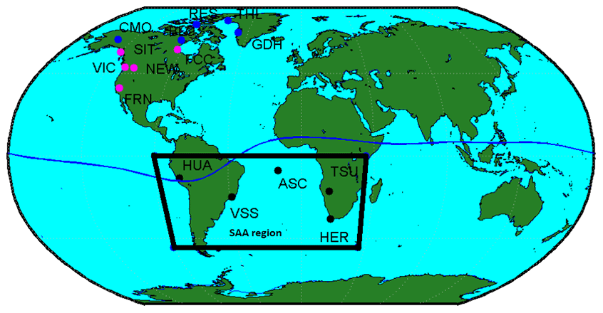
Figure 1The SAA is situated at an altitude of 200–800 km over the Earth's surface. It extends from 0 to 50∘ S and from 90∘ W to 40∘ E. The black circle is the station in the SAA region.
2.2 Power spectrum analysis and Hurst exponent
The next step is to determine the power spectral density and its scaling with respect to frequency (Hall, 2014). The spectral analysis of a time series allows one to infer something regarding the characteristic timescales of the phenomena which give rise to the observed variations (De Santis et al., 1997). A time series can be prescribed either in the time domain, as yn, or in the frequency domain in terms of the discrete Fourier transform, Ym (Malamud and Turcotte, 1999).
The power spectral density function, which is represented as Sm, whereby it is intended for a discrete time series, can be defined as represented by yn, n=1, 2, 3…, N, can be described as
It can also explain that δ is the time among consecutive n. In another situation, on behalf of a self-affine time series, the power spectral density, represented as Sm, is described to comprise a power-law dependence on frequency:
It is noted that . It can also be explained that the value of β is an estimate of the intensity of persistence in a time series. For , the Hurst exponent for a stationary fractional Gaussian noise time series is
and for a nonstationary fractional Brownian motion with 1<β≤3 it is represented by
It is important to understand the Hurst exponent, H, value. Time series with 0<H<0.5 are called antipersistent, while time series with 0.5<H<1 are called persistent (Hamid et al., 2009).
If the Hurst exponent is in the range of 0.5<H<1, it can be interpreted as both that a high value in the series will probably be followed by another high value and that the values a long time into the future will be high. A Hurst exponent in the range of 0<H<0.5 means a time series with long-term switching between high and low values in adjacent pairs, indicating a single high value may be succeeded by a low value and the following value will tend to be high, with this trend changing between high and low values and continuing for a long time into the future. A value of H equal to 0.5 implies a random series. It can also mean data are not correlated – that is, no dependence between current and past data.
2.3 Dst index and Kp index for the geomagnetic storm period and normal period
The geomagnetic storm can be known through the Dst index and Kp index. It is noted that the red line in the Dst index is the threshold for a geomagnetic storm to occur. As the Dst index is below −30 nT, it shows a geomagnetic storm occurrence. On 11 March 2011, the Dst index shows a moderate storm, occurring from 01:00 to 14:00, 18:00 to 19:00, and 21:00 to 24:00 UT. During 15:00 to 17:00 UT and on 20:00 UT a weak storm occurred. The Kp index for the active period showed that on 11 March 2011 a moderate geomagnetic storm occurred, with the Kp index showing a value of 6, and a minor geomagnetic storm occurred, with the Kp index showing a value of 5. The Kp index can be interpreted to show that a geomagnetic storm has occurred when it has a value of 5 or larger than 5.
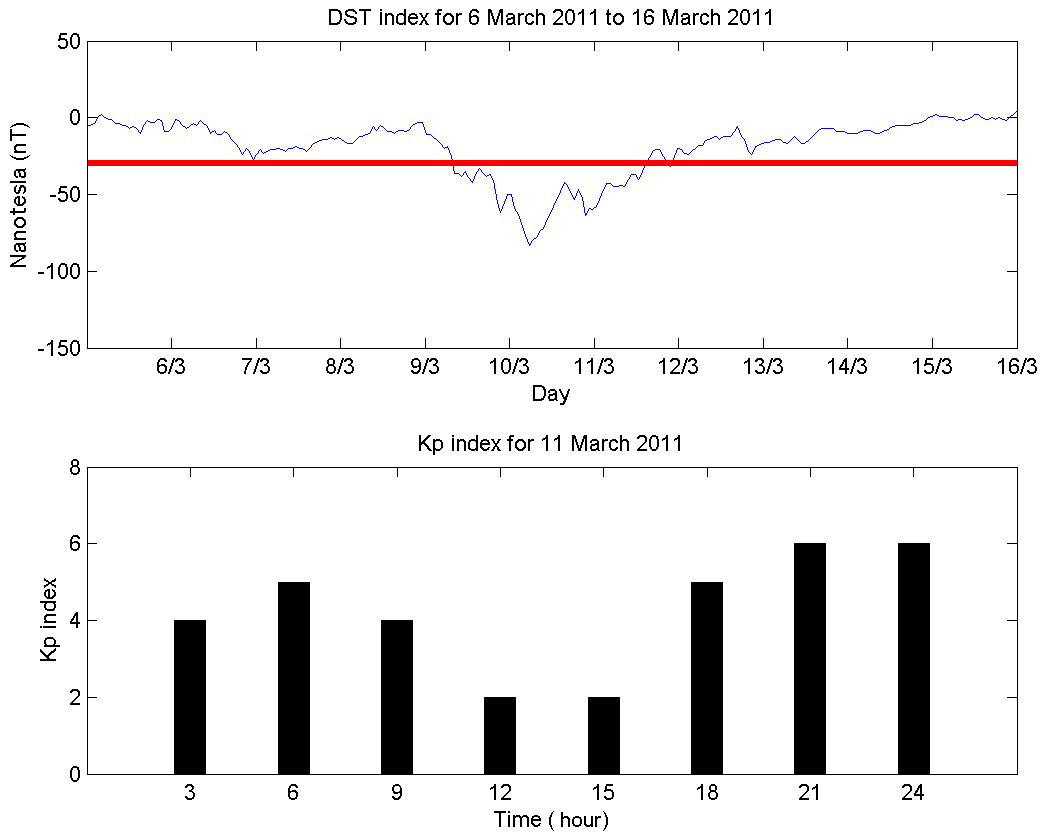
Figure 2The Dst index for 6 to 16 March 2011 and the Kp index for the active period on 11 March 2011.
For the normal period, on 3 February 2011, the Dst index indicates that no geomagnetic storm occurred. The Kp index mostly shows a value of 0 and 1, revealing no occurrence of a geomagnetic storm.
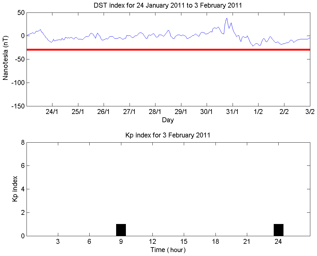
Figure 3The Dst index for 24 January to 3 February and the Kp index for the normal period on 3 February 2011.
2.4 Geomagnetic storm period and normal period
By using this method, a comparison between the active period and normal period for the stations in the SAA region, midlatitude region, and high-latitude region will be performed. The active period can be defined as a day from 01:00 until 24:00 UT where the existence of the geomagnetic storm is below −30 nT. For the normal period, it can be defined as a day from 01:00 until 24:00 UT where the value is consistently above −30 nT, indicating no geomagnetic storm occurrence.
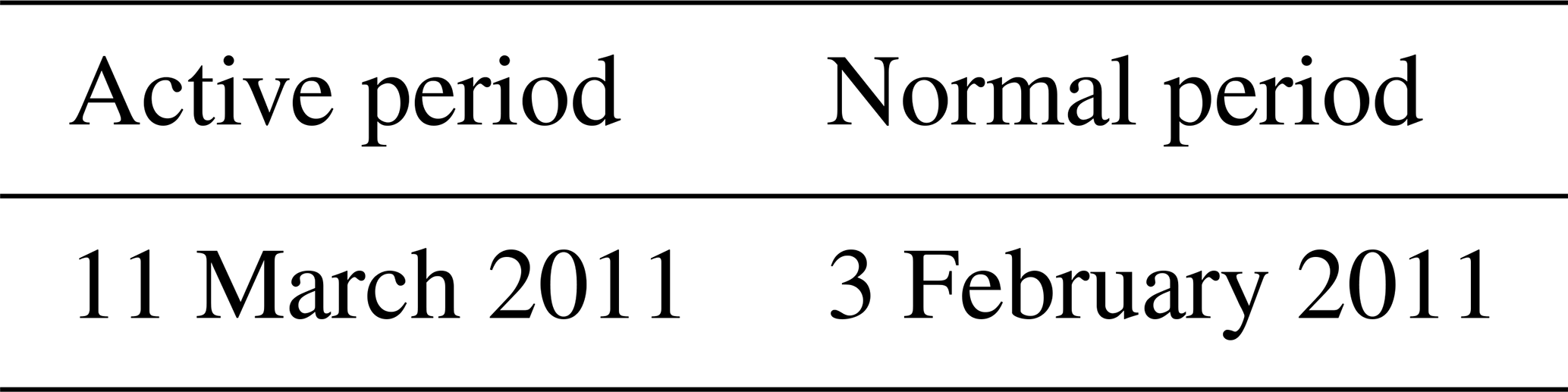
For this study, the date chosen for analysis was 3 February 2011 for a normal period and 11 March 2011 for an active period as shown in Table 2. The year 2011 was chosen to study the SAA during the rising phase of solar cycle 24.
The date for the active period, 11 March 2011, was selected because during that day the geomagnetic storm is consistently below −30 nT. Between 3 February 2011 and 11 March 2011, there are a number of geomagnetic storm occurrences. However, for the geomagnetic storm occurring between those dates, it can be seen that the existence of the geomagnetic storm is inconsistent. On 11 March 2011, the geomagnetic storm occurs consistently from 01:00 until 24:00 UT and it is the closest to 3 February 2011 based on the characteristics of the active period. On that date, 11 March 2011, the geomagnetic storm was found to occur consistently from 01:00 up to 24:00 UT according to the Dst index.
The explanation for choosing 11 March 2011 compared to other dates can be seen in more detail in Fig. 4. It can be seen through the Dst index, for example, on 1 March 2011, despite geomagnetic storm events, but it is inconsistent, unlike the geomagnetic storm on 11 March 2011.

It can be seen that on 1 March 2011 the geomagnetic storm started on that day at 13:00 and lasted until 24:00 UT, but from 01:00 to 12:00 UT no geomagnetic storm occurred. For the geomagnetic storm on 11 March 2011, it occurs from 01:00 to 24:00 UT, which is consistent throughout the day. The date of 11 March 2011 was also selected as it was closest to 3 February 2011.
2.5 H component
There are some characteristics that should be addressed regarding this work (Anwar et al., 2017). The abnormally large amplitude of the horizontal geomagnetic field component measured at the magnetic Equator is caused by the intense current flowing in the equatorial ionosphere (Hamid et al., 2013). This variation can be observed by monitoring the geomagnetic field using the global network of magnetic observatories (Hamid et al., 2010). For this research, the component of the Earth's magnetic field chosen to be analyzed is the horizontal intensity (H), since it is additionally sensitive to geomagnetic activity level. This can be studied through the beginning of a magnetic storm that is frequently described by a global sudden rise in H, which is referred to as the sudden storm commencement or SSC. Subsequent to the SSC, the H component normally remains on top of its average level for several hours. This stage is named as the initial phase of the storm. Afterwards, a great global decrease in H commences, signifying the evolution of the main phase of the storm. Among the components of the Earth's magnetic field, such as the total intensity (F), the inclination angle (I), the declination angle (D), the northerly intensity (X), the easterly intensity (Y), and the vertical intensity (Z), the horizontal intensity (H) is chosen for this reason since in this research a comparison between a period when a geomagnetic storm occurs and a period where no geomagnetic storm occurs is conducted.
Figure 5 is an example figure for power spectral density. The periodogram is obtained from station THL on 3 February 2011. The slope value is −1.6292. The value of the spectral exponent, β, is given by the negative slope of the straight line plot p(f) versus f in a log–log scale known as the periodogram.
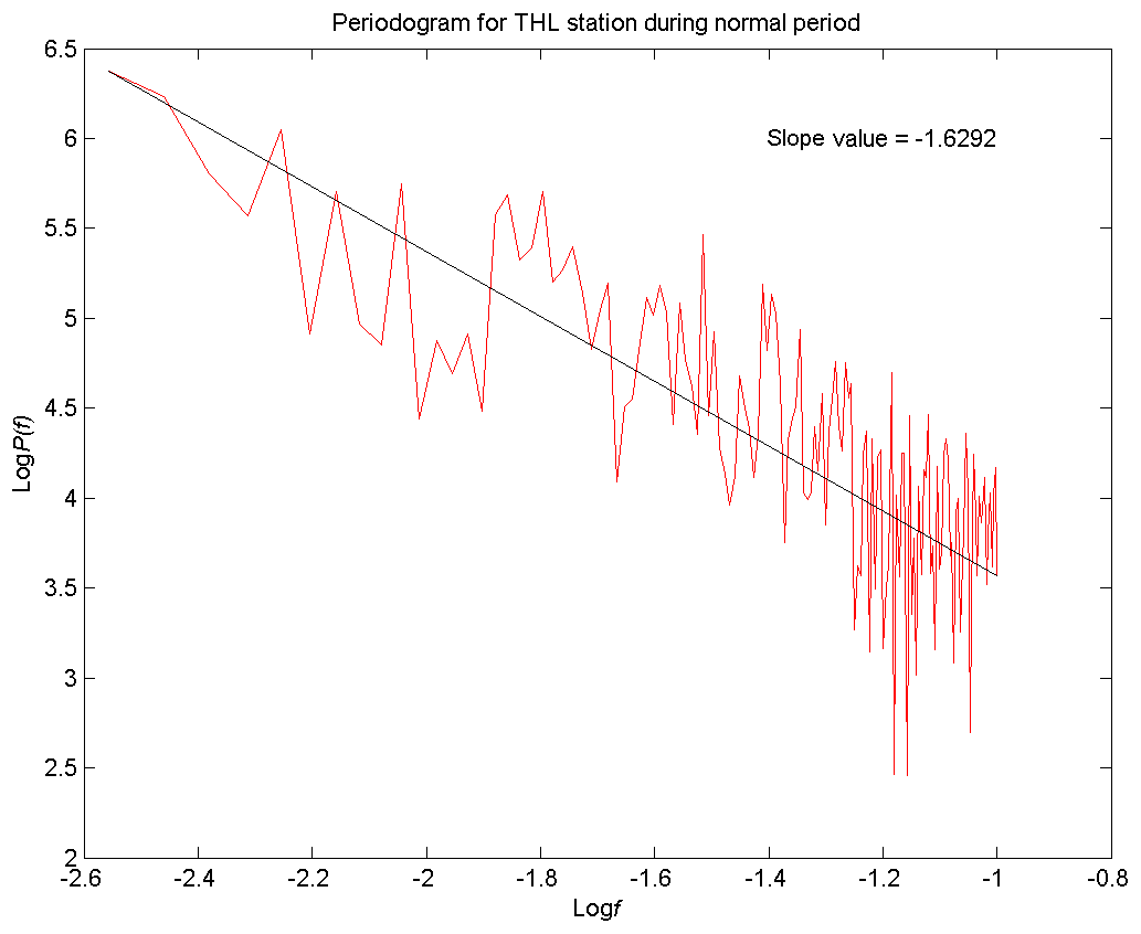
Figure 6 shows the periodogram for the high-latitude region. The red periodogram represents the active period while the blue periodogram represents the normal period. The spectral exponent, β, is in the range 1<β≤3. The spectral exponent, β, is acquired through the negative value of the slope of the best-fit straight line corresponding to the selected frequency range. The spectral exponent, β, will be applied in . The Hurst exponent, H, can determine the characteristics of the region.
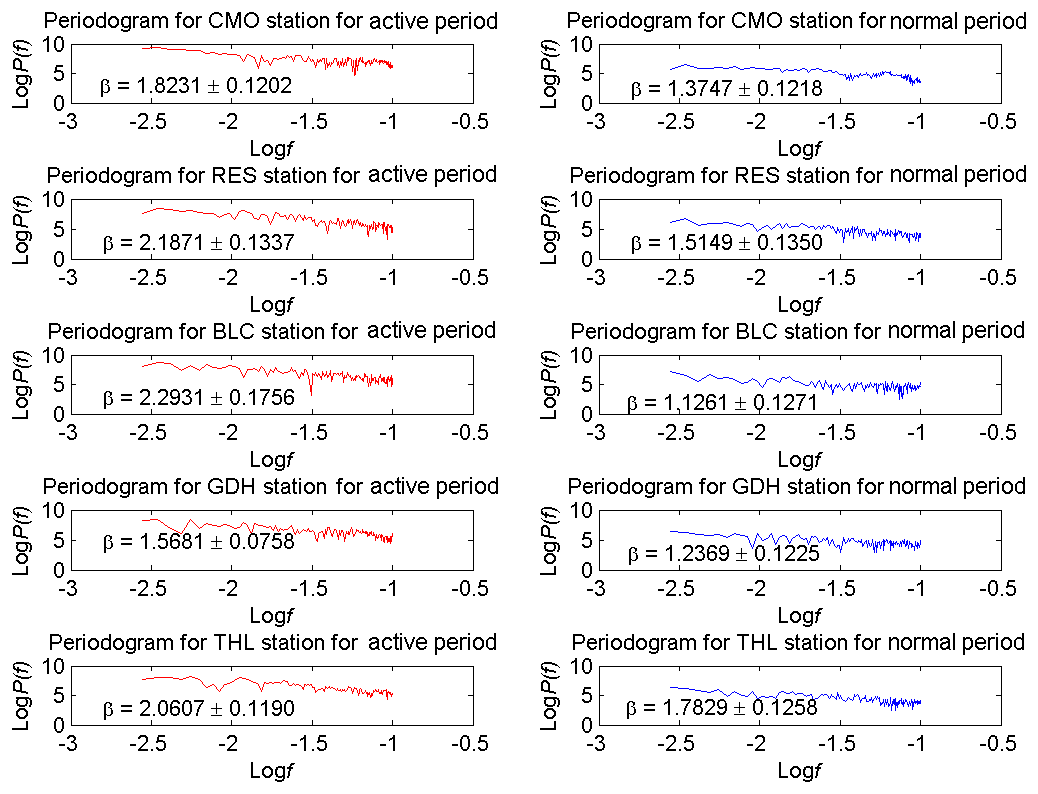
Figure 6Periodogram for the high-latitude region during the active period and normal period.
Three regions were selected for this study: the first was the high-latitude region, the second was the midlatitude region, and the third was the SAA region. A comparison between these regions was made to investigate the characteristics of the SAA region. Tables 3, 4, and 5 show the research results. Table 3 shows the results for the high-latitude region during the geomagnetic storm period (active period) and normal period, while Table 4 presents the results for the midlatitude region during the geomagnetic storm (active period) and normal period. Table 5 represents the results of the SAA region. The maximum and minimum strength of the Earth's magnetic field for stations involved in the research are also shown in the tables during active and normal periods.
Table 3The Hurst exponent as well as the maximum and minimum strength of the Earth's magnetic field during the geomagnetic storm (active period) and normal periods for stations in the high-latitude region.

As for the high-latitude region, the stations chosen were from 60 to 90∘ N. It can be seen that the Hurst exponent value is varied. During the active period, the BLC, RES, and THL stations showed persistent values of 0.6466±0.0878, 0.5936±0.0669, and 0.5303±0.0595, respectively, while the GDH and CMO stations showed antipersistent values of 0.2840±0.0379 and 0.4116±0.0601, respectively.
During the normal period, in the absence of a geomagnetic storm, the stations at high latitudes tend to record an antipersistent value. The CMO, GDH, THL, RES, and BLC station values were 0.1873±0.0609, 0.1185±0.0613, 0.3915±0.0629, 0.2574±0.0675, and 0.0631±0.0636, respectively. The obtained antipersistent values revealed a time series with long-term switching between high and low values in adjacent pairs. It means a single high value may well be succeeded by a low value and the following value will tend to be high. This trend to alternate between high and low values will continue for a long time in the future.
It can be said the persistent and antipersistent experiences by stations in the high-latitude region may be associated with the strength of the Earth's magnetic field. The value of the Earth's magnetic field is strong in the high-latitude area, thus providing a high degree of antipersistence for stations in the high-latitude region. The minimum and maximum values of the Earth's magnetic field in the active period range from 56 050 to 58 790 nT and from 57 060 to 59 440 nT, respectively. During the normal period, the minimum and maximum values of the Earth's magnetic field range from 56 910 to 59 090 nT and from 56 950 to 59 160 nT, respectively.
It can be seen that the Hurst exponent for station BLC is persistent while the Earth's magnetic field strength is high. Based on the outcome of the result, the Hurst exponent of station BLC is antipersistent when the Earth's magnetic field strength is high. This may be due to, for example, energetic particle factors. Station BLC is exposed to energetic particles especially when the geomagnetic storm occurs during the active period. Perhaps the energetic particles resulting from geomagnetic storms are able to affect the H component of the Earth's magnetic field, causing Hurst exponents in station BLC to produce the persistent value. This is because the Earth's magnetic field may change due to energetic particles originating from the geomagnetic storm. This is likely to be more concentrated in the BLC area that causes station BLC to be affected in its Hurst exponent value.
Figure 7 represent the periodogram for the midlatitude region during the active period and normal period. The midlatitude region is situated from 30 to 60∘ N.
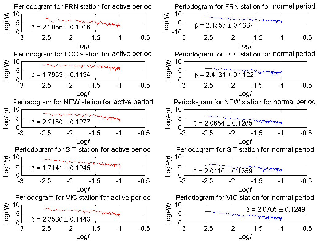
For the midlatitude region, Table 4 shows the results of the Hurst exponent value during the geomagnetic storm (active period) and normal period.
Table 4The Hurst exponent as well as the maximum and minimum strength of the Earth's magnetic field during the geomagnetic storm (active period) and normal period for station in the midlatitude region.

In the midlatitude regions, the values of the Earth's magnetic field are not as strong as in the high-latitude region. The minimum and maximum values for the Earth's magnetic field during the active period were in the range of 48 760 to 58 410 nT and 48 800 to 59 260 nT, respectively. During normal periods, the minimum and maximum values of the Earth's magnetic field ranged from 48 780 to 58 940 nT and from 48 810 to 58 980 nT, respectively. The Hurst exponent value showed a mixture of persistent and antipersistent values. The SIT and FCC stations showed antipersistent values during the active period. The values were 0.3571±0.0622 and 0.3980±0.0597. During the normal period, the values were persistent, with 0.5055±0.0680 and 0.7066±0.0561. As for the VIC station, NEW and FRN showed persistent values during the active period and normal period.
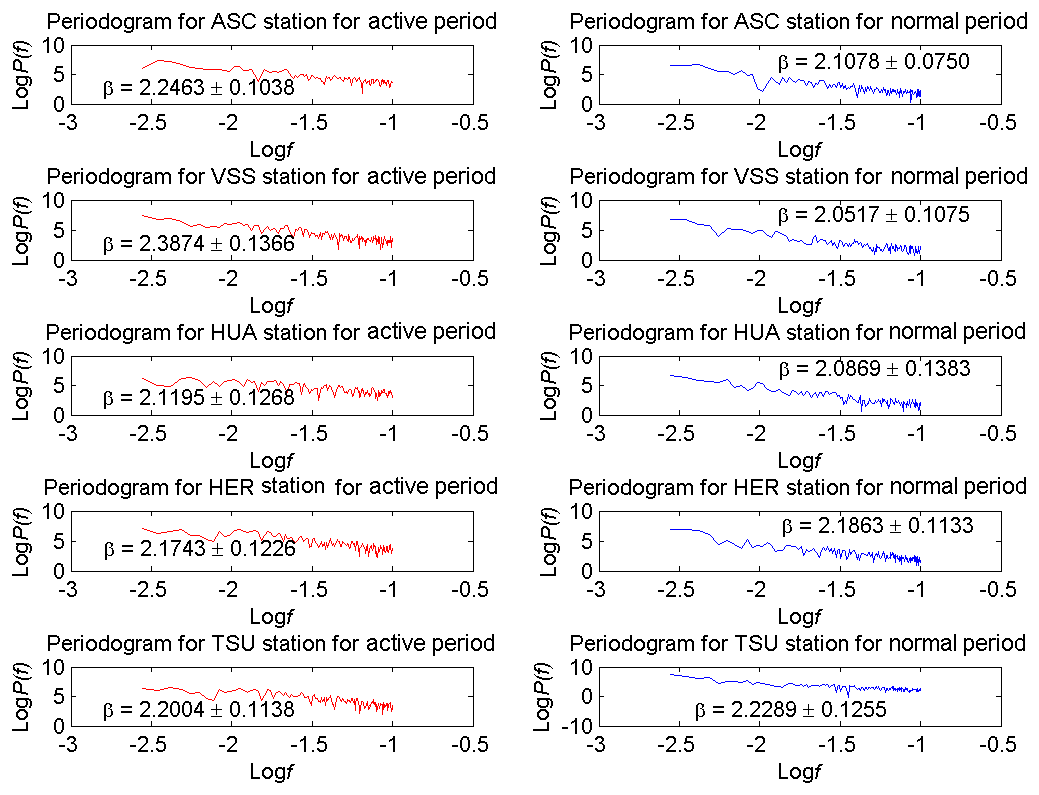
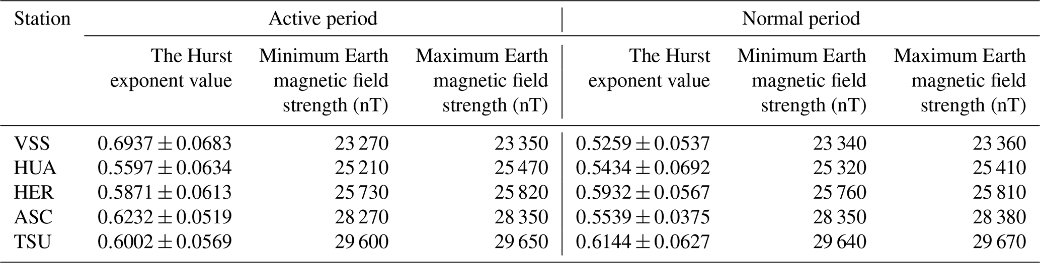
Table 5The Hurst exponent as well as the maximum and minimum strength of the Earth's magnetic field during the geomagnetic storm (active period) and normal period for the station in the SAA region.
It can be said that the value obtained in the midlatitude region differs from the value in the high-latitude region during the normal period, and the active period may be due to different values of the Earth's magnetic field. The minimum Earth magnetic field for the midlatitude region during the active period and normal period ranges from 48 760 to 58 410 nT and from 48 780 to 58 940 nT, respectively. For the maximum Earth magnetic field, values were 48 800 to 59 260 nT during the active period and 48 810 to 58 980 nT during the normal period. This is in contrast to the high-latitude region that has a higher Earth magnetic field.
In addition to the Earth's magnetic field, latitude can also affect the Hurst exponent. It can be seen that station NEW, VIC, and FRN are nearer to the SAA region, thus resulting in a persistent value of the Hurst exponent. This is because in the SAA region the value of the Hurst exponent tends to be persistent. The SIT and FCC stations are located far from the SAA region and closer to the high-latitude region where the region is more likely to be antipersistent.
Figure 8 indicates the periodogram for the SAA region during the active period as well as the normal period.
For the SAA region, Table 5 reveals the results of the Hurst exponent value during the geomagnetic storm (active period) and normal period.
In the SAA region, the value was indicated as persistent during the active period and normal period. The VSS, HUA, HER, ASC, and TSU stations during the active period were persistent, with values of 0.6937±0.0683, 0.5597±0.0634, 0.5871±0.0613, 0.6232±0.0519, and 0.6002±0.0569, respectively. During normal periods, the VSS, HUA, HER, ASC, and TSU stations recorded persistent values with a Hurst exponent of 0.5259±0.0537, 0.5434±0.0692, 0.5932±0.0567, 0.5539±0.0375, and 0.6144±0.0627, respectively.
The minimum strength of Earth's magnetic field in the SAA region during the active period and normal period ranged from 23 270 to 29 600 nT and from 23 340 to 29 640 nT, respectively. As for the maximum Earth magnetic field in the active period and normal period, the values were 23 350 to 29 650 nT and 23 360 to 29 670 nT, respectively. It could be possible to say that the SAA region experienced this characteristic because of the weak Earth magnetic field it exhibited, whereby high-energy particles in the SAA region have an effect on the value of the H component.
From the research conducted, the observations made show that the persistent and antipersistent values experienced by stations in the high-latitude region and midlatitude region, as well as the persistent tendency the SAA region experienced during the active period and normal period, could be due to the influence of the strength of the Earth's magnetic field. Regions that have a strong Earth magnetic field are more likely to be antipersistent. This can be seen in the high-latitude area. As the Earth's magnetic field decreases, it is more likely to appear persistent. This happens in the midlatitude region. Regions where the Earth's magnetic field is very low show a tendency to be persistent. This can be seen in the SAA region.
Certain factors, such as station BLC in the high-latitude region, which reveal a persistent value even when the Earth's magnetic field is high during the active period may be due to the influence of energetic particles since they occur during a geomagnetic storm. In addition, the position of a station can also affect the value of the Hurst exponent. This can be seen at stations in midlatitude regions such as NEW, VIC, and FRN which reveal a persistent value as they are much closer to the SAA region. Similarly, stations such as FCC and SIT situated in the midlatitude region, which is nearer to the high-latitude region, display an antipersistent value.
The outcomes obtained from the research show that since the SAA region is persistent during active and normal periods in this study, it can imply that a high value in the series will probably be followed by another high value and that the values for a long time into the future will also be high. It is possible for a correlation to be made on the energetic particles in the SAA region whereby a large number of energetic particles in the SAA region can also be said to remain high in the future based on the tendency of the persistent value they experience.
Data for this research can be obtained from INTERMAGNET and can be accessed at http://www.intermagnet.org/data-donnee/download-eng.php (last access: March 2019).
MA supervised the research and gave approval as well as feedback. NSAH designed the coding for the power spectrum analysis and the Hurst exponent and provided input on how the research should be done. KAN performed the research under the supervision of MA and NSAH and prepared the manuscript with contributions from all authors.
The authors declare that they have no conflict of interest.
The results presented in this paper rely on data collected at magnetic observatories. We thank the national institutes that support them and INTERMAGNET for promoting high standards of magnetic observatory practice (http://www.intermagnet.org/data-donnee/download-eng.php, last access: March 2019).
This paper was edited by Christian Franzke and reviewed by two anonymous referees.
Aljawi, O., Gopir, G., Wan Mohd Kamil, W. M. A., and Mohamad, N. S.: Estimation of the Angstrom Turbidity Parameters in the Ultraviolet Spectrum over Bangi, Malaysia, Asian J. Sci. Res., 11, 118–125, https://doi.org/10.3923/ajsr.2018.118.125, 2018.
Al-Qaisi, S., Abu-Jafar, M. S., Gopir, G. K., Ahmed, R., Omran, S. Bin, Jaradat, R., Dahliah, D., and Khenata, R.: Structural , Elastic , Mechanical and Thermodynamic Properties of Terbium Oxide: First-Principles Investigations Results in Physics Structural, elastic, mechanical and thermodynamic properties of Terbium oxide: First-principles investigations, Results Phys., 7, 709–714, https://doi.org/10.1016/j.rinp.2017.01.027, 2017.
Andalsvik, Y. L. and Jacobsen, K. S.: Observed high-latitude GNSS disturbances during a less-than-minor geomagnetic storm, Radio Sci., 49, 1277–1288, https://doi.org/10.1002/2014RS005418, 2014.
Anwar, R., Tariqul, M., Misran, N., and Gopir, G.: Development of VHF LC-Passive Filters for Multiband Transient Radio Telescope, Int. J. Appl. Inf. Technol., 1, 89–95, https://doi.org/10.25124/ijait.v1i02.1077, 2017.
Asikainen, T. and Mursula, K.: Energetic electron flux behavior at low L-shells and its relation to the South Atlantic Anomaly, J. Atmos. Solar-Terrestrial Phys., 70, 532–538, https://doi.org/10.1016/j.jastp.2007.08.061, 2008.
Badhwar, G. D.: Drift rate of the South Atlantic Anomaly, J. Geophys. Res., 102, 2343–2349, https://doi.org/10.1029/96JA03494, 1997.
Capdeville, H., Petr, S., Hecker, L., and Lemoine, J.-M.: Update of the corrective model for Jason-1 DORIS data in relation to the South Atlantic Anomaly and a corrective model for SPOT-5, Adv. Space Res., 58, 2628–2650, https://doi.org/10.1016/j.asr.2016.02.009, 2016.
Cnossen, I. and Matzka, J.: Changes in solar quiet magnetic variations since the Maunder Minimum: A comparison of historical observations and model simulations, J. Geophys. Res.-Sp. Phys., 121, 10520–10535, https://doi.org/10.1002/2016JA023211, 2016.
De Santis, A. and Qamili, E.: Equivalent Monopole Source of the Geomagnetic South Atlantic Anomaly, Pure Appl. Geophys., 167, 339–347, https://doi.org/10.1007/s00024-009-0020-5, 2010.
De Santis, A., De Franceschi, G., and Perrone, L.: Spectral and fractal analyses of geomagnetic and riometric antarctic observations and a multidimensional index of activity, J. Atmos. Solar-Terr. Phys., 59, 1073–1085, https://doi.org/10.1016/S1364-6826(96)00084-3, 1997.
Domingos, J., Jault, D., Alexandra, M., and Mandea, M.: The South Atlantic Anomaly throughout the solar cycle, Earth Planet. Sci. Lett., 473, 154–163, https://doi.org/10.1016/j.epsl.2017.06.004, 2017.
Federico, C. A., Gonçalez, O. L., Fonseca, E. S., Martin, I. M., and Caldas, L. V. E.: Neutron spectra measurements in the south Atlantic anomaly region, Radiat. Meas., 45, 1526–1528, https://doi.org/10.1016/j.radmeas.2010.06.038, 2010.
Fürst, F., Wilms, J., Rothschild, R. E., Pottschmidt, K., Smith, D. M., and Lingenfelter, R.: Temporal variations of strength and location of the South Atlantic Anomaly as measured by RXTE, Earth Planet. Sci. Lett., 281, 125–133, https://doi.org/10.1016/j.epsl.2009.02.004, 2009.
Ginet, G. P., Madden, D., Dichter, B. K., and Brautigam G, D. H.: Energetic proton maps for the South Atlantic Anomaly, IEEE Radiation Effects Data Workshop, Honolulu, HI, USA, 23–27 July 2007, 1–8, 2007.
Grigoryan, O. R., Romashova, V. V., and Petrov, A. N.: SAA drift: Experimental results, Adv. Space Res., 41, 76–80, https://doi.org/10.1016/j.asr.2007.02.015, 2008.
Hall, C. M.: Complexity signatures in the geomagnetic H component recorded by the Tromsø magnetometer (70∘ N, 19∘ E) over the last quarter of a century, Nonlin. Processes Geophys., 21, 1051–1058, https://doi.org/10.5194/npg-21-1051-2014, 2014.
Hamid, N. S. A., Gopir, G., Ismail, M., Misran, N., Hasbi, A. M., Usang, M. D., and Yumoto, K.: The Hurst exponents of the geomagnetic horizontal component during quiet and active periods, 2009 International Conference on Space Science and Communication, IconSpace – Proceedings, Negeri Sembilan, 26–27 October 2009, 186–190, 2009.
Hamid, N. S. A, Gopir, G., Ismail, M., Misran, N., Usang, M. D., and Yumoto, K.: Scaling and fractal properties of the horizontal geomagnetic field at the tropical stations of Langkawi and Davao in February 2007, AIP Conference Proceedings, Malacca, Malaysia, 7–9 December 2009, 516–519, 2010.
Hamid, N. S. A., Liu, H., and Uozumi, T.: Equatorial electrojet dependence on solar activity in the Southeast Asia sector, Antarct. Rec., 57, 329–337, https://doi.org/10.15094/00009708, 2013.
Hare, V. J., Tarduno, J. A., Huffman, T., Watkeys, M., Cottrell, R. D., Thebe, P. C., Manyanga, M., and Bono, R. K.: New Archeomagnetic Directional Records From Iron Age Southern Africa (ca. 425–1550 CE) and Implications for the South Atlantic Anomaly, Geophys. Res. Lett., 45, 1361–1369, https://doi.org/10.1002/2017GL076007, 2018.
Heirtzler, J. R.: The future of the South Atlantic anomaly and implications for radiation damage in space, J. Atmos. Solar-Terr. Phys., 64, 1701–1708, https://doi.org/10.1016/S1364-6826(02)00120-7, 2002.
Heynderickx, D.: Comparison between methods to compensate for the secular motion of the South Atlantic Anomaly, Radiat. Meas., 26, 369–373, https://doi.org/10.1016/1350-4487(96)00056-X, 1996.
Jian-Hui, T. and Yao-Quan, C.: Three dimensional power spectrum analysis of the Large Bright Quasar Sample, Chinese Astron. Astrophys., 19, 35–43, https://doi.org/10.1016/0275-1062(95)00007-F, 1995.
Koch, S. and Kuvshinov, A.: Does the South Atlantic Anomaly influence the ionospheric Sq current system? Inferences from analysis of ground-based magnetic data, Earth Planet. Sp., 67, 1–7, https://doi.org/10.1186/s40623-014-0172-0, 2015.
Konradi, A., Badhwar, G. D., and Braby, L. A.: Recent space shuttle observations of the South Atlantic Anomaly and the radiation belt models, Adv. Space Res., 14, 911–921, https://doi.org/10.1016/0273-1177(94)90557-6, 1994.
Malamud, B. D. and Turcotte, D. L.: Self-affine time series: measures of weak and strong persistence, J. Stat. Plan. Inference, 80, 173–196, https://doi.org/10.1016/S0378-3758(98)00249-3, 1999.
Mendoza, B., Valdes-Galicia, J. F., Maravilla, D., and Lara, A.: Spectral analysis results for sudden storm commencements 1868–1996, Adv. Space Res., 31, 1075–1079, https://doi.org/10.1016/SO273-1177(02)00804-9, 2003.
Nasuddin, K. A., Abdullah, M., Hamid, N. S. A., and Hasbi, A. M.: Preliminary study on the near equatorial magnetic field model and South Atlantic Anomaly, in: International Conference on Space Science Communication, Iconspace, Langkawi, Malaysia, 10–12 August 2015, 310–313, 2015.
Panova, N. A., Pftrov, V. M., and Shurshakov, V. A.: Radiation Fields Specific to the South Atlantic Anomaly, Nucl. Tracks Radiat. Meas., 20, 25–28, https://doi.org/10.1016/1359-0189(92)90080-F, 1992.
Pavón-Carrasco, F. J. and De Santis, A.: The South Atlantic Anomaly: The Key for a Possible Geomagnetic Reversal, Front. Earth Sci., 4, 1–9, https://doi.org/10.3389/feart.2016.00040, 2016.
Qin, M., Zhang, X., Ni, B., Song, H., Zou, H., and Sun, Y.: Solar cycle variations of trapped proton flux in the inner radiation belt, J. Geophys. Res.-Sp. Phys., 119, 9658–9669, https://doi.org/10.1002/2014JA020300, 2014.
Sabaka, T. J., Olsen, N., and Langel, R. a.: A comprehensive model of the quiet-time, near-Earth magnetic field: phase 3, Geophys. J. Int., 151, 32–68, https://doi.org/10.1046/j.1365-246X.2002.01774.x, 2002.
Sinnhuber, M., Friederich, F., Bender, S., and Burrows, J. P.: The response of mesospheric NO to geomagnetic forcing in 2002–2012 as seen by SCIAMACHY, J. Geophys. Res.-Sp. Phys., 121, 3603–3620, https://doi.org/10.1002/2015JA022284, 2016.
Suparta, W., Gusrizal, Mohd. Ali, M. A., and Ahmad, N.: Distribution of energetic particle fluxes in the vicinity of SAA according to Kriging interpolation, International Conference on Space Science and Communication, IconSpace, Melaka, Malaysia, 1–3 July 2013, 17–22, 2013.
Ugusto, C. A., Avia, C. N., Liveira, M. N. D. E. O., and Auth, A. F.: Signals at ground level of relativistic solar particles associated with a radiation storm on 2014 April 18, Publ. Astron. Soc. Japan, 68, 1–12, https://doi.org/10.1093/pasj/psv111, 2016.
Zaourar, N., Hamoudi, M., Holschneider, M., and Mandea, M.: Fractal dynamics of geomagnetic storms, Arab. J. Geosci., 6, 1693–1702, https://doi.org/10.1007/s12517-011-0487-0, 2013.
Zavvari, A., Islam, M. T., Anwar, R., Hasbi, A. M., Asillam, M. F., and Monstein, C.: CALLISTO Radio Spectrometer Construction at Universiti Kebangsaan Malaysia, IEEE Antennas Propag. Mag., 56, 278–288, https://doi.org/10.1109/MAP.2014.6837099, 2014.
Zou, H., Li, C., Zong, Q., Parks, G. K., Pu, Z., Chen, H., Xie, L., and Zhang, X.: Short-term variations of the inner radiation belt in the South Atlantic anomaly, J. Geophys. Res.-Sp. Phys., 120, 4475–4486, https://doi.org/10.1002/2015JA021312, 2015.