the Creative Commons Attribution 4.0 License.
the Creative Commons Attribution 4.0 License.
 | 10 Jul 2019
Data assimilation as a learning tool to infer ordinary differential equation representations of dynamical models
Julien Brajard
Alberto Carrassi
Laurent Bertino
Recent progress in machine learning has shown how to forecast and, to some extent, learn the dynamics of a model from its output, resorting in particular to neural networks and deep learning techniques. We will show how the same goal can be directly achieved using data assimilation techniques without leveraging on machine learning software libraries, with a view to high-dimensional models. The dynamics of a model are learned from its observation and an ordinary differential equation (ODE) representation of this model is inferred using a recursive nonlinear regression. Because the method is embedded in a Bayesian data assimilation framework, it can learn from partial and noisy observations of a state trajectory of the physical model. Moreover, a space-wise local representation of the ODE system is introduced and is key to coping with high-dimensional models.
It has recently been suggested that neural network architectures could be interpreted as dynamical systems. Reciprocally, we show that our ODE representations are reminiscent of deep learning architectures. Furthermore, numerical analysis considerations of stability shed light on the assets and limitations of the method.
The method is illustrated on several chaotic discrete and continuous models of various dimensions, with or without noisy observations, with the goal of identifying or improving the model dynamics, building a surrogate or reduced model, or producing forecasts solely from observations of the physical model.
- Article
(4943 KB) - Full-text XML
- BibTeX
- EndNote


1.1 Data assimilation and model error
Data assimilation aims at estimating the state of a physical system from its observation and a numerical dynamical model for it. It has been successfully applied to numerical weather and ocean prediction, where it often consisted in estimating the initial conditions for the state trajectory of chaotic geofluids (Kalnay, 2002; Asch et al., 2016; Carrassi et al., 2018). This objective is impeded by the deficiencies of the numerical model (discretrisation, approximate physical schemes, unresolved scales, and their uncertain parametrisations, e.g. Harlim, 2017) and the difficulty in matching numerical representations of the system with the observations (representation error, Janjić et al., 2018). As a result, the quality of numerical weather predictions based on a methodologically sound data assimilation method crucially depends on both the sensitivity to the initial condition due to the chaotic unstable dynamics and on model error (Magnusson and Källén, 2013).
Model errors can take many forms, and accounting for them depends on the chosen data assimilation scheme. A first class of solutions relies on parametrising model error by, for instance, transforming the problem into a physical parameter estimation problem (e.g. Bocquet, 2012; Aster et al., 2013). Other solutions are based on a weakly parametrised form of model error, for instance when it is assumed to be additive noise. Such techniques have been developed for variational data assimilation (e.g. Trémolet, 2006; Carrassi and Vannitsem, 2010), for ensemble Kalman filters and smoothers (e.g. Ruiz et al., 2013; Raanes et al., 2015), and for ensemble-variational assimilation (Amezcua et al., 2017; Sakov et al., 2018). In the weakly parametrised form, these methods should be completed by an estimation of the model error statistics (e.g. Pulido et al., 2018; Tandeo et al., 2019). Moreover, a model error's impact can be mitigated, and this is often the case in applications, by multiplicative and additive inflation (e.g. Whitaker and Hamill, 2012; Grudzien et al., 2018; Raanes et al., 2019) and by physically driven stochastic perturbations of model simulations in ensemble approaches (e.g. Buizza et al., 1999) or by stochastic subgrid parametrisations (e.g. Resseguier et al., 2017). This account is very far from exhaustive as this is a vast, multiform, and very active subject of research.
These approaches essentially seek to correct, calibrate, or improve an existing model using observations. Hence, they all primarily make use of data assimilation techniques.
1.2 Data-driven forecast of a physical system
An alternative is to renounce physically based numerical models of the phenomenon of interest and instead to only use observations of that system. Given the huge required datasets, this may seem a far-reaching goal for operational weather and ocean forecasting systems, but recent progress in data-driven methods and convincing applications to geophysical problems of small to intermediate complexity are strong incentives to investigate this bolder approach. Eventually, the perspective of putting numerical models away has a strong practical appeal, even though such a perspective may generate intense debates.
For instance, forecasting of a physical system can be done by looking up past situations and patterns using the techniques of analogues, which can be combined with present observations using data assimilation (Lguensat et al., 2017), or it can rely on a representation of the physical system based on diffusion maps that look for a spectral representation of the dataset (see chapter 6 of Harlim, 2018). An original data-driven stochastic modelling approach has been developed by Kondrashov et al. (2015). The method, recently extended to deal with multi-scale datasets (Kondrashov and Chrekroun, 2017), has been applied to successfully estimate reduced models of geophysical phenomena (see e.g. Kondrashov et al., 2018, and references therein). A fourth route relies on neural networks and deep learning to represent the hidden model and make forecasts from this representation. Examples of such an approach applied to the forecasting of low-order chaotic geophysical models are Park and Zhu (1994), who used a bilinear recurrent neural network and applied it to the three-variable Lorenz model (Lorenz, 1963, hereafter L63), Pathak et al. (2017, 2018), who use reservoir network techniques on the L63 model and on the Kuramoto–Sivashinski model (Kuramoto and Tsuzuki, 1976; Sivashinsky, 1977, hereafter KS), and Dueben and Bauer (2018), who use a neural network on a low-order Lorenz three-scale model and on coarse two-dimensional geopotential height maps at 500 hPa. The last three contributions have to resort to local reservoir networks or convolutional layers, respectively, to cope with the dimensionality of the models. However, all these representations are not mechanistic and the neural network becomes a surrogate for the hidden model. This marks a key distinction with respect to our approach where the dynamics to be determined are explicitly formulated, as will be clarified later.
1.3 Learning the dynamics of a model from its output
Data-driven techniques that seek to represent the model in a more explicit manner, and therefore with a greater interpretability, may use specific classes of nonlinear regression as advocated by Paduart et al. (2010) and Brunton et al. (2016). With a view to forecasting dynamical systems, it is possible to design neural networks in order to reflect the iterative form of a Runge–Kutta (RK) integration scheme. Wang and Lin (1998) proposed and achieved such a goal using classical activation functions, which may however blur the interpretation of the underlying dynamics. Fablet et al. (2018) went further and used a bilinear residual neural network structured so as to mimic a fourth-order RK scheme (RK4) and noise-free data. Using the Keras tool with the TensorFlow backend, their approach proved to be a very effective tool for the L63 model and to a lesser extent for the 40-variable Lorenz model (Lorenz and Emanuel, 1998, hereafter L96). In particular, they retrieved the parameters of the L63 equations to a high precision. Long et al. (2018) sought the operators of the partial differential equations (PDEs) of a physical system by identifying differentiations with convolution operators of a feed-forward neural network. They successfully applied their method to advection–diffusion problems. As opposed to our proposal, described hereafter, none of the aforementioned techniques is embedded in a Bayesian framework, making them less suitable for working with noisy and partial data.
1.4 Goal and outline
From this point on, the physical system under scrutiny will be called the reference model. It will be assumed to be known only from observations. We follow a data-driven approach inspired by the works of Paduart et al. (2010) and Fablet et al. (2018) in the sense that we will consider an observed physical reference model, which might be generated by a hidden mathematical model or process. This work is focused on either one or a combination of the following goals: (i) to build a surrogate model for the dynamics, (ii) to produce forecasts that emulate those of the reference model, and (iii) to identify the underlying dynamics of the reference model given by a mathematical model. The reference model could be totally unknown or only partially specified. To achieve these goals, we introduce a surrogate model defined by a set of ordinary differential equations (ODEs):
where is the state vector and x↦ϕ(x) is a vector field that we shall call the flow rate. For the sake of simplicity, the dynamics in this study are supposed to be autonomous, i.e. do not explicitly depend on time. Our technique seeks a fit ϕ given observations of the reference model. This is a rather general representation since, for instance, PDEs can be discretised into ODEs. We will restrict ourselves to the case where ϕ is at most quadratic in . The numerical integration of Eq. (1) could be based on any RK scheme, but should additionally rely on the composition of such integration steps. As a result, quite general resolvents of Eq. (1) can be built (the resolvent is the model, i.e. the flow rate, integrated in time over a finite time interval).
Importantly, we will not require any machine learning software tool since the adjoint of the model resolvent can be derived without a lot of effort. As opposed to the contributions mentioned in the previous subsections, we embed the technique in a data assimilation framework. From a data assimilation standpoint, the technique can be seen as meant to deal with model error (with or without some prior on the model) and it naturally accommodates partial and noisy observations. Moreover, we will build representations of the dynamics that are either invariant by spatial translation (homogeneous) and/or local (i.e. the flow rate of a variable xn only depends on neighbouring variables whose perimeter is defined by a stencil). These properties make our technique scalable and thus potentially applicable to high-dimensional systems.
In Sect. 2, we present model identification as a Bayesian data assimilation problem. We first choose an ODE representation of the dynamics, introduce a nonlinear regressor basis, and define the integration schemes we will work with. We describe the local and homogeneous representations as physically based simplifications of the most general case, and we derive the gradient of the problem's cost function based on these representations. We then introduce the Bayesian problem and the resulting cost function used for joint supervised learning of the optimal representation and estimation of the state trajectory. The latter is the standard goal of data assimilation, while the former is that of machine learning. Our approach blends them together using the formalism of data assimilation.
In Sect. 3, we discuss several theoretical issues: the prior of the model, the convergence of the training step, the connection with numerical analysis of integration schemes, the connection with deep learning architectures, and, finally, the pros and cons of our approach.
In Sect. 4, we illustrate the method with several low-order chaotic models (L63, L96, KS, and a two-scale Lorenz model) of various sizes, from a perfectly identifiable model, i.e. where the model used to generate the dataset can be retrieved exactly, to a reduced-order model where the model used to generate the dataset cannot be retrieved exactly, using full or partial, noiseless, or noisy observations. Conclusions are given in Sect. 5.
2.1 Ordinary differential equation representation
Our surrogate model is chosen to be represented by an ODE system as described by Eq. (1). We additionally assume that the flow rate can be written as
where is a matrix of real coefficients to be estimated and is a map that defines regressor functions of x. is the latent space of the regressors in which the flow rate is linear.
In the absence of any peculiar symmetry, we choose this map to list all the monomials up to second order built on x, i.e. the constant, linear, and bilinear monomials. Let us call the set of all variable indices and 𝒫 the set of all pairs of variable indices. We introduce the augmented state vector
extend 𝒟 to , and define as the distinct pairs of variable indices in .
As a result, the regressors are compactly defined by
where the scalars in the bracket are the entries of the vector r(x). We count
regressors, i.e. the cardinal of . For instance, a model with three variables, x0,x1, and x2, such as L63, has 10 such regressors:
Higher-order regressors, as well as regressors of different functional forms, could be included as in Brunton et al. (2016). However, it is important to keep in mind that we do not seek an expansion of the resolvent of the reference model, but of the flow rate ϕA. As a consequence, higher-order products of the state variables are anyhow generated by the integration schemes and their composition. It is worth mentioning that nonlinear regressions are not widespread in geophysical data assimilation. We are nonetheless aware of at least one noticeable exception that extends traditional Gaussian-based methods (Hodyss, 2011, 2012).
2.2 Local and homogeneous representations
At least two useful simplifications for the ODEs could be exploited if the state x is assumed to be the discretisation of a spatial field.
2.2.1 Locality
First, we use a locality assumption based on the physical locality of the system: all multivariate monomials in the ODEs have variables xn that belong to a stencil, i.e. a local arrangement of grid points around a given node. This can significantly reduce the number of bilinear monomials in r(x). We assume that sn is the stencil around node n, the pattern being the same for all nodes except the last one. For the node Nx corresponding to the extra variable , we assume that its stencil consists of all the Nx+1 nodes. We then define as the sub-set of all pairs (n,m) of variables for which m∈sn. The set of required monomials can therefore be reduced to
Under these conditions, A becomes sparse. Indeed, for each node n, we assume that , the time derivative of xn, is impacted only by linear terms xm such that m∈sn and quadratic terms xmxl such that m∈sn, l∈sn, and m∈sl. However, to keep a dense matrix, we choose to compactly redefine and shrink A by eliminating all a priori zero entries due to the locality assumption. The number of columns of A is then significantly reduced from Np to Na. As a consequence of this redefinition of A, the matrix multiplication in between A and r(x) must be changed accordingly. Nonetheless, the operation that assigns coefficients in A to the monomials in r(x) remains linear, and we write it as
Let us take the example of a one-dimensional extended space as those used in Sect. 4. The domain is supposed to be periodic (circle) and the nodes are indexed by . Recall that the node of index Nx is associated with the extra {1}. For , the stencil sn is defined as the set of 2L+1 nodes of index , plus the extra node of index Nx. The stencil consists of all the nodes, i.e. 𝒟. We assume . In that case r(x) as defined by Eq. (7) has monomials. For instance, there are 161 such regressors for a 40-variable model defined on a circular domain, such as L96, with L=2:
The row [A]n of the dense A contains the following coefficients for each . First there are 2L+2 regressors built with {1} (the constant and linear regressors). Second, we consider the square monomials with m∈sn, i.e. whose number is 2L+1. Then we consider those separated by one space step, whose number is 2L, followed by those separated by two space steps whose number is 2L−1, and so on until a separation of L is reached. Quadratic monomials of greater separation are discarded since they do not belong to a common stencil as per the above definition reflecting the locality assumption. Hence there is a total of coefficients per grid cell.
In Appendix A, we show in the one-dimensional space case how to compute the reduced form of the product between A and r(x), assuming locality. This type of technical parametrisation is required for a parsimonious representation of the control variables, i.e. the coefficients of A, and is key for a successful implementation with high-dimensional models.
Note that this locality assumption is hardly restrictive. Indeed, owing to the absence of long-range instantaneous interactions (which are precluded in geophysical fluids), farther distance correlations between state variables can be generated by small stencils in the definition of ϕA through time integrations. This would not prevent potential specific long-distance dependencies (such as teleconnections).
2.2.2 Homogeneity
Furthermore, a symmetry hypothesis could optionally be used by assuming translational invariance of the ODEs, called homogeneity in the following. Because our control parameters, i.e. the coefficients of A, parametrise the flow rate, the symmetry simply translates into the rows [A]n of the dense A being the same for all n. Hence A simply becomes a vector in .
Let us enumerate its coefficients in the case of the L96 model with L=2 and assuming both locality and homogeneity. The coefficients are partitioned into A(0) for the bias, for the linear sector, and for the bilinear sector. In the linear sector, is the relative position with respect to the current grid point. In the bilinear sector, l,m are the relative positions with respect to the current grid point of the two variables in the product. Proceeding in the same way we counted them, the Na=18 coefficients of A are
Note that while both constraints, locality and homogeneity, apply to the ODEs, they do not apply to the states per se. For instance, ODEs for discretised homogeneous two-dimensional turbulence satisfy both constraints and yet generate non-uniform flows.
For realistic geofluids, the forcing fields (solar irradiance, bathymetry, boundary conditions, friction, etc.) are heterogeneous, so that the homogeneity assumption should be dropped. Nonetheless, the fluid dynamics part of the model would remain homogeneous. As a result, a hybrid approach could be enforced.
2.3 Integration scheme and cycling
The reference model will be observed at time steps tk, indexed by integer . Hence, we need to be able to express the resolvent of the surrogate model from tk to tk+1. We assume that is a multiple of the integration time step of the surrogate model, , where h is the integration time step and is the number of integrations. The time steps can be uneven, which is reflected in the dependence of on k. Hence, the resolvent of the surrogate model from tk to tk+1 can be written as
i.e. the integration of Eq. (1) from tk to tk+1 using the representation Eq. (2).
We define intermediate state vectors in between : xk,l is the state vector defined at time for , as the result of l compositions of fA on xk: . Figure 1 is a schematic of the composition of the integration steps, along with the state vectors xk and xk,l.

Figure 1 Representation of the data assimilation system as a hidden Markov chain model and of the model resolvents and fA.
The operator fA is meant to be an explicit numerical integration scheme. In the following, we shall consider an RK scheme applied to , with NRK steps. This number of steps coincides with the accuracy of the schemes that we will consider: first order for the Euler scheme, second order for RK2, and fourth order for RK4 (, and 4, respectively). Provided the dynamics are autonomous, a general RK scheme reads as
where the coefficients βi and αi,j entirely specify the scheme and . Note that αi,j are zero for j≥i, so that Eq. (12b) can be computed iteratively from k0 to , followed by the sum Eq. (12a) to get fA(x).
In the following, h will be absorbed into the definition of A and hence ϕA, so that we can take h=1 without loss of generality.
2.4 Bayesian analysis
We consider a sequence of observation vectors of the physical system at tk indexed by . The system state is observed through
where Hk is the observation operator at time tk. The observation error ϵk will be assumed to be Gaussian with zero mean and covariance matrix rk. It is also assumed to be white in time. The flow rate ϕA is given by the approximation Eq. (2), so that the resolvent FA of the surrogate model should also be considered an approximation of the reference model's resolvent. Hence, we generalise Eq. (11) to
where ηk are unbiased Gaussian errors of covariance matrices Qk, supposed to be white in time and uncorrelated from the observation errors. Note that, in all generality, the state space of the surrogate model does not have to match that of the reference model. We will nonetheless take them to coincide here merely for simplicity.
With the goal of identifying a model or building a surrogate of the reference one, we are interested in estimating the probability density function (pdf) , where y0:K stands for all observations in the window [t0,tK]. To obtain a tractable expression for this conditional likelihood, we need to marginalise over the state variables x0:K within the window:
An approximate maximum a posteriori for A could be obtained by using the Laplace approximation of this integral, which would require finding the maximum of
Nonetheless, maximising Eq. (16) rigorously yields the maximum a posteriori of the joint variables . The cost function associated with this joint pdf is by definition . Because Eq. (14) is Markovian and given the Gaussian form of both model and observational errors, the cost function reads as
up to a constant depending on Q1:K and r0:K only. The vector norm ∥z∥P is defined as . This is the cost function of a weak constraint 4D-Var (see Sect. 2.4.3.2 of Asch et al., 2016) with A and x0:K as control variables.
In the case where the reference model is fully and directly observed, i.e. Hk≡Ix, and in the absence of observation noise, i.e. rk≡0, we have and the cost function simplifies to
where y0:K is the fully and perfectly observed state trajectory of the reference model. This is notably similar to a traditional least-square function used in machine and deep learning regression. This connection between machine learning and data assimilation cost functions had been previously put forward by Hsieh and Tang (1998) and Abarbanel et al. (2018), although in a different form. Reciprocally, when the aforementioned hypotheses of noiseless and complete observations do not hold, Eq. (17) can be seen as a natural data assimilation extension of Eq. (18). Note that Eq. (18) only depends on the sequence Q1:K. If, in addition, the dependence on is neglected in Eq. (18), then the maximum a posteriori should not depend on a global rescaling of Q1:K.
The data assimilation system is represented in Fig. 1 as a hidden Markov chain model. This Bayesian view highlights the choice that must be made for r0:K and/or Q1:K and provides an interpretation in terms of errors. Furthermore, one could implement an objective estimation of these error statistics as in Pulido et al. (2018).
2.5 Gradients and adjoint of the representation
To efficiently minimise the cost function Eq. (17) with a gradient-based optimisation tool, we need to analytically derive the gradient of Eq. (17) with respect to both A and x0:K. As for x0:K, we have
where for and for ; is the tangent linear operator of the resolvent computed at xk for ; is the tangent linear operator of the observation operator Hk computed at xk for . As for A, we have
assuming x0 is independent of A. Hence, a key technical aspect of the problem is to compute the tangent linear and adjoint operators required by these gradients. In this paper, we assume that the adjoints of the tangent linear operators of the observation operators are known, for instance if the latter are linear as in Sect. 4.
The computations of the gradients and the required adjoints are developed in Appendix B. These technicalities can be skipped since they are not required to understand the method. Nonetheless, they are critical to its numerical efficiency.
In this section, we discuss the prior pdf p(A), the optimisation of the cost function , and the connections with deep learning techniques.
3.1 Prior information on the reference model
The goal is either to reconstruct an ODE for the reference model, characterised by the coefficients A through ϕA, or to build a surrogate model of it. The estimation of x0:K is then accessory even though factually critical to the estimation of A. The alternative would have been to consider the estimation of x0:K as the primary problem, under model error of a prescribed ODE form, the estimation of A becoming accessory. In both cases, but particularly in the latter one, one may benefit from an informative prior pdf p(A).
The prior pdf p(A) can be used to encode any prior knowledge on the reference model, such as pieces of it that would be known. Indeed, p(A) can formally quantity the uncertainty associated with any part of the surrogate model. For instance, assume that the reference model is partially identifiable, which means that part of the reference model could be represented by an up to bilinear flow rate of the form Eq. (2) and Eq. (4). Moreover, assume that there is one such part of the reference model which is known, i.e. that elements of A are actually known, while others need to be estimated. Then, the known coefficients can formally be encoded in p(A) with Dirac factors. In practice it could be implemented as a constrained optimisation problem, for instance using an augmented Lagrangian, in order to avoid significantly altering the gradients with respect to A. More generally, assigning a non-trivial prior likelihood, such as a Gaussian one for A, is certainly appealing but may not be practical.
3.2 Numerical optimisation: issues and solutions
The success of the optimisation of depends above all on the ability to evaluate it robustly. In particular, it depends on the stability of the numerical integration scheme . In this paper, we chose to rely on one-step explicit schemes which are much simpler to describe and efficient to integrate (a family to which the RK schemes of any NRK belong). These schemes are 0-stable, which means that the finite time error growth goes to zero as the integration step goes to zero. But, as a major drawback, they have a limited absolute (or A-)stability domain (see e.g. chapters 5 and 6 of Gautschi, 2012). For a given state trajectory, there exists a stability domain out of which the evaluation of is hazardous. A failure to evaluate the cost function also depends on the number of integration steps since the instabilities are likely to increase exponentially with .
This says that, in the absence of a strong prior p(A), it is safer to start with A=0 likely to lie close to 𝒟s. Alternatively, if stability constraints are known about A, they could be encoded in p(A). It also says that we should strike an empirical compromise between the composition numbers and the easiness in evaluating . On the one hand, the larger , the more the iterates of A in the optimisation must be kept confined in 𝒟s. On the other hand, the longer , the broader the class of achievable resolvents and hence the ability to build a good surrogate. Moreover, the higher the stability of the integration scheme, the larger 𝒟s, and the easier the optimisation in spite of an increase in its numerical cost.
As for the sensitivity on K, the longer the time window, the more observations are available to constrain the problem. However, the longer K, the higher the chances of having a significant instability: the chances of a successful integration typically decrease exponentially with the length K.
This stability issue can be somehow alleviated by normalising the observations yk by their mean and variance in order to avoid excessively large value ranges of the regressors. This will not change the fundamental stability of the schemes, yet may delay the occurrences of instabilities due to the nonlinear terms.
Moreover, instabilities can significantly be mitigated by replacing the monomials with smoothed or truncated ones:
One can for instance choose , in order to cut off too large values of and hence delay the growth of instabilities. The parameter λ>0 is roughly chosen as the typical maximum amplitude of as approximately inferred from the observations. If tanh is deemed to be numerically too costly, one can choose instead or more generally , with a small trend.
This latter change in variables is the one implemented for all numerical applications described in Sect. 4, together with the normalisation. From these experiments, we learned that these tricks often turned critical in the first iterates of the optimisation when the estimate of A progressively migrated to the A-stability domain. After a few iterations, however, the integrations are stabilised and the nonlinear regime of the truncations in Eq. (21) is not tapped into anymore.
3.3 Connection and analogies with deep learning architectures
It has recently been advocated that residual deep learning architectures of neural networks can roughly be interpreted as dynamical systems (e.g. Weinan, 2017; Chang et al., 2018). Each layer of the network contributes marginally to the output, so that there exists an asymptotic continuum limit representation of the neural network. Furthermore, as mentioned in the introduction, Wang and Lin (1998) and Fablet et al. (2018) have shown that the architecture of the network can follow that of an integration scheme.
By contrast, we have started here from a pure dynamical system standpoint and proposed to use data assimilation techniques. In order to explore complex model resolvents, applied to each interval between observations, we need the composition of Nc integration steps. In particular, this allows the resolvent to exhibit more realistic long-range correlations. Even when using a reasonably small stencil, long-range correlations will arise as a result of the integration steps. Nonetheless, the stencil might not be too small so as to model discretised higher-order differential operators. As noted by Abarbanel et al. (2018), each application of fA could be seen as a layer of the neural network. Moreover, within such a layer, there are sublayers corresponding to the steps of the integration scheme. The larger Nc is, the deeper this network is, and the richer the class of resolvents is to optimise on.
Following this analogy, the analysis step where is optimised can be called the training phase. Backpropagation in the network, as coined in machine learning (Goodfellow et al., 2016), corresponds to the computation of the gradient of the network with respect to A and of the model adjoint derived in Sect. 2. This is a shortcut for the use of machine learning software libraries such as TensorFlow or PyTorch (see Appendix C for a brief discussion).
Because of our complete control of the backpropagation, we hope for a gain in efficiency. However, our method does not have the flexibility of deep learning through established tools. For instance, addition of extra parameters, adaptive batch normalisation, and dropouts are not granted in our approach without further considerations.
Convolutional layers play the role of localisation in neural architecture. In our approach this role is played by the locality assumption and its stencil prescription. Recall that a tight stencil does not prevent longer-range correlations that are built up through the integration scheme and their composition. This is similar to stacking several convolutional layers to account for multiple scales from the reference model which the neural network is meant to learn from.
Finally, we note that, as opposed to most practical deep learning strategies with a huge amount of weights to estimate, we have reduced the number of control variables (i.e. A) as much as possible.
4.1 Model setup and forecast skill
In this section, we shall consider four low-order chaotic models defined on a physical one-dimensional space, except for L63, which is 0-dimensional. They will serve as reference models.
-
The L63 model as defined by the ODEs:
with the canonical values . Its Lyapunov time1 is about 1.10. Besides its intrinsic value, this model is introduced for benchmarking against Fablet et al. (2018). It is integrated using an RK4 scheme with δtr=0.01 as the integration time step.
-
The L96 model as defined by ODEs defined over a periodic domain of variables indexed by where Nx=40:
where , , , and F=8. This model is an idealised representation of a one-dimensional latitude band of the Earth's atmosphere. Its Lyapunov time is 0.60. It is integrated using the RK4 scheme and with δtr=0.05.
-
The KS model, as defined by the PDE:
over the periodic domain on which we apply a spectral decomposition with Nx=128 modes. The Lyapunov time of our KS model is 10.2 time units. This model is of interest because, even though it has dynamical properties comparable to that of L96, it is much steeper, so that much more stringent numerical integration schemes are required to efficiently integrate it. It is defined by a PDE, not an ODE system. It is integrated using the EDTRK4 scheme (Kassam and Trefethen, 2005) and δtr=0.05.
-
The two-scale Lorenz model (L05III, Lorenz, 2005) is given by the two-scale ODEs:
for with Nx=36 and with Nu=360. The indices apply periodically over their domain; m∕10 stands for the integer division of m by 10. We use the original values for the parameters: c=10 for the timescale ratio, b=10 for the space-scale ratio, h=1 for the coupling, and F=10 for the forcing. When uncoupled (h=0), the Lyapunov time of the slow variables x sector of the model Eq. (25) is 0.72, which will be the key timescale when focusing on the slow variables (see e.g. Carlu et al., 2019).
This model is of interest because the variable u is meant to represent unresolved scales and hence model error when only considering the slow variables x. For this reason, it has been used in data assimilation papers focusing on estimating model error (e.g. Mitchell and Carrassi, 2015; Pulido et al., 2018). It is integrated with an RK4 scheme and δtr=0.005 since it is steeper than the L96 model.
The numerical experiments consist of three main steps. First, the truth is generated, i.e. a trajectory of the reference model is computed. The reference model equations are supposed to be unknown, but the trajectory is observed through Eq. (13) to generate the observation vector sequence y0:K.
Next, estimators of the ODE model and state trajectory x0:K are learned by minimising the cost function . We choose to minimise it using an implementation of the quasi-Newton BFGS algorithm (Byrd et al., 1995), which critically relies on the gradients obtained in Sect. 2. The default choices for the initial ODE model are A=0 and x0:K defined as the space-wise linear interpolation of y0:K. Note that the minimisation could converge to a local minimum, which may or may not yield satisfactory estimates.
Finally, we can make forecasts using the tentative optimal ODE model A⋆ obtained from the minimisation. With a view to comparing it to the reference model used to generate the data, we will consider a set of forecasts with (approximately) independent initial conditions. Both the reference model and the surrogate one will be forecasted from these initial conditions. The departure from their trajectories, as measured by a root mean square error (RMSE) over the observed variables, will be computed for several forecast lead times. The RMSE is then averaged over all the initial conditions. We will also display the state trajectories of the reference and surrogate models starting from one of the initial conditions.
The integration time step of the truth (reference model) is δtr over the time window [t0,tK]. This parameter only matters for the reference model integration since only the training time steps and the output of the model y0:K (which may include knowledge of the observation operator) are known to the observer.
The integration time step of the surrogate model within the training time window [t0,tK] is δta. It is assumed to be an integer divisor of the training time step , supposed to be constant, i.e. Δt∕δta is a constant integer and the number of compositions Nc, and that is why the index k on has been dropped. The integration time step of the surrogate model within the forecast time window is denoted δtf. Note that δta and δtf can be distinct and that they are critical to the stability of the training and the forecast step, respectively.
The three steps of the numerical experiments are depicted in Fig. 2. Except when explicitly mentioned, the prior p(A) is disregarded, which means that no explicit regularisation on A is introduced.
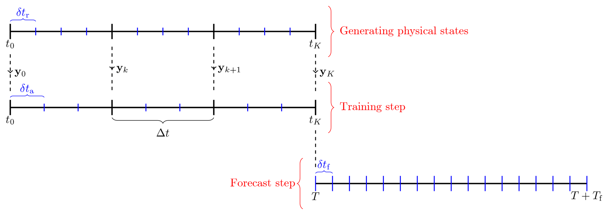
Figure 2 Schematic of the three steps of the experiments, with the associated time steps (see main text). The beginning of the forecast window may or may not coincide with the end of the training window. The lengths of the segments δtr, δta, and δtf are arbitrary in this schematic.
4.2 Inferring the dynamics from dense and noiseless observations: perfectly identifiable models
In the first couple of experiments, we consider a densely observed2 reference model with noiseless observations. In this case, Hk is the identity operator, i.e. each grid point value is observed, and rk≡0 so that a uniform rescaling of the Qk, all chosen to be Ix, is irrelevant, assuming can be neglected, which is hypothesised here and is generally true for large K. Moreover, we use the same numerical scheme with the same integration time step to generate the reference model trajectory as the one used by the surrogate model. In principle, we should be able to retrieve the reference model, since the reference is identifiable, meaning that it belongs to the set of all possible surrogate models.
Let us first experiment with the L63 model, using an RK4 integration scheme, with Δt=0.01 and K=104 (this corresponds to about 91 Lyapunov times). We have Nx=3 and Np=10. We choose . A convergence to the highest possible precision is achieved after about 120 iterations. The cost function value reaches 0 to machine precision at A⋆. The estimated A is given by , because, as mentioned above, the optimised A matrix absorbs the time step. The accuracy of Aa is measured by the uniform norm , i.e. the absolute values of the entries of the difference Aa−Ar, where Ar is the matrix of the flow rate of L63 (including the zero coefficients). We obtain . To compute the RMSE as a function of the forecast lead time, we average over Ne=103 runs (each one starting from a difference initial condition). The RMSE (not shown) starts significantly, diverging from 0 after 16 Lyapunov time units, and reaches a saturation for a lead time of 23 Lyapunov times.
A similar experiment is carried out with the L96 model, using an RK4 integration scheme, with Δt=0.05 and K=50 (this corresponds to about 4.2 Lyapunov times). We choose here to implement the locality and homogeneity assumptions (see Sect. 2.2.1 and 2.2.2). The stencil has a width of 5 (i.e. the local grid points with two points on its left and two points on its right). We have Nx=40, Np=161, and Na=18. We choose . Through the minimisation, the main coefficients of the L96 model (forcing F, advection terms, dissipation) are retrieved with a precision of a least .
To compute the RMSE as a function of the forecast lead time, we average over Ne=103 runs. The RMSE starts significantly, diverging from 0 after 12 Lyapunov times, and reaches a saturation for a lead time of 25 Lyapunov times.
4.3 Inferring the dynamics from dense and noiseless observations: non-identifiable models
In this second couple of experiments, we consider again a densely observed reference model with noiseless observations. The reference model trajectory is generated by the L96 model (Nx=40) integrated with the RK4 scheme, with Δt=0.05 and K=50.
As opposed to the reference model, in these non-identifiable model experiments, the surrogate model is based on the RK2 scheme, with Nc compositions. We choose to implement the locality and homogeneity assumptions, with a stencil of width 5. We have Np=161 and Na=18. We choose . In all the cases, the convergence is reached within a few dozens of iterations. The error on the coefficients of A (i.e. ) is about but with the dominant contribution from F. The RMSE as a function of the forecast lead time is computed for and is shown in Fig. 3. The error is reduced as Nc is increased. But the improvement saturates at about Nc=5.
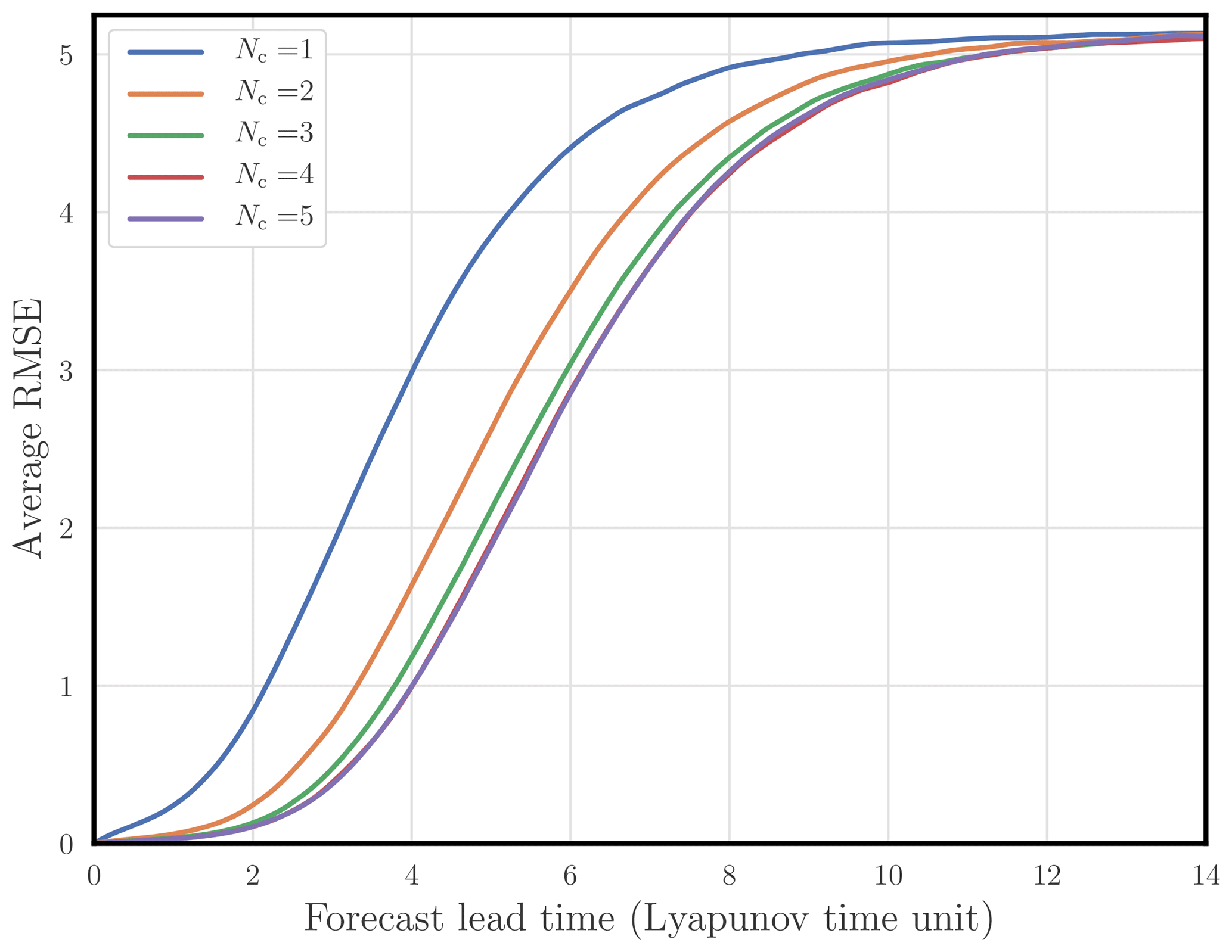
Figure 3 Average RMSE of the surrogate model (L96 with an RK2 structure) compared to the reference model (L96 with an RK4 integration scheme) as a function of the forecast lead time (in Lyapunov time unit) for an increasing number of compositions.
Figure 4 shows the trajectories of the reference and surrogate models starting from the same initial condition, as well as their difference, as a function of the forecast lead time. Their divergence becomes significant after 4 Lyapunov times and saturates after 8 Lyapunov times.
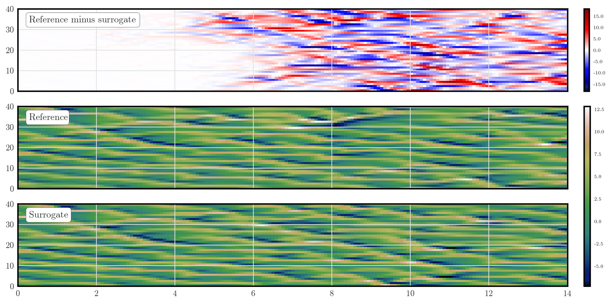
Figure 4 Density plot of the L96 reference and surrogate model trajectories, as well as their difference trajectory, as a function of the forecast lead time (in Lyapunov time unit). The observations are noiseless and dense; the model is not identifiable.
Next, the reference model trajectory is generated by the KS model (Nx=128) integrated with the ETDRK4 scheme, with Δt=0.05 and K=50 (this corresponds to about 0.25 Lyapunov time). We choose to implement the locality and homogeneity assumptions, with a stencil of width 9. The surrogate model is based on the RK4 scheme, with Nc=2 compositions. Note that in this experiment, the reference and surrogate models and their integration schemes significantly differ. We have Np=769 and Na=45. We choose and . The forecast time step δtf is somehow smaller than δta because the KS equations are stiff and so will the surrogate model be. This emphasises once again that we have learned about the intrinsic flow rate of the reference model and not a resolvent thereof. Alternatively, we could use a more robust integration scheme than RK4 such as ETDRK4 for the forecast.
Figure 5 shows the trajectories of the reference and surrogate models starting from the same initial condition, as well as their difference, as a function of the forecast lead time, for a stencil of 9. Their divergence becomes significant after 4 Lyapunov times and saturates after 8 Lyapunov times.
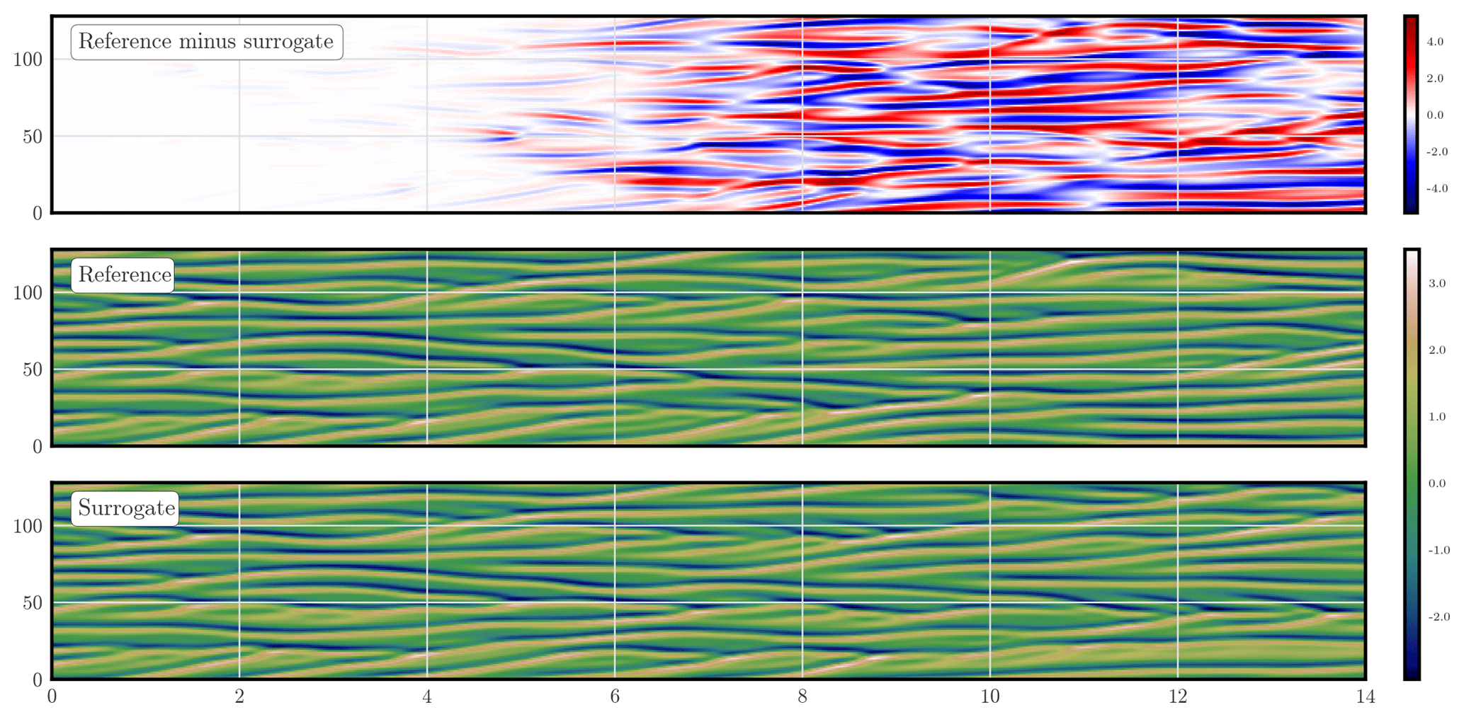
Figure 5 Density plot of the KS reference and surrogate model trajectories, as well as their difference trajectory, as a function of the forecast lead time (in Lyapunov time unit). The observations are noiseless and dense; the model is not identifiable.
To check whether the PDE of the KS model could be retrieved in spite of the differences in the method of integrations and representations, we have computed a Taylor expansion of all monomials in the surrogate ODE flow rate up to order 4 so as to obtain an approximately PDE equivalent. The coefficients of this PDE (up to order 4 in the expansion) are displayed in Fig. 6 and compared to the coefficients of the reference model's PDE. The match is good and the terms , , and are correctly identified as the dominant ones. Nonetheless, there are three non-negligible coefficients for higher-order terms that either might have been generated by the Taylor expansion or may originate from a degeneracy among the higher-order operators, or may simply be identified with a shortcoming of our specific ODE representation.

Figure 6 Coefficients of the surrogate PDE model (blue) resulting from the expansion of the surrogate ODEs and compared to the reference PDE's coefficients (orange).
4.4 Inferring the dynamics from partial and noisy observations
We come back to the L96 model, which is densely observed but with noisy observations that are generated using an independently identically distributed normal noise. The surrogate model is based on an RK4 scheme Nc=1 and a stencil of length 5, which makes the reference model identifiable. In this case, the outcome theoretically depends on the choice for rk and Qk, given that Eq. (17) is now used instead of Eq. (18). For the sake of simplicity, we have chosen them to be of the scalar forms and Qk≡qIx. In these synthetic experiments, σy is supposed to be known, while q is not. We only have a qualitative view of the potential mismatch between the reference and the surrogate model. Moreover, a Gaussian additive noise might not even be the best statistical model for such error. Nonetheless holding to the above Gaussian assumptions for model error, the optimal value of q could be determined using an empirical Bayes approach based on, for instance, the expectation–maximisation technique in order to determine the maximum a posteriori of the conditional density of q (see e.g. Dreano et al., 2017; Pulido et al., 2018). The use of advanced methods of that sort to estimate model error will be considered in future works, while, in the following, we have chosen values of q that yield near-to-optimal skill scores (typically ). Moreover, note that we have chosen the relatively small K=50. While we expect increasing K to be beneficial, especially with noisy observations, it would force us to address issues related to weak constraint 4D-Var optimisation for long time windows, a topic which is also beyond the scope of this paper. Preliminary results on this aspect are nonetheless discussed later in this section.
Figure 7 shows the forecast skill of the surrogate model as a function of the forecast lead time and for increasing noise in the observations.
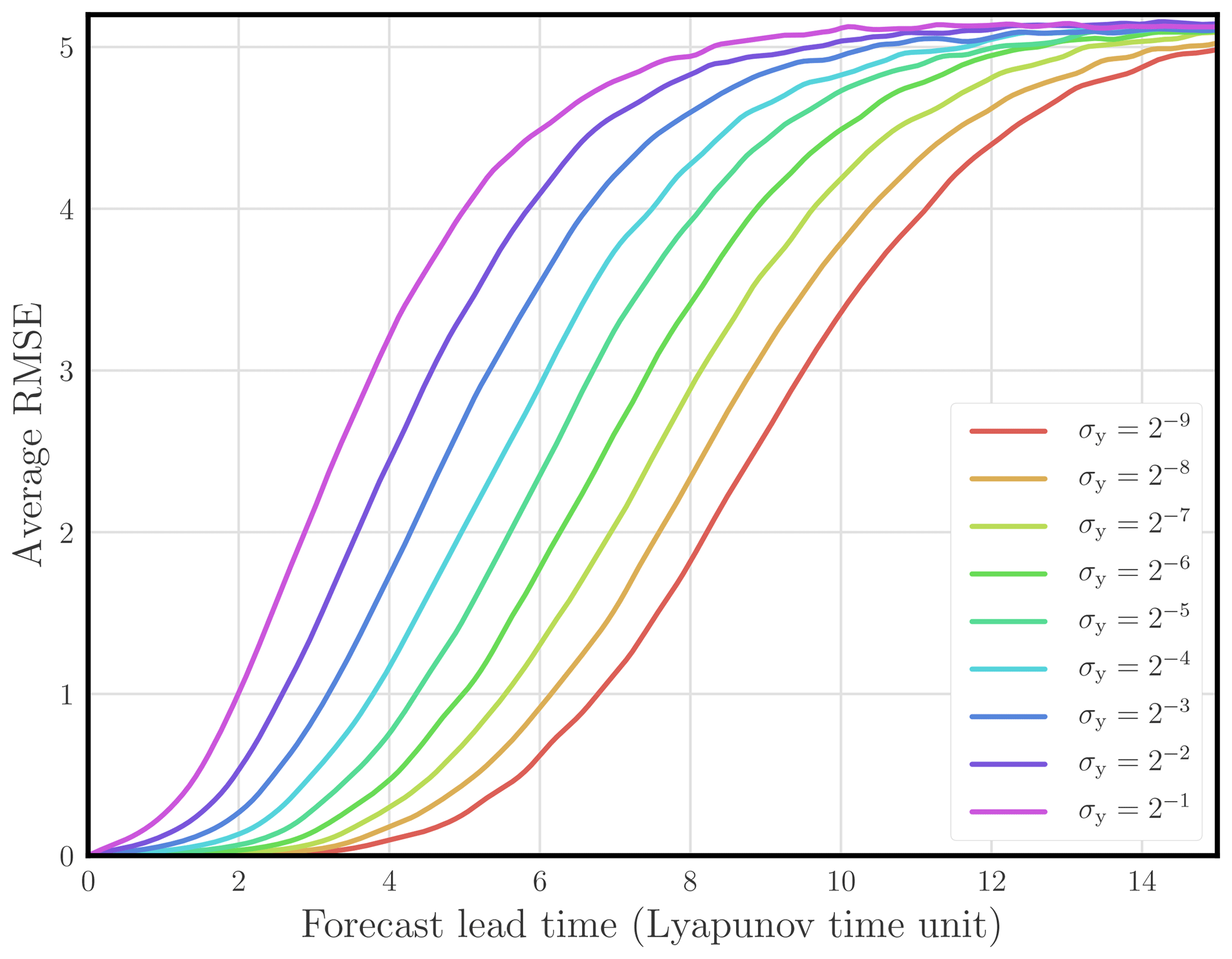
Figure 7 Average RMSE of the surrogate model (L96 with an RK4 structure) compared to the reference model (L96 with an RK4 integration scheme) as a function of the forecast lead time (in Lyapunov time unit) for a range of observation error standard deviations σy.
Even though, in this configuration, the model is identifiable, the reference value A0 for A may not correspond to a minimum of the cost function. The cost function might have several local minima. As a consequence, there is no guarantee, starting from a non-trivial initial value for A, that the model will be identified. Indeed, as seen in Fig. 7, the forecast skill degrades significantly as the observation error standard deviation is increased.
This is confirmed by Fig. 8, where the precisions in identifying the model, measured by either the spectral norm or the uniform norm , are plotted as functions of the observation error standard deviation.

Figure 8 Gap between the surrogate (L96 with an RK4 structure) and the (identifiable) reference dynamics (L96 with an RK4 integration scheme) as a function of the observation error standard deviation σy. Note the use of logarithmic scales.
Using the same setup, we have also reduced the number of observations. The observations of grid point values are regularly spaced and shifted by one grid cell at each observation time step. The initial A in the optimisation remains 0, while the initial state x0:K is taken as a cubic spline interpolation of the observations over the whole surrogate model grid.
If the observations are noiseless, the reference model is easily retrieved to a high precision down to a density of 1 site over 4. If the observations are noisy, the performance slowly degrades when the density is decreased down to about 1 site over 4, below which the minimisation, trapped in a deceiving local minimum, yields an improper surrogate model.
We would like to point out that in the case of noiseless observations, the performance depends little on the length of the training window, beyond a relatively short length, typically K=50. However, in the presence of noisy observations, the overall performance improves with longer K, as expected since the information content of the observations linearly increases with the length of the window.
Figure 9 displays the values of the coefficients in A with respect to the minimisation iteration index for the noiseless and fully observed case. As expected, 4 coefficients converge to the value specified by the exact L96 flow rate, while the 14 other coefficients collapse to 0.
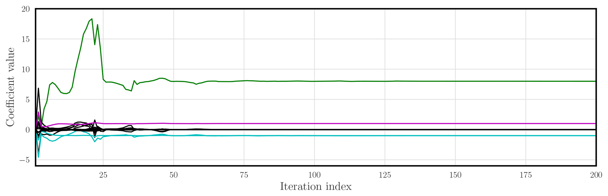
Figure 9 L96 is the reference model, which is fully observed without noise: plot of the Na=18 coefficients of the surrogate model as a function of the minimisation iteration number. The coefficient of the forcing (F) is in green, the coefficients of the convective terms are in cyan, and the dampening coefficient is in magenta.
Figure 10 shows the same but in the significantly noisy case where σy=1 and with a significantly longer window K=5000 (about 417 Lyapunov times).
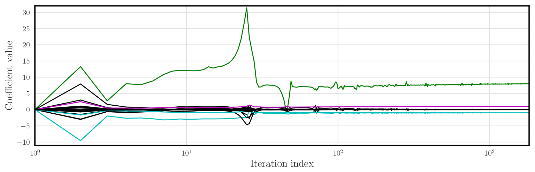
Figure 10 L96 is the reference model, which is fully observed with observation error standard deviation σy=1: plot of the Na=18 coefficients of the surrogate model as a function of the minimisation iteration number. Note that the index axis is in logarithmic scale. The coefficient of the forcing (F) is in green, the coefficients of the convective terms are in cyan, and the dampening coefficient is in magenta.

Figure 11 Density plot of the L05III reference and surrogate model trajectories, as well as their difference trajectory, as a function of the forecast lead time (in Lyapunov time unit). Panel (d) shows a zoom of the difference between times 4 and 5.
4.5 Inferring reduced dynamics of a multiscale model
In this experiment, we consider the L05III model. With the locality and the homogeneity assumptions, the scalability is typically linear with the size of the system, and we actually consider the 10-fold model where Nx=360 and Nu=3600 to demonstrate that no issues were encountered when scaling up the method. The large-scale variable x of the reference model is noiselessly and fully observed over a short training window (K=50, which corresponds to about 0.35 Lyapunov time), i.e. all slow variable values are observed, whereas the short-scale variable u is not observed. The surrogate model is based on the RK4 scheme and Nc=2 compositions. We choose to implement the locality and homogeneity assumptions, with a stencil of width 5. We have Np=161 and Na=18. We choose .
Figure 11 shows the trajectories of the reference and surrogate models starting from the same initial condition, as well as their difference, as a function of time.
The emergence of error, i.e. the divergence from the reference, appears as long darker stripes on the density plot of the difference (close to zero difference values appear as white or light colour). We argue that these stripes result from the emergence of sub-scale perturbations that are not properly represented by the surrogate model. Reciprocally there are long-lasting stripes of low error not yet impacted by sub-scale perturbations. As expected, and similarly to the L96 model, the perturbations are transported eastward, as shown by the upward tilt of the stripes in Fig. 11. Clearly, in this case, a flow rate of the form Eq. (2) could be insufficient. Adding a stochastic parametrisation with parameters additionally inferred might offer a solution, as in Pulido et al. (2018). Because of this mixed performance, the RMSE slowly degrades (compared to the other experiments reported so far) with the increase in the forecast lead time (not shown).
We have proposed to infer the dynamics of a reference model from its observation using Bayesian data assimilation, which is a new and original scope for data assimilation. Over a given training time window, the control variables are the state trajectory and the coefficients of an ODE representation for the surrogate model. We have chosen the surrogate model to be the composition of an explicit integration scheme (Runge–Kutta typically) applied to this ODE representation. Time invariance, space homogeneity, and locality of the dynamics can be enforced, making the method suitable for high-dimensional systems. The cost function of the data assimilation problem is minimised using the adjoint of the surrogate resolvent which is explicitly derived. Analogies between the surrogate resolvent and a deep neural network have been discussed as well as the impact of stability issues of the reference and surrogate dynamics.
The method has been applied to densely noiseless observed systems with identifiable reference models yielding a perfect reconstruction close to machine precision (L63 and L96 models). It has also been applied to densely or partially observed, identifiable or non-identifiable models with or without noise in the observations (L96 and KS models). For moderate noise and sufficiently dense observation, the method is successful in the sense that the forecast is accurate beyond several Lyapunov times. The method has also been used as a way to infer a reduced model for a multi-scale observed system (L05-III model). The reduced model was successful in emulating slow dynamics of the reference model, but could not properly account for the impact of the fast unresolved scale dynamics on the slow ones. A subgrid parametrisation would be required or would have to be inferred.
Two potential obstacles have been left aside on purpose but should later be addressed. First, the model error statistics have not been estimated. This could be achieved using for instance an empirical Bayesian analysis built on an ensemble-based stochastic expectation maximisation technique. This is an especially interesting problem since the potential discrepancy between the reference and the surrogate dynamics is in general non-trivial. Second, we have used relatively short training time windows. Numerical efficient training on longer windows will likely require use of advanced weak constraint variational optimisation techniques.
In this paper, only autonomous dynamics have been considered. We could at least partially extend the method to non-autonomous systems by keeping a static part for the pure dynamics and consider time-dependent forcing fields. We have not numerically explored non-homogeneous dynamics, but we have shown how to learn from them using non-homogeneous local representations.
A promising yet challenging path would be to consider implicit or semi-implicit schemes following for instance the idea in Chen et al. (2018). This idea is known in geophysical data assimilation as the continuous adjoint (see e.g. Bocquet, 2012). This would considerably strengthen the stability of the training and forecast steps at the cost of more intricate mathematical developments.
If observations keep coming after the training time window, then one can perform data assimilation using the ODE surrogate model of the reference model. This data assimilation scheme could only focus on state estimation or it could continue to update the ODE surrogate model for the forecast.
No datasets were used in this article.
In this Appendix, we show how to parametrise ϕA assuming locality of the representation, in the case where it is defined over a periodic one-dimensional domain, i.e. a circle. It is of the generic form
where π(n,p) is an integer such that . We can treat the bias, linear, and bilinear monomials separately into sectors, 0, 1, and 2, respectively. Let be the indices which span the columns of A for each of the three sectors i and the indices which span the entries of r for each of the three sectors i. Then, Eq. (A1) can be more explicitly written as
where the dummy index l for the linear terms browses the stencil, and the dummy indices l,m for the bilinear monomials browse the stencil, in the same way as we did in Sect. 2.2.1 to enumerate them. By enumeration, we find the following.
-
For the bias sector, we have p0(0)=0 and a0(0)=0.
-
For the linear sector, we have and , where [n] means the index in congruent to n modulo Nx, in order to respect the periodicity of the domain.
-
Finally, for the bilinear sector, we have and .
We observe that these indices , and do not depend on the site index n. They only indicate a relative position with respect to n. Hence, if homogeneity is additionally assumed, , and do not depend on n anymore and A becomes a vector.
B1 Differentiation of the RK schemes
It will be useful in the following to consider the variation of each ki, defined by Eq. (12b), with respect to either A or x:
where ϕA,i is ϕA evaluated at and is the tangent linear operator with respect to x of ϕA evaluated at . Equation (B1) can be written compactly in the form
where G is the matrix of size (NRKNx)×(NRKNx) defined by its Nx×Nx blocks , κ is the vector of size NRKNx which results from the stacking of the for , φ is the vector of size NRKNx which results from the stacking of the ϕA,i for , and is the identity matrix. The important point is that G is a lower triangular matrix and describes an iterative construction of the ki. Moreover, the diagonal entries of G are 1 by construction so that G is invertible and
This will be used to compute the variations of fA(x) via Eq. (12a).
B2 Integration step
We first consider the situation when the observation interval corresponds to one integration time step of the surrogate model, i.e. : with x≡xk. As a result, the time index k can be omitted here. We will later consider the composition of several integration schemes (Nc≥2). Equation (12a) is written again but as
where is the matrix of a size Nx×(NRKNx) tensor product of the vector β defined by , i.e. the coefficients of the RK scheme as defined in Eq. (12a), with the state space identity matrix, and where κ is the vector of size NRKNx defined after Eq. (B2). Looking first at the gradient with respect to the state variable, and using Eq. (B3), we have
which yields the adjoint operator
Let us consider an arbitrary vector ; we have
To avoid computing G−T explicitly, let us define the vector such that
Because GT is upper triangular with diagonal entries of value 1, z is the solution of a linear system easily solvable iteratively, which stands as an adjoint/dual to the RK iterative construction. Hence, we finally obtain a formula and algorithm to evaluate
which is key to computing Eq. (19). Indeed, Eq. (19) now reads as
where zk is the iterative solution of the system for .
Second, let us look at the gradient of with respect to A. From Eqs. (B4) and (B3), and now considering variations with respect to A, we obtain
which yields, using z as defined by Eq. (B8),
For each , let us introduce , and let us denote the subvector of z for the ith block of the Runge–Kutta scheme. Then we have, for and ,
This is key to efficiently computing Eq. (20), which now reads as
where zk is the solution of . The index k of Gk indicates that the operators defined in the entries of G are evaluated at xk.
B3 Composition of integration steps
We now consider a resolvent which is the composition of integration steps over : , where x is an alias to xk. Let us first look at the gradient with respect to the state variable. Within the scope of this section, we define x0≡x and for : . Hence, . We also define as the tangent linear operator of fA at xl. By the Leibniz rule, we obtain
We can now apply Eq. (B9) to each individual integration step and obtain for any
where zl is the solution of
Hence, to compute , we define and for : . This finally reads as
for , where zl is the solution of
To compute the key terms in the gradients Eq. (19), d must be chosen to be where and
Second, we look at the gradient with respect to A. In this case, the application of the Leibniz rule yields
where . But ∇AfA(xl), which focuses on a single integration step, is given by Eq. (B11),
and from Eq. (B12),
As a result, we obtain
where zk,l is the solution of
All of these results, Eqs. (B10), (B14), (B20), and (B24), allow us to efficiently compute the gradients of the cost function with respect to both A and x0:K. Note, however, that they have been derived under the simplifying assumption that ϕA is given by Eq. (2) with a traditional matrix multiplication between A and r(x), but not by the compact Eq. (8). When relying on homogeneity and/or locality, the calculation of the gradient with respect to A follows the principle described above but requires further adaptations, which can be derived using Eq. (A2), with the asset of strongly reducing the computational burden.
As an alternative to the explicit computation of the gradients of Eq. (17) and the associated adjoint models, we have used PyTorch and TensorFlow as automatic differentiation tools. Only the cost function code needs to be implemented. We made a few tests of the experiments of Sect. 4 that showed that the fastest code is a C++ implementation using the explicit gradients, followed by an implementation using Python/Numpy/Numba using the explicit gradients, followed
by a much slower implementation with TensorFlow (graph execution), followed by an implementation with TensorFlow (eager execution) and finally with PyTorch. Our experiments made use of a multi-core CPU and/or a GPU. This purely qualitative ranking is not surprising
since (i) PyTorch and TensorFlow excel in tensor algebra operations which are not massively used in the way we built our cost function with relatively few but significant parameters, and (ii) the time spent in the development of each approach scales with their speed.
MB first developed the theory, implemented, ran, and interpreted the numerical experiments, and wrote the original version of the manuscript. All authors discussed the theory, interpreted the results, and edited the manuscript. The four authors approved the manuscript for publication.
The authors declare that they have no conflict of interest.
The authors are grateful to two anonymous reviewers and Olivier Talagrand acting as editor for their comments and suggestions. Marc Bocquet is thankful to Said Ouala and Ronan Fablet for enlightening discussions. CEREA and LOCEAN are members of the Institut Pierre-Simon Laplace (IPSL).
This research has been supported by the Norwegian Research Council (project REDDA (grant no. 250711)).
This paper was edited by Olivier Talagrand and reviewed by two anonymous referees.
Abarbanel, H. D. I., Rozdeba, P. J., and Shirman, S.: Machine Learning: Deepest Learning as Statistical Data Assimilation Problems, Neural Comput., 30, 2025–2055, https://doi.org/10.1162/neco_a_01094, 2018. a, b
Amezcua, J., Goodliff, M., and van Leeuwen, P.-J.: A weak-constraint 4DEnsembleVar. Part I: formulation and simple model experiments, Tellus A, 69, 1271564, https://doi.org/10.1080/16000870.2016.1271564, 2017. a
Asch, M., Bocquet, M., and Nodet, M.: Data Assimilation: Methods, Algorithms, and Applications, Fundamentals of Algorithms, SIAM, Philadelphia, 2016. a, b
Aster, R. C., Borchers, B., and Thuber, C. H.: Parameter Estimation and Inverse Problems, Elsevier Academic Press, 2nd Edn., 2013. a
Bocquet, M.: Parameter field estimation for atmospheric dispersion: Application to the Chernobyl accident using 4D-Var, Q. J. Roy. Meteor. Soc., 138, 664–681, https://doi.org/10.1002/qj.961, 2012. a, b
Brunton, S. L., Proctor, J. L., and Kutz, J. N.: Discovering governing equations from data by sparse identification of nonlinear dynamical systems, P. Natl. Acad. Sci. USA, 113, 3932–3937, https://doi.org/10.1073/pnas.1517384113, 2016. a, b
Buizza, R., Miller, M., and Palmer, T. N.: Stochastic representation of model uncertainties in the ECMWF ensemble prediction system, Q. J. Roy. Meteor. Soc., 125, 2887–2908, 1999. a
Byrd, R. H., Lu, P., and Nocedal, J.: A Limited Memory Algorithm for Bound Constrained Optimization, SIAM J. Sci. Stat. Comp., 16, 1190–1208, 1995. a
Carlu, M., Ginelli, F., Lucarini, V., and Politi, A.: Lyapunov analysis of multiscale dynamics: the slow bundle of the two-scale Lorenz 96 model, Nonlin. Processes Geophys., 26, 73–89, https://doi.org/10.5194/npg-26-73-2019, 2019. a
Carrassi, A. and Vannitsem, S.: Accounting for model error in variational data assimilation: A deterministic formulation, Mon. Weather Rev., 138, 3369–3386, https://doi.org/10.1175/2010MWR3192.1, 2010. a
Carrassi, A., Bocquet, M., Bertino, L., and Evensen, G.: Data Assimilation in the Geosciences: An overview on methods, issues, and perspectives, WIREs Climate Change, 9, e535, https://doi.org/10.1002/wcc.535, 2018. a
Chang, B., Meng, L., Haber, E., Tung, F., and Begert, D.: Multi-level residual networks from dynamical systems view, in: Proceedings of ICLR 2018, 2018. a
Chen, T. Q., Rubanova, Y., Bettencourt, J., and Duvenaud, D.: Neural ordinary differential equations, in: Advances in Neural Information Processing Systems, 6571–6583, 2018. a
Dreano, D., Tandeo, P., Pulido, M., Ait-El-Fquih, B., Chonavel, T., and Hoteit, I.: Estimating model error covariances in nonlinear state-space models using Kalman smoothing and the expectation-maximisation algorithm, Q. J. Roy. Meteor. Soc., 143, 1877–1885, https://doi.org/10.1002/qj.3048, 2017. a
Dueben, P. D. and Bauer, P.: Challenges and design choices for global weather and climate models based on machine learning, Geosci. Model Dev., 11, 3999–4009, https://doi.org/10.5194/gmd-11-3999-2018, 2018. a
Fablet, R., Ouala, S., and Herzet, C.: Bilinear residual neural network for the identification and forecasting of dynamical systems, in: EUSIPCO 2018, European Signal Processing Conference, Rome, Italy, 1–5, available at: https://hal.archives-ouvertes.fr/hal-01686766 (last access: 8 July 2019), 2018. a, b, c, d
Gautschi, W.: Numerical analysis, Springer Science & Business Media, 2nd Edn., 2012. a
Goodfellow, I., Bengio, Y., and Courville, A.: Deep learning, The MIT Press, Cambridge Massachusetts, London, England, 2016. a
Grudzien, C., Carrassi, A., and Bocquet, M.: Chaotic dynamics and the role of covariance inflation for reduced rank Kalman filters with model error, Nonlin. Processes Geophys., 25, 633–648, https://doi.org/10.5194/npg-25-633-2018, 2018. a
Harlim, J.: Model error in data assimilation, in: Nonlinear and stochastic climate dynamics, edited by: Franzke, C. L. E. and O'Kane, T. J., Cambridge University Press, 276–317, https://doi.org/10.1017/9781316339251.011, 2017. a
Harlim, J.: Data-driven computational methods: parameter and operator estimations, Cambridge University Press, Cambridge, 2018. a
Hodyss, D.: Ensemble State Estimation for Nonlinear Systems Using Polynomial Expansions in the Innovation, Mon. Weather Rev., 139, 3571–3588, https://doi.org/10.1175/2011MWR3558.1, 2011. a
Hodyss, D.: Accounting for Skewness in Ensemble Data Assimilation, Mon. Weather Rev., 140, 2346–2358, https://doi.org/10.1175/MWR-D-11-00198.1, 2012. a
Hsieh, W. W. and Tang, B.: Applying Neural Network Models to Prediction and Data Analysis in Meteorology and Oceanography, B. Am. Meteorol. Soc., 79, 1855–1870, https://doi.org/10.1175/1520-0477(1998)079<1855:ANNMTP>2.0.CO;2, 1998. a
Janjić, T., Bormann, N., Bocquet, M., Carton, J. A., Cohn, S. E., Dance, S. L., Losa, S. N., Nichols, N. K., Potthast, R., Waller, J. A., and Weston, P.: On the representation error in data assimilation, Q. J. Roy. Meteor. Soc., 144, 1257–1278, https://doi.org/10.1002/qj.3130, 2018. a
Kalnay, E.: Atmospheric Modeling, Data Assimilation and Predictability, Cambridge University Press, Cambridge, 2002. a
Kassam, A.-K. and Trefethen, L. N.: Fourth-Order Time-Stepping For Stiff PDEs, Siam J. Sci. Comput., 26, 1214–1233, https://doi.org/10.1137/S1064827502410633, 2005. a
Kondrashov, D. and Chrekroun, M. D.: Data-adaptive harmonic spectra and multilayer Stuart-Landau models, Chaos, 27, 093110, https://doi.org/10.1016/j.physd.2014.12.005, 2017. a
Kondrashov, D., Chrekroun, M. D., and Ghil, M.: Data-driven non-Markovian closure models, Physica D, 297, 33–55, https://doi.org/10.1063/1.4989400, 2015. a
Kondrashov, D., Chrekroun, M. D., Yuan, X., and Ghil, M.: Data-adaptive harmonic decomposition and stochastic modeling of Arctic sea ice, in: Advances in Nonlinear Geosciences, edited by: Tsonis, A., Springer, Cham, 179–205, https://doi.org/10.1007/978-3-319-58895-7_10, 2018. a
Kuramoto, Y. and Tsuzuki, T.: Persistent propagation of concentration waves in dissipative media far from thermal equilibrium, Prog. Theor. Phys., 55, 356–369, 1976. a
Lguensat, R., Tandeo, P., Ailliot, P., Pulido, M., and Fablet, R.: The Analog Data Assimilation, Mon. Weather Rev., 145, 4093–4107, https://doi.org/10.1175/MWR-D-16-0441.1, 2017. a
Long, Z., Lu, Y., Ma, X., and Dong, B.: PDE-Net: Learning PDEs from Data, in: Proceedings of the 35th International Conference on Machine Learning, 2018. a
Lorenz, E. N.: Deterministic nonperiodic flow, J. Atmos. Sci., 20, 130–141, 1963. a
Lorenz, E. N.: Designing Chaotic Models, J. Atmos. Sci., 62, 1574–1587, https://doi.org/10.1175/JAS3430.1, 2005. a
Lorenz, E. N. and Emanuel, K. A.: Optimal sites for supplementary weather observations: simulation with a small model, J. Atmos. Sci., 55, 399–414, https://doi.org/10.1175/1520-0469(1998)055<0399:OSFSWO>2.0.CO;2, 1998. a
Magnusson, L. and Källén, E.: Factors influencing skill improvements in the ECMWF forecasting system, Mon. Weather Rev., 141, 3142–3153, https://doi.org/10.1175/MWR-D-12-00318.1, 2013. a
Mitchell, L. and Carrassi, A.: Accounting for model error due to unresolved scales within ensemble Kalman filtering, Q. J. Roy. Meteor. Soc., 141, 1417–1428, https://doi.org/10.1175/MWR-D-16-0478.1, 2015. a
Paduart, J., Lauwers, L., Swevers, J., Smolders, K., Schoukens, J., and Pintelon, R.: Identification of nonlinear systems using polynomial nonlinear state space models, Automatica, 46, 647–656, https://doi.org/10.1016/j.automatica.2010.01.001, 2010. a, b
Park, D. C. and Zhu, Y.: Bilinear recurrent neural network, IEEE World Congress on Computational Intelligence, Neural Networks, 3, 1459–1464, 1994. a
Pathak, J., Lu, Z., Hunt, B. R., Girvan, M., and Ott, E.: Using machine learning to replicate chaotic attractors and calculate Lyapunov exponents from data, Chaos, 27, 121102, https://doi.org/10.1063/1.5010300, 2017. a
Pathak, J., Hunt, B., Girvan, M., Lu, Z., and Ott, E.: Model-Free Prediction of Large Spatiotemporally Chaotic Systems from Data: A Reservoir Computing Approach, Phys. Rev. Lett., 120, 024102, https://doi.org/10.1103/PhysRevLett.120.024102, 2018. a
Pulido, M., Tandeo, P., Bocquet, M., Carrassi, A., and Lucini, M.: Stochastic parameterization identification using ensemble Kalman filtering combined with maximum likelihood methods, Tellus A, 70, 1442099, https://doi.org/10.1080/16000870.2018.1442099, 2018. a, b, c, d, e
Raanes, P. N., Carrassi, A., and Bertino, L.: Extending the square root method to account for additive forecast noise in ensemble methods, Mon. Weather Rev., 143, 3857–3873, https://doi.org/10.1175/MWR-D-14-00375.1, 2015. a
Raanes, P. N., Bocquet, M., and Carrassi, A.: Adaptive covariance inflation in the ensemble Kalman filter by Gaussian scale mixtures, Q. J. Roy. Meteor. Soc., 145, 53–75, https://doi.org/10.1002/qj.3386, 2019. a
Resseguier, V., Mémin, E., and Chapron, B.: Geophysical flows under location uncertainty, Part I Random transport and general models, Geophys. Astro. Fluid, 111, 149–176, https://doi.org/10.1080/03091929.2017.1310210, 2017. a
Ruiz, J. J., Pulido, M., and Miyoshi, T.: Estimating model parameters with ensemble-based data assimilation: A Review, J. Meteorol. Soc. Jpn., 91, 79–99, https://doi.org/10.2151/jmsj.2013-201, 2013. a
Sakov, P., Haussaire, J.-M., and Bocquet, M.: An iterative ensemble Kalman filter in presence of additive model error, Q. J. Roy. Meteor. Soc., 144, 1297–1309, https://doi.org/10.1002/qj.3213, 2018. a
Sivashinsky, G. I.: Nonlinear analysis of hydrodynamic instability in laminar flames-I. Derivation of basic equations, Acta Astronaut., 4, 1177–1206, 1977. a
Tandeo, P., Ailliot, P., Bocquet, M., Carrassi, A., Miyoshi, T., Pulido, M., and Zhen, Y.: Joint Estimation of Model and Observation Error Covariance Matrices in Data Assimilation: a Review, available at: https://hal-imt-atlantique.archives-ouvertes.fr/hal-01867958 (last access: 8 July 2019), submitted, 2019. a
Trémolet, Y.: Accounting for an imperfect model in 4D-Var, Q. J. Roy. Meteor. Soc., 132, 2483–2504, 2006. a
Wang, Y.-J. and Lin, C.-T.: Runge-Kutta neural network for identification of dynamical systems in high accuracy, IEEE T. Neural Networ., 9, 294–307, https://doi.org/10.1109/72.661124, 1998. a, b
Weinan, E.: A proposal on machine learning via dynamical systems, Commun. Math. Stat., 5, 1–11, https://doi.org/10.1007/s40304-017-0103-z, 2017. a
Whitaker, J. S. and Hamill, T. M.: Evaluating Methods to Account for System Errors in Ensemble Data Assimilation, Mon. Weather Rev., 140, 3078–3089, https://doi.org/10.1175/MWR-D-11-00276.1, 2012. a
The Lyapunov time is defined as the inverse of the first Lyapunov exponent, i.e. the typical time over which the error grows by a factor e.
We choose the qualifier densely observed instead of fully observed because there is no way to tell from the observations alone whether the reference model is fully observed.
- Abstract
- Introduction
- Model identification as a data assimilation problem
- Discussion of the theoretical points
- Numerical illustrations
- Conclusions
- Data availability
- Appendix A: Parametrisation of ϕA for local representations defined over a circle
- Appendix B: Computations of the gradients with respect to A and x0:K
- Appendix C: Adjoint differentiation with PyTorch and TensorFlow
- Author contributions
- Competing interests
- Acknowledgements
- Financial support
- Review statement
- References