Connection between encounter volume and diffusivity in geophysical flows

Trajectory encounter volume – the volume of fluid that passes close to a reference fluid parcel over some time interval – has been recently introduced as a measure of mixing potential of a flow. Diffusivity is the most commonly used characteristic of turbulent diffusion. We derive the analytical relationship between the encounter volume and diffusivity under the assumption of an isotropic random walk, i.e., diffusive motion, in one and two dimensions. We apply the derived formulas to produce maps of encounter volume and the corresponding diffusivity in the Gulf Stream region of the North Atlantic based on satellite altimetry, and discuss the mixing properties of Gulf Stream rings. Advantages offered by the derived formula for estimating diffusivity from oceanographic data are discussed, as well as applications to other disciplines.

1 Introduction

The frequency of close encounters between different objects or organisms can be a fundamental metric in social and mechanical systems. The chances that a person will meet a new friend or contract a new disease during the course of a day is influenced by the number of distinct individuals that he or she comes into close contact with. The chances that a predator will ingest a poisonous prey, or that a mushroom hunter will mistakenly pick up a poisonous variety, is influenced by the number of distinct species or variety of prey or mushrooms that are encountered. In fluid systems, the exchange of properties such as temperature, salinity or humidity between a given fluid element and its surroundings is influenced by the number of other distinct fluid elements that pass close by over a given time period. In all these cases it is best to think of close encounters as providing the potential, if not necessarily the act, of transmission of germs, toxins, heat, salinity, etc.

In cases of property exchange within continuous media such as air or water, it may be most meaningful to talk about a mass or volume passing within some radius of a reference fluid element as this element moves along its trajectory. Rypina and Pratt (2017) introduce a trajectory encounter volume, V, the volume of fluid that comes in contact with the reference fluid parcel over a finite time interval. The increase in V over time is one measure of the mixing potential of the element, “mixing” being the irreversible exchange of properties between different water parcels. Thus, fluid parcels that have large encounter volumes as they move through the flow field have large mixing potential, i.e., an opportunity to exchange properties with other fluid parcels, and vice versa.

In order to formally define the encounter volume V, Rypina and Pratt (2017) subdivide the entire fluid into infinitesimal fluid elements with volumes dV_i, and define the encounter volume for each fluid element to be the total volume of fluid that passes within a radius R of it over a finite time interval $t_{\mathrm{0}}<t<t_{\mathrm{0}}+T$, i.e.,

$$\begin{array}{}\text{(1)}& V\left({\mathit{x}}_{\mathrm{0}};t_{\mathrm{0}},T,R\right)=\underset{\mathrm{d}{V}_i\to \mathrm{0}}{lim}{\mathrm{\Sigma }}_i\mathrm{d}{V}_i.\end{array}$$

In practice, for dense uniform grids of trajectories, ${\mathit{x}}_{\mathit{k}}\left({\mathit{x}}_{\mathrm{0}k};t_{\mathrm{0}},T\right),k=\mathrm{1},\mathrm{\dots },K$, where t₀ is the starting time, T is the trajectory integration time, and x_0k is the trajectory initial position satisfying $\mathit{x}\left({\mathit{x}}_{\mathrm{0}};t_{\mathrm{0}},T=\mathrm{0}\right)={\mathit{x}}_{\mathrm{0}}$, both the limit and the subscript in the above definition Eq. (1) can be dropped. In this case, the encounter volume can be approximated by

$$\begin{array}{}\text{(2)}& V\approx N\mathit{\delta }V,\end{array}$$

where the encounter number,

$$\begin{array}{ll}{\displaystyle }& {\displaystyle }N\left({\mathit{x}}_{\mathrm{0}\mathrm{ref}};t_{\mathrm{0}},T,R\right)=\sum _{\begin{array}{l}k=\mathrm{1}\\ k\ne \mathrm{ref}\end{array}}^K\\ \text{(3)}& {\displaystyle }& {\displaystyle }I\left(min\left(\left|{\mathit{x}}_{\mathit{k}}\left({\mathit{x}}_{\mathrm{0}k};t_{\mathrm{0}},T\right)-{\mathit{x}}_{\mathrm{ref}}\left({\mathit{x}}_{\mathrm{0}\mathrm{ref}};t_{\mathrm{0}},T\right)\right|\right)\le R\right),\end{array}$$

is the number of trajectories that come within a radius R of the reference trajectory, ${\mathit{x}}_{\mathrm{ref}}\left({\mathit{x}}_{\mathrm{0}\mathrm{ref}};t_{\mathrm{0}},T\right)$, over a time $t_{\mathrm{0}}<t<t_{\mathrm{0}}+T$. Here the indicator function I is 1 if true and 0 if false, and K is the total number of particles. As in Rypina and Pratt (2017), we define encounter volume based on the number of encounters with different trajectories, not the total number of encounter events (see the schematic diagram of trajectory encounters in Fig. 1). Rypina and Pratt (2017) discuss how the encounter volume can be used to identify Lagrangian coherent structures (LCS) such as stable and unstable manifolds of hyperbolic trajectories and regions foliated by the KAM-like tori surrounding elliptic trajectories in realistic geophysical flows. A detailed comparison between the encounter volume method and some other Lagrangian methods of LCS identification, as well as the dependences on parameters, $t_{\mathrm{0}},T,R$, and on grid spacing (or on the number of trajectories, K), and the relative advantages of different techniques, was given in Rypina and Pratt (2017). The interested reader is referred to that earlier paper for details. The current paper is concerned only with the question of finding the connection between the encounter volume and diffusivity, rather than identifying LCS.

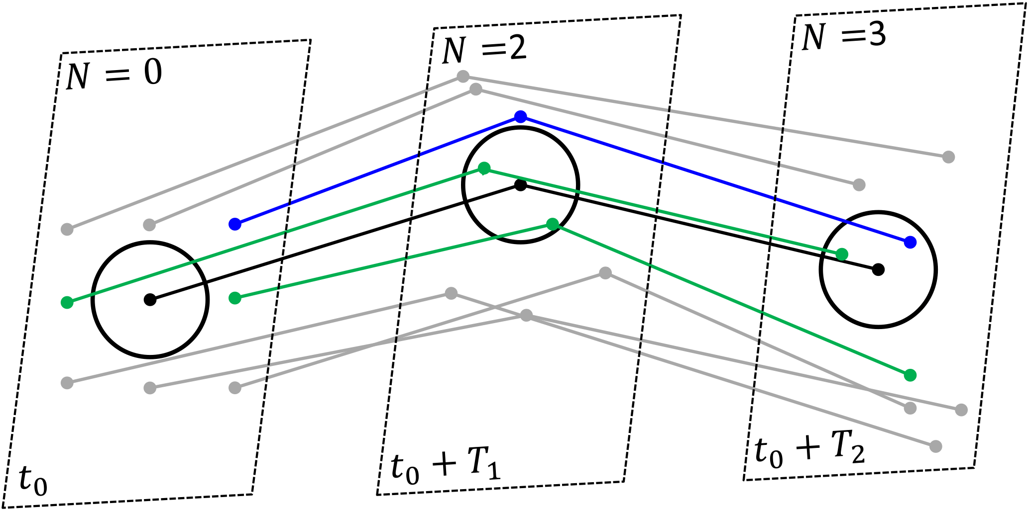
Figure 1 Schematic diagram of trajectory encounters, showing trajectories of nine particles, with dots indicating positions of particles at three time instances, at the release time, t₀, and at two later times, t₀+T₁ and t₀+T₂. The reference trajectory and the encounter sphere are shown in black, trajectories that do not encounter the reference trajectory are in grey, and trajectories that encounter the reference trajectory are in green if encounters occur at t₀+T₁, and in blue if encounters occur at t₀+T₂. Time slices are schematically shown by dashed rectangles, and the encounter number, N, is indicated at the top of each time slice.

Given the seemingly fundamental importance of close encounters, it is of interest to relate metrics such as V to other bulk measures of interactions within the system. For example, in some cases it may be more feasible to count encounters rather than to measure interactions or property exchanges directly, whereas in other cases the number of encounters might be most pertinent to the process in question but difficult to measure directly. In many applications, including ocean turbulence, the most commonly used metric of mixing is the eddy diffusivity, κ, a quantity that relates transport of fluid elements by turbulent eddies to diffusion (LaCasce, 2008; Vallis, 2006; Rypina et al., 2012; Kamenkovich et al., 2015). The underlying assumption is that the eddy field drives downgradient tracer transfer, similar to molecular diffusion but with a different (larger) diffusion coefficient. This diffusive parameterization of eddies has been implemented in many non-eddy-resolving oceanic numerical models. The diffusivity can be measured by a variety of means, including dye release (Ledwell et al., 2000; Sundermeyer and Ledwell, 2001; Rypina et al., 2016), surface drifter dispersion (Okubo, 1971; Davis, 1991; LaCasce, 2008; La Casce et al., 2014; Rypina et al., 2012, 2016), and property budgets (Munk, 1966). In numerical models κ is often assumed constant in both time and space, or related in some simplified manner to the large-scale flow properties (Visbeck et al., 1997).

Because the purpose of the diffusivity coefficient κ is to quantify the intensity of the eddy-induced tracer transfer, i.e., the intensity of mixing, it is tempting to relate it to the encounter volume, V, which quantifies the mixing potential of a flow and thus is closely related to tracer mixing. Such an analytical connection between the encounter volume and diffusivity could potentially also be useful for the parameterizations of eddy effects in numerical models. The main goal of this paper is to develop a relationship between V and κ in one and two dimensions. Specifically, we seek an analytical expression for the encounter volume, V, i.e., the volume of fluid that passed within radius R from a reference particle over time, as a function of κ. The relationship is not as straightforward as one might first imagine, but can nevertheless be written down straightforwardly in the long-time limit. This is opportune, since the concept of eddy diffusivity is most relevant in the long-time limit.

2 Connection between encounter volume and diffusivity

This problem was framed in mathematical terms in Rypina and Pratt (2017), who outlined some initial steps towards deriving the analytical connection between encounter volume and diffusivity but did not finish the derivation. In this section, we complete the derivation.

2.1 Main idea for the derivation

Let us start by considering the simplest diffusive random walk process in one or two dimensions, where particles take steps of fixed length Δx in random directions along the x-axis in 1-D or along both the x- and y-axes in 2-D, respectively, at fixed time intervals Δt.

The single particle dispersion, i.e., the ensemble-averaged square displacement from the particle's initial position, is $D_{\text{1-D}}=\langle {\left(x-x_{\mathrm{0}}\right)}^{\mathrm{2}}\rangle$ and $D_{\text{2-D}}=\langle {\left(x-x_{\mathrm{0}}\right)}^{\mathrm{2}}+{\left(y-y_{\mathrm{0}}\right)}^{\mathrm{2}}\rangle$ in 1-D or 2-D, respectively. For a diffusive process, the dispersion grows linearly with time, and the constant proportionality coefficient is related to diffusivity. Specifically, D_1-D=2κ_1-Dt with ${\mathit{\kappa }}_{\text{1-D}}=\mathrm{\Delta }{x}^{\mathrm{2}}/\left(\mathrm{2}\mathrm{\Delta }t\right)$, and D_2-D=4K_2-Dt with ${\mathit{\kappa }}_{\text{2-D}}=\mathrm{\Delta }{x}^{\mathrm{2}}/\left(\mathrm{4}\mathrm{\Delta }t\right)$.

It is convenient to consider the motion in a reference frame that is moving with the reference particle. In that reference frame, the reference particle will always stay at the origin, while other particles will still be involved in a random walk motion, but with a diffusivity twice that in the stationary frame, κ^moving=2κ^stationary (Rypina and Pratt, 2017).

The problem of finding the encounter number is then reduced to counting the number of randomly walking particles (with diffusivity κ^moving) that come within radius R of the origin in the moving frame. This is related to a classic problem in statistics – the problem of a random walker reaching an absorbing boundary, usually referred to as “a cliff” (because once a walker reaches the absorbing boundary, it falls off the cliff), over a time interval from 0 to t.

In the next section we will provide formal solutions; here we simply outline the steps to streamline the derivation. We start by deriving the appropriate diffusion equation for the probability density function, p(x,t), of random walkers in 1-D or 2-D:

$$\begin{array}{}\text{(4)}& {\displaystyle \frac{\partial p}{\partial t}}=\mathit{\kappa }{\mathrm{\nabla }}^{\mathrm{2}}p.\end{array}$$

We place a cliff, x_c, at the perimeter of the encounter sphere, i.e., at a distance R from the origin, and impose an absorbing boundary condition at a cliff,

$$\begin{array}{}\text{(5a)}& p({\mathit{x}}_{\mathrm{c}},t)=\mathrm{0},\end{array}$$

which removes (or “absorbs”) particles that have reached the cliff (see Fig. 2 for a schematic diagram). We then consider a random walker that is initially located at a point x₀ outside the cliff at t=0, i.e.,

$$\begin{array}{}\text{(5b)}& p\left(\mathit{x},t=\mathrm{0}\right)=\mathit{\delta }\left(\mathit{x}-{\mathit{x}}_{\mathrm{0}}\right),\end{array}$$

and we write an analytical solution for the probability density function satisfying Eqs. (4)–(5),

$$\begin{array}{}\text{(6)}& G\left(\mathit{x},t;{\mathit{x}}_{\mathrm{0}},{\mathit{x}}_{\mathrm{c}}\right),\end{array}$$

that quantifies the probability of finding a random walker initially located at x₀ at any location x outside of the cliff at a later time t>0. In mathematical terms, G is Green's function of the diffusion equation.

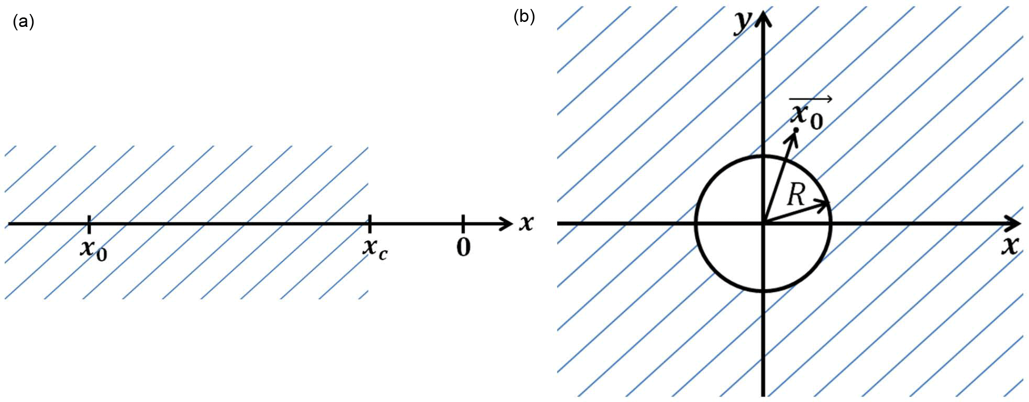
Figure 2 Schematic diagram in 1-D (a) and 2-D (b). Hatched areas show semi-infinite domains outside of the cliff.

The survival probability, which quantifies the probability that a random walker initially located at x₀ at t=0 has “survived” over time t without falling off the cliff, is

$$\begin{array}{}\text{(7)}& S\left(t;{\mathit{x}}_{\mathrm{0}},{\mathit{x}}_{\mathrm{c}}\right)=\int G\left(\mathit{x},t;{\mathit{x}}_{\mathrm{0}},{\mathit{x}}_{\mathrm{c}}\right)\mathrm{d}\mathit{x}\end{array}$$

where the integral is taken over all locations outside of the cliff. The encounter, or “non-survival”, probability can then be written as the conjugate quantity,

$$\begin{array}{}\text{(8)}& P_{\mathrm{en}}\left(t;{\mathit{x}}_{\mathrm{0}},{\mathit{x}}_{\mathrm{c}}\right)=\mathrm{1}-S\left(t;{\mathit{x}}_{\mathrm{0}},{\mathit{x}}_{\mathrm{c}}\right),\end{array}$$

which quantifies the probability that a random walker initially located at x₀ at t=0 has reached, or fallen off, the cliff over time t. This allows one to write the encounter volume, i.e., the volume occupied by particles that were initially located outside of the cliff and that have reached the cliff by time t, as

$$\begin{array}{}\text{(9)}& V\left(t;{\mathit{x}}_{\mathrm{c}}\right)=\int P_{\mathrm{en}}\left(t;{\mathit{x}}_{\mathrm{0}},{\mathit{x}}_{\mathrm{c}}\right)\mathrm{d}{\mathit{x}}_{\mathrm{0}}\end{array}$$

where the integral is taken over all initial positions outside of the cliff.

2.2 1-D case

Consider a random walker initially located at the origin, who takes, with a probability of 1∕2, a fixed step Δx to the right or to the left along the x-axis after each time interval Δt. Then the probability of finding a walker at a location x=nΔx after (m+1) steps is

$$\begin{array}{ll}{\displaystyle }& {\displaystyle }p\left(n\mathrm{\Delta }x,\left(m+\mathrm{1}\right)\mathrm{\Delta }t\right)=\mathrm{1}/\mathrm{2}[p\left(\left(n-\mathrm{1}\right)\mathrm{\Delta }x,m\mathrm{\Delta }t\right)\\ \text{(10)}& {\displaystyle }& {\displaystyle }+p\left(\left(n+\mathrm{1}\right)\mathrm{\Delta }x,m\mathrm{\Delta }t\right)].\end{array}$$

Using a Taylor series expansion in Δx and Δt, we can write down the finite-difference approximation to the above expression as

$$\begin{array}{ll}{\displaystyle }p\left(x,t\right)& {\displaystyle }+\mathrm{\Delta }t{\displaystyle \frac{\partial p}{\partial t}}={\displaystyle \frac{\mathrm{1}}{\mathrm{2}}}\left[p\left(x,t\right)-\mathrm{\Delta }x{\displaystyle \frac{\partial p}{\partial x}}+{\displaystyle \frac{\mathrm{\Delta }{x}^{\mathrm{2}}}{\mathrm{2}}}{\displaystyle \frac{{\partial }^{\mathrm{2}}p}{\partial x^{\mathrm{2}}}}+p\left(x,t\right)\right.\\ {\displaystyle }& {\displaystyle }\left.+\mathrm{\Delta }x{\displaystyle \frac{\partial p}{\partial x}}+{\displaystyle \frac{\mathrm{\Delta }{x}^{\mathrm{2}}}{\mathrm{2}}}{\displaystyle \frac{{\partial }^{\mathrm{2}}p}{\partial x^{\mathrm{2}}}}+\mathrm{O}\left(\mathrm{\Delta }{x}^{\mathrm{4}}\right)\right]\\ \text{(11)}& {\displaystyle }& {\displaystyle }=p\left(x,t\right)+{\displaystyle \frac{\mathrm{\Delta }{x}^{\mathrm{2}}}{\mathrm{2}}}{\displaystyle \frac{{\partial }^{\mathrm{2}}p}{\partial x^{\mathrm{2}}}}+\mathrm{O}\left(\mathrm{\Delta }{x}^{\mathrm{4}}\right),\end{array}$$

yielding a diffusion equation

$$\begin{array}{}\text{(12)}& {\displaystyle \frac{\partial p}{\partial t}}=\mathit{\kappa }{\displaystyle \frac{{\partial }^{\mathrm{2}}p}{\partial x^{\mathrm{2}}}}\end{array}$$

with diffusivity coefficient $\mathit{\kappa }=\frac{\mathrm{\Delta }{x}^{\mathrm{2}}}{\mathrm{2}\mathrm{\Delta }t}$.

Green's function for the 1-D diffusion equation without a cliff is a solution with initial condition $p(x,t=\mathrm{0};x_{\mathrm{0}})=\mathit{\delta }(x-x_{\mathrm{0}})$ in an unbounded domain. It takes the form

$$\begin{array}{}\text{(13)}& G_{\mathrm{unbounded}}(x,t;x_{\mathrm{0}})={\displaystyle \frac{\mathrm{1}}{\sqrt{\mathrm{4}\mathit{\pi }\mathit{\kappa }t}}}{e}^{-\frac{(x-x_{\mathrm{0}}{)}^{\mathrm{2}}}{\mathrm{4}\mathit{\kappa }t}}.\end{array}$$

Green's function with the cliff (see Fig. 2 for a schematic diagram), i.e., a solution to the initial-value problem with $p(x,t=\mathrm{0};x_{\mathrm{0}})=\mathit{\delta }(x-x_{\mathrm{0}})$ in a semi-infinite domain, $x\in \left[-\mathrm{\infty };x_{\mathrm{c}}\right]$, with an absorbing boundary condition at a cliff, $p\left(x=x_{\mathrm{c}},t;x_{\mathrm{0}}\right)=\mathrm{0}$, can be constructed by the method of images from two unbounded Green's functions as

$$\begin{array}{}\text{(14)}& G(x,t;x_{\mathrm{0}},x_{\mathrm{c}})={\displaystyle \frac{\mathrm{1}}{\sqrt{\mathrm{4}\mathit{\pi }\mathit{\kappa }t}}}\left(e^{-\frac{{\left(x-x_{\mathrm{0}}\right)}^{\mathrm{2}}}{\mathrm{4}\mathit{\kappa }t}}-e^{-\frac{(x-(\mathrm{2}{x}_{\mathrm{c}}-x_{\mathrm{0}}){)}^{\mathrm{2}}}{\mathrm{4}\mathit{\kappa }t}}\right).\end{array}$$

It follows from Eqs. (7) to (9) that the survival or non-encounter probability is

$$\begin{array}{}\text{(15)}& S(t;x_{\mathrm{0}},x_{\mathrm{c}})={\int }_{-\mathrm{\infty }}^{x_{\mathrm{c}}}G(x,t;x_{\mathrm{0}},x_{\mathrm{c}})\mathrm{d}x=\mathrm{Erf}\left[{\displaystyle \frac{x_{\mathrm{c}}-x_{\mathrm{0}}}{\mathrm{2}\sqrt{\mathit{\kappa }t}}}\right],\end{array}$$

the encounter probability is

$$\begin{array}{}\text{(16)}& P_{\mathrm{en}}\left(t;x_{\mathrm{0}},x_{\mathrm{c}}\right)=\mathrm{1}-S\left(t\right)=\mathrm{1}-\mathrm{Erf}\left({\displaystyle \frac{x_{\mathrm{c}}-x_{\mathrm{0}}}{\mathrm{2}\sqrt{\mathit{\kappa }t}}}\right),\end{array}$$

and the encounter volume is

$$\begin{array}{ll}{\displaystyle }V(t;x_{\mathrm{c}})& {\displaystyle }={\int }_{-\mathrm{\infty }}^{x_{\mathrm{c}}}{P}_{\mathrm{en}}\left(t;x_{\mathrm{0}},x_{\mathrm{c}}\right)\mathrm{d}{x}_{\mathrm{0}}\\ \text{(17)}& {\displaystyle }& {\displaystyle }={\int }_{-\mathrm{\infty }}^{x_{\mathrm{c}}}\left(\mathrm{1}-\mathrm{Erf}\left[{\displaystyle \frac{x_{\mathrm{c}}-x_{\mathrm{0}}}{\mathrm{2}\sqrt{\mathit{\kappa }t}}}\right]\right)\mathrm{d}{x}_{\mathrm{0}}={\displaystyle \frac{\mathrm{2}}{\sqrt{\mathit{\pi }}}}\sqrt{\mathit{\kappa }t}.\end{array}$$

The above formula accounts for the randomly walking particles that have reached the cliff from the left over time t. By symmetry, if the cliff was located to the right of the origin, the same number of particles would be reaching the cliff from the right, so the total encounter volume is

$$\begin{array}{}\text{(18)}& V\left(t;x_{\mathrm{c}}\right)={\displaystyle \frac{\mathrm{4}}{\sqrt{\mathit{\pi }}}}\sqrt{\mathit{\kappa }t}.\end{array}$$

Note that formula (18) gives the encounter volume, i.e., the volume of fluid coming within radius R from the origin, in a reference frame moving with the reference particle, so the corresponding diffusivity on the right-hand side of Eq. (18) is κ^moving=2κ^stationary.

2.3 2-D case

Consider a random walker in 2-D, who is initially located at the origin and who takes, with a probability of 1∕4, a fixed step of length Δx to the right, left, up or down after each time interval Δt. Then the probability of finding a walker at a location $x=n\mathrm{\Delta }x,y=m\mathrm{\Delta }y$ at time $t=(l+\mathrm{1})\mathrm{\Delta }t$ is

$$\begin{array}{ll}{\displaystyle }& {\displaystyle }p(n\mathrm{\Delta }x,m\mathrm{\Delta }y,(l+\mathrm{1}\left)\mathrm{\Delta }t\right)={\displaystyle \frac{\mathrm{1}}{\mathrm{4}}}\left[p\left(\left(n-\mathrm{1}\right)\mathrm{\Delta }x,m\mathrm{\Delta }y,l\mathrm{\Delta }t\right)\right.\\ {\displaystyle }& {\displaystyle }+p\left(\left(n+\mathrm{1}\right)\mathrm{\Delta }x,m\mathrm{\Delta }y,l\mathrm{\Delta }t\right)\\ {\displaystyle }& {\displaystyle }+p\left(n\mathrm{\Delta }x,\left(m-\mathrm{1}\right)\mathrm{\Delta }y,l\mathrm{\Delta }t\right)\\ \text{(19)}& {\displaystyle }& {\displaystyle }\left.+p\left(n\mathrm{\Delta }x,\left(m+\mathrm{1}\right)\mathrm{\Delta }y,l\mathrm{\Delta }t\right)\right].\end{array}$$

Using a Taylor series expansion in Δx, Δy and Δt, the finite-difference approximation leads to a diffusion equation

$$\begin{array}{}\text{(20)}& {\displaystyle \frac{\partial p}{\partial t}}=\mathit{\kappa }\left({\displaystyle \frac{{\partial }^{\mathrm{2}}p}{\partial x^{\mathrm{2}}}}+{\displaystyle \frac{{\partial }^{\mathrm{2}}p}{\partial y^{\mathrm{2}}}}\right)\end{array}$$

with diffusivity coefficient $\mathit{\kappa }=\frac{\mathrm{\Delta }{x}^{\mathrm{2}}}{\mathrm{4}\mathrm{\Delta }t}$.

To proceed, we need an analytical expression for Green's function of Eq. (20) with a cliff at a distance R from the origin, i.e., a solution to the initial-value problem with $p(\mathit{x},t=\mathrm{0};{\mathit{x}}_{\mathrm{0}})=\mathit{\delta }(\mathit{x}-{\mathit{x}}_{\mathrm{0}})$ for the above 2-D diffusion equation on a semi-infinite plane ($r\ge R,\mathrm{0}<\mathit{\theta }\le \mathrm{2}\mathit{\pi }),$ bounded internally by an absorbing boundary (a cliff) located at r=R, so that $p\left(r=R,\mathit{\theta },t;{\mathit{x}}_{\mathrm{0}}\right)=\mathrm{0}$ (see Fig. 2 right for a schematic diagram). Here (r,θ) are polar coordinates.

Carlslaw and Joeger (1939) give the answer as

$$\begin{array}{ll}{\displaystyle }G(r,\mathit{\theta },t;r_{\mathrm{0}},{\mathit{\theta }}_{\mathrm{0}},R)& {\displaystyle }=u+w={\sum }_{n=-\mathrm{\infty }}^{\mathrm{\infty }}\left(u_n\right(r,t;r_{\mathrm{0}},R)\\ \text{(21)}& {\displaystyle }& {\displaystyle }+w_n(r,t;r_{\mathrm{0}},R)\left)\cos n\right(\mathit{\theta }-{\mathit{\theta }}_{\mathrm{0}})\end{array}$$

where $r_{\mathrm{0}}(\ge R),{\mathit{\theta }}_{\mathrm{0}}$ denote the source location, and

$${\displaystyle }\mathit{\{}{u}_n,w_n\mathit{\}}=L^{-\mathrm{1}}\left\{{\stackrel{\mathrm{‾}}{u}}_n,{\stackrel{\mathrm{‾}}{w}}_n\right\}={\displaystyle \frac{\mathrm{1}}{\mathrm{2}\mathit{\pi }i}}\underset{T\to \mathrm{\infty }}{lim}{\int }_{\mathit{\gamma }-iT}^{\mathit{\gamma }+iT}{e}^{\mathrm{st}}\left\{{\stackrel{\mathrm{‾}}{u}}_n,{\stackrel{\mathrm{‾}}{w}}_n\right\}\mathrm{d}s$$

are the inverse Laplace transforms of

$$\begin{array}{ll}{\displaystyle }{\stackrel{\mathrm{‾}}{u}}_n& {\displaystyle }={\displaystyle \frac{\mathrm{1}}{\mathrm{2}\mathit{\pi }\mathit{\kappa }}}\left\{\begin{array}{c}{I}_n\left(qr\right)K_n\left(q{r}_{\mathrm{0}}\right),R<r<r_{\mathrm{0}}\\ I_n\left(q{r}_{\mathrm{0}}\right)K_n\left(qr\right),r>r_{\mathrm{0}}\end{array}\right.\\ \text{(22)}& {\displaystyle }& {\displaystyle }\mathrm{and}{\stackrel{\mathrm{‾}}{w}}_n=-{\displaystyle \frac{I_n\left(qR\right)}{K_n\left(qR\right)}}{K}_n\left(q{r}_{\mathrm{0}}\right)K_n\left(qr\right)\end{array}$$

with $q=\sqrt{\frac{s}{\mathit{\kappa }}}$.

The survival probability (from Eq. 7) is

$$\begin{array}{ll}{\displaystyle }S\left(t;r_{\mathrm{0}},R\right)& {\displaystyle }=\underset{R^{\mathrm{2}}}{\int }G\left(\mathit{x},t;{\mathit{x}}_{\mathrm{0}},R\right)d^{\mathrm{2}}\mathit{x}\\ {\displaystyle }& {\displaystyle }=\underset{\mathrm{0}}{\overset{\mathrm{2}\mathit{\pi }}{\int }}\underset{R}{\overset{\mathrm{\infty }}{\int }}\sum _{n=-\mathrm{\infty }}^{\mathrm{\infty }}\left(u_n+v_n\right)\cos n\left(\mathit{\theta }-{\mathit{\theta }}_{\mathrm{0}}\right)r\mathrm{d}r\mathrm{d}\mathit{\theta }\\ \text{(23)}& {\displaystyle }& {\displaystyle }=\mathrm{2}\mathit{\pi }\underset{R}{\overset{\mathrm{\infty }}{\int }}(u_{\mathrm{0}}+v_{\mathrm{0}})r\mathrm{d}r.\end{array}$$

Next, we take the Laplace transform of the survival probability and write it in terms of a Laplace variable s as

$$\begin{array}{ll}{\displaystyle }\stackrel{\mathrm{‾}}{S}\left(s;r_{\mathrm{0}},R\right)& {\displaystyle }={\int }_{\mathrm{0}}^{\mathrm{\infty }}{e}^{-\mathrm{st}}S\left(t;r_{\mathrm{0}},R\right)\mathrm{d}t=\mathrm{2}\mathit{\pi }{\int }_R^{\mathrm{\infty }}({\stackrel{\mathrm{‾}}{u}}_{\mathrm{0}}+{\stackrel{\mathrm{‾}}{w}}_{\mathrm{0}})r\mathrm{d}r\\ {\displaystyle }& {\displaystyle }={\displaystyle \frac{\mathrm{1}}{\mathit{\kappa }}}{\int }_R^{r_{\mathrm{0}}}{I}_{\mathrm{0}}\left(qr\right)K_{\mathrm{0}}\left(q{r}_{\mathrm{0}}\right)r\mathrm{d}r\\ {\displaystyle }& {\displaystyle }+{\displaystyle \frac{\mathrm{1}}{\mathit{\kappa }}}{\int }_{r_{\mathrm{0}}}^{\mathrm{\infty }}{I}_{\mathrm{0}}\left(q{r}_{\mathrm{0}}\right)K_{\mathrm{0}}\left(qr\right)r\mathrm{d}r\\ \text{(24)}& {\displaystyle }& {\displaystyle }-{\displaystyle \frac{\mathrm{1}}{\mathit{\kappa }}}{\int }_R^{\mathrm{\infty }}{\displaystyle \frac{I_{\mathrm{0}}\left(qR\right)}{K_{\mathrm{0}}\left(qR\right)}}{K}_{\mathrm{0}}\left(qr\right)K_{\mathrm{0}}\left(q{r}_{\mathrm{0}}\right)r\mathrm{d}r.\end{array}$$

Using $\int r{I}_{\mathrm{0}}\left(r\right)\mathrm{d}r=r{I}_{\mathrm{1}}\left(r\right)$ and $\int r{K}_{\mathrm{0}}\left(r\right)\mathrm{d}r=-r{K}_{\mathrm{1}}\left(r\right)$, and ${lim}_{x\to \mathrm{\infty }}x{K}_{\mathrm{1}}\left(x\right)=\mathrm{0}$ we find

$$\begin{array}{ll}{\displaystyle }\stackrel{\mathrm{‾}}{S}\left(s;r_{\mathrm{0}},R\right)& {\displaystyle }={\displaystyle \frac{\mathrm{1}}{\mathit{\kappa }}}{K}_{\mathrm{0}}\left(q{r}_{\mathrm{0}}\right)\left[{\displaystyle \frac{r}{q}}{I}_{\mathrm{1}}\left(qr\right)\right]{|}_R^{r^{\prime }}\\ {\displaystyle }& {\displaystyle }+{\displaystyle \frac{\mathrm{1}}{\mathit{\kappa }}}{I}_{\mathrm{0}}\left(q{r}_{\mathrm{0}}\right)\left[-{\displaystyle \frac{r}{q}}{K}_{\mathrm{1}}\left(qr\right)\right]{|}_R^{\mathrm{\infty }}\\ {\displaystyle }& {\displaystyle }-{\displaystyle \frac{\mathrm{1}}{\mathit{\kappa }}}{\displaystyle \frac{I_{\mathrm{0}}\left(q{r}_{\mathrm{0}}\right)}{K_{\mathrm{0}}\left(qR\right)}}{K}_{\mathrm{0}}\left(q{r}_{\mathrm{0}}\right)\left[-{\displaystyle \frac{r}{q}}{K}_{\mathrm{1}}\left(qr\right)\right]{|}_R^{\mathrm{\infty }}\\ {\displaystyle }& {\displaystyle }={\displaystyle \frac{\mathrm{1}}{\mathit{\kappa }}}\left\{{\displaystyle \frac{r_{\mathrm{0}}}{q}}\left(I_{\mathrm{1}}\left(q{r}_{\mathrm{0}}\right)K_{\mathrm{0}}\left(q{r}_{\mathrm{0}}\right)+I_{\mathrm{0}}\left(q{r}_{\mathrm{0}}\right)K_{\mathrm{1}}\left(q{r}_{\mathrm{0}}\right)\right)\right.\\ {\displaystyle }& {\displaystyle }-{\displaystyle \frac{a}{q}}{\displaystyle \frac{K_{\mathrm{0}}\left(q{r}_{\mathrm{0}}\right)}{K_{\mathrm{0}}\left(qR\right)}}\left(I_{\mathrm{1}}\left(qR\right)K_{\mathrm{0}}\left(qR\right)\right.\\ \text{(25)}& {\displaystyle }& {\displaystyle }\left.\left.+I_{\mathrm{0}}\left(qR\right)K_{\mathrm{1}}\left(qR\right)\right)\right\}.\end{array}$$

But $I_{\mathrm{1}}\left(x\right)K_{\mathrm{0}}\left(x\right)+I_{\mathrm{0}}\left(x\right)K_{\mathrm{1}}\left(x\right)=\frac{\mathrm{1}}{x}$, so

$$\begin{array}{ll}{\displaystyle }\stackrel{\mathrm{‾}}{S}\left(s;r_{\mathrm{0}},R\right)& {\displaystyle }={\displaystyle \frac{\mathrm{1}}{\mathit{\kappa }}}\left({\displaystyle \frac{\mathrm{1}}{q^{\mathrm{2}}}}-{\displaystyle \frac{\mathrm{1}}{q^{\mathrm{2}}}}{\displaystyle \frac{K_{\mathrm{0}}\left(q{r}_{\mathrm{0}}\right)}{K_{\mathrm{0}}\left(qR\right)}}\right)\\ \text{(26)}& {\displaystyle }& {\displaystyle }={\displaystyle \frac{\mathrm{1}}{s}}\left(\mathrm{1}-{\displaystyle \frac{K_{\mathrm{0}}\left(q{r}_{\mathrm{0}}\right)}{K_{\mathrm{0}}\left(qR\right)}}\right).\end{array}$$

From Eq. (8), the encounter probability $P_{\mathrm{en}}\left(t;{\mathit{x}}_{\mathrm{0}},R\right)=\mathrm{1}-S\left(t;{\mathit{x}}_{\mathrm{0}},R\right)$, and from Eq. (9) the encounter volume is

$$\begin{array}{ll}{\displaystyle }V(t;R)& {\displaystyle }={\int }_{R^{\mathrm{2}}}{P}_{\mathrm{en}}{d}^{\mathrm{2}}{\mathit{x}}_{\mathrm{0}}={\int }_{\mathrm{0}}^{\mathrm{2}\mathit{\pi }}{\int }_R^{\mathrm{\infty }}{P}_{\mathrm{en}}{r}_{\mathrm{0}}\mathrm{d}{r}_{\mathrm{0}}\\ \text{(27)}& {\displaystyle }& {\displaystyle }=\mathrm{2}\mathit{\pi }{\int }_R^{\mathrm{\infty }}\left[\mathrm{1}-S(t;r_{\mathrm{0}},R)\right]r_{\mathrm{0}}\mathrm{d}{r}_{\mathrm{0}}.\end{array}$$

We now take the Laplace transform of the encounter number to get

$$\begin{array}{ll}{\displaystyle }\stackrel{\mathrm{‾}}{V}(s;R)& {\displaystyle }={\int }_{\mathrm{0}}^{\mathrm{\infty }}{e}^{-\mathrm{st}}V(t;R)\mathrm{d}t=\mathrm{2}\mathit{\pi }{\int }_R^{\mathrm{\infty }}\left[{\displaystyle \frac{\mathrm{1}}{s}}-\stackrel{\mathrm{‾}}{S}(s;R)\right]r_{\mathrm{0}}\mathrm{d}{r}_{\mathrm{0}}\\ {\displaystyle }& {\displaystyle }=\mathrm{2}\mathit{\pi }{\int }_R^{\mathrm{\infty }}{\displaystyle \frac{K_{\mathrm{0}}\left(q{r}_{\mathrm{0}}\right)}{K_{\mathrm{0}}\left(qR\right)}}{\displaystyle \frac{r_{\mathrm{0}}}{s}}\mathrm{d}{r}_{\mathrm{0}}\\ {\displaystyle }& {\displaystyle }={\displaystyle \frac{\mathrm{2}\mathit{\pi }}{s{K}_{\mathrm{0}}\left(qR\right)}}\left[-{\displaystyle \frac{r_{\mathrm{0}}}{q}}{K}_{\mathrm{1}}\left(q{r}_{\mathrm{0}}\right)\right]{|}_R^{\mathrm{\infty }}\\ \text{(28)}& {\displaystyle }& {\displaystyle }={\displaystyle \frac{\mathrm{2}\mathit{\pi }R}{sq}}{\displaystyle \frac{K_{\mathrm{1}}\left(qR\right)}{K_{\mathrm{0}}\left(qR\right)}}={\displaystyle \frac{\mathrm{2}\mathit{\pi }R}{s^{\mathrm{3}/\mathrm{2}}{\mathit{\kappa }}^{-\frac{\mathrm{1}}{\mathrm{2}}}}}{\displaystyle \frac{K_{\mathrm{1}}\left(\sqrt{\frac{s}{\mathit{\kappa }}}R\right)}{K_{\mathrm{0}}\left(\sqrt{\frac{s}{\mathit{\kappa }}}R\right)}}\end{array}$$

where we used ${\int }_{\mathrm{0}}^{\mathrm{\infty }}{e}^{-\mathrm{st}}\mathrm{d}t=\frac{\mathrm{1}}{s}$, $\int K_{\mathrm{0}}\left(z\right)z\mathrm{d}z=-z{K}_{\mathrm{1}}\left(z\right)$, and ${lim}_{z\to \mathrm{\infty }}{K}_{\mathrm{1}}\left(z\right)=$0.

The explicit connection between the encounter volume and diffusivity is thus given by the inverse Laplace transform of the above expression (28),

$$\begin{array}{}\text{(29)}& V(t;R)=L^{-\mathrm{1}}\left\{\stackrel{\mathrm{‾}}{V}(s;R)\right\}.\end{array}$$

Although numerically straightforward to evaluate, a non-integral analytic form does not exist for this inverse Laplace transform. To better understand the connection between V and κ and the growth of V with time, we next look at the asymptotic limits of small and large time. The small-t limit is transparent, while the long-t limit is more involved.

• a.

  small-t asymptotics

  In the small-t limit, the corresponding Laplace coordinate s is large, giving

  $$\begin{array}{}\text{(30)}& \stackrel{\mathrm{‾}}{V}(s;R)\sim \mathrm{2}\mathit{\pi }R{\mathit{\kappa }}^{\frac{\mathrm{1}}{\mathrm{2}}}{\displaystyle \frac{\mathrm{1}}{s^{\mathrm{3}/\mathrm{2}}}}\end{array}$$

  because ${lim}_{z\to \mathrm{\infty }}\frac{K_{\mathrm{1}}\left(z\right)}{K_{\mathrm{0}}\left(z\right)}=\mathrm{1}$. Noting that $L^{-\mathrm{1}}\left\{s^{-\frac{\mathrm{3}}{\mathrm{2}}}\right\}=\frac{\mathrm{2}\sqrt{t}}{\sqrt{\mathit{\pi }}}$, the inverse Laplace transform of the above gives the following simple expression connecting the encounter volume and diffusivity at short times:

  $$\begin{array}{}\text{(31)}& V(t;R)\stackrel{t\to \mathrm{0}}{\mathit{⟶}}\mathrm{4}R\sqrt{\mathit{\pi }}\sqrt{\mathit{\kappa }t}.\end{array}$$
• b.

  large-t asymptotics

In the large-t limit, the Laplace coordinate s is small and the asymptotic expansions for K₀ and K₁ take the form

$$\begin{array}{}\text{(32)}& {\displaystyle }& {\displaystyle }{lim}_{z\to \mathrm{0}}{K}_{\mathrm{0}}\left(z\right)=-\mathit{\gamma }-\ln \left({\displaystyle \frac{z}{\mathrm{2}}}\right)+\mathrm{O}\left({\left({\displaystyle \frac{z}{\mathrm{2}}}\right)}^{\mathrm{2}}\ln \left({\displaystyle \frac{z}{\mathrm{2}}}\right)\right),\text{(33)}& {\displaystyle }& {\displaystyle }{lim}_{z\to \mathrm{0}}{K}_{\mathrm{1}}\left(z\right)={\displaystyle \frac{\mathrm{1}}{z}}+{\displaystyle \frac{z}{\mathrm{2}}}\left[\ln \left({\displaystyle \frac{z}{\mathrm{2}}}\right)+\mathit{\gamma }-{\displaystyle \frac{\mathrm{1}}{\mathrm{2}}}\right]+\mathrm{O}\left(z^{\mathrm{3}}\ln z\right),\end{array}$$

where γ is the Euler–Mascheroni constant, giving

$$\begin{array}{}\text{(34)}& \underset{s\to \mathrm{0}}{lim}\stackrel{\mathrm{‾}}{V}(s;R)=-{\displaystyle \frac{\mathrm{4}\mathit{\pi }\mathit{\kappa }}{s^{\mathrm{2}}\ln \left(\mathit{\tau }s\right)}}-{\displaystyle \frac{\mathit{\pi }{R}^{\mathrm{2}}}{s}}+\mathrm{O}\left({\displaystyle \frac{\mathrm{1}}{s\ln \left(\mathit{\tau }s\right)}}\right),\end{array}$$

where

$$\begin{array}{}\text{(35)}& \mathit{\tau }={\displaystyle \frac{R^{\mathrm{2}}{e}^{\mathrm{2}\mathit{\gamma }}}{\mathrm{4}\mathit{\kappa }}}.\end{array}$$

We now need to take an inverse Laplace transform of $\stackrel{\mathrm{‾}}{V}$. The second term on the right-hand side gives $L^{-\mathrm{1}}\left\{\frac{\mathit{\pi }{R}^{\mathrm{2}}}{s}\right\}=\mathit{\pi }{R}^{\mathrm{2}}$. Llewelyn Smith (2000) discusses the literature for inverse Laplace transforms of the form (s^αln s)⁻¹ for small s. For our problem, the discussion in Olver (1974, Chap. 8, Sect. 11.4) is the most helpful approach. His result (11.13), discarding the exponential term which is not needed here, shows that the inverse Laplace transform of ${\left(s^{\mathrm{2}}\ln s\right)}^{-\mathrm{1}}$ has the asymptotic expansion

$$\begin{array}{}\text{(36)}& L^{-\mathrm{1}}\left\{{\displaystyle \frac{\mathrm{1}}{s^{\mathrm{2}}\ln s}}\right\}\stackrel{t\to \mathrm{\infty }}{\mathit{⟶}}-t\left({\displaystyle \frac{\mathrm{1}}{\ln t}}+{\displaystyle \frac{\mathrm{1}-\mathit{\gamma }}{(\ln t{)}^{\mathrm{2}}}}+\mathrm{O}\left((\ln t{)}^{-\mathrm{3}}\right)\right).\end{array}$$

Using $L^{-\mathrm{1}}\left\{F\left(\mathit{\tau }s\right)\right\}=\frac{\mathrm{1}}{\mathit{\tau }}f(t/\mathit{\tau })$, we thus obtain the desired connection between the encounter volume and diffusivity at long times:

$$\begin{array}{ll}{\displaystyle }& {\displaystyle }V\left(t;R\right)\stackrel{t\to \mathrm{\infty }}{\mathit{⟶}}\mathrm{4}\mathit{\pi }\mathit{\kappa }t\left({\displaystyle \frac{\mathrm{1}}{\ln \frac{t}{\mathit{\tau }}}}+{\displaystyle \frac{\mathrm{1}-\mathit{\gamma }}{(\ln \frac{t}{\mathit{\tau }}{)}^{\mathrm{2}}}}\right)-\mathit{\pi }{R}^{\mathrm{2}}\\ \text{(37)}& {\displaystyle }& {\displaystyle }+\mathrm{O}\left({\displaystyle \frac{t}{(\ln \frac{t}{\mathit{\tau }}{)}^{\mathrm{3}}}}\right)+\mathrm{O}\left({\displaystyle \frac{\mathrm{1}}{\ln \frac{t}{\mathit{\tau }}}}.\right).\end{array}$$

Physically, the timescale τ (Eq. 35) defines the time at which the dispersion of random particles, D=4κτ, is comparable to the volume of the encounter sphere, i.e., R²e^2γ≅πR² in 2-D. Thus for t≫τ, particles are coming to the encounter sphere “from far away.”

For practical applications, it is sufficient to only keep the leading-order term of the expansion, yielding a simpler connection between encounter volume and diffusivity,

$$\begin{array}{}\text{(38)}& V(t;R)\stackrel{t\to \mathrm{\infty }}{\mathit{⟶}}{\displaystyle \frac{\mathrm{4}\mathit{\pi }\mathit{\kappa }t}{\ln \frac{t}{\mathit{\tau }}}}+\mathrm{O}\left({\displaystyle \frac{t}{(\ln \frac{t}{\mathit{\tau }}{)}^{\mathrm{2}}}}\right).\end{array}$$

Note again that the diffusivity on the right-hand side of Eqs. (28)–(29), (31) and (38) is κ^moving, which is equal to 2κ^stationary.

2.4 Numerical tests of the derived formulas in 1-D and 2-D

Before applying our results to the realistic oceanic flow, we numerically tested the accuracy of the derived formulas in idealized settings by numerically simulating a random walk motion in 1-D and 2-D, as described in the beginning of Sects. 2.1 and 2.2, respectively. We then computed the encounter number and encounter volume using definitions (2)–(3), and compared the result with the derived exact formulas (18) and (28)–(29) and with the asymptotic formulas (31) and (38). Note that although formulas (28)–(29) are exact, the inverse Laplace transform still needs to be evaluated numerically and thus is subject to numerical accuracy, round-off errors, etc.; these numerical errors are, however, small, and we will refer to numerical solutions of (28)–(29) as “exact,” as opposed to the asymptotic solutions (31) and (38).

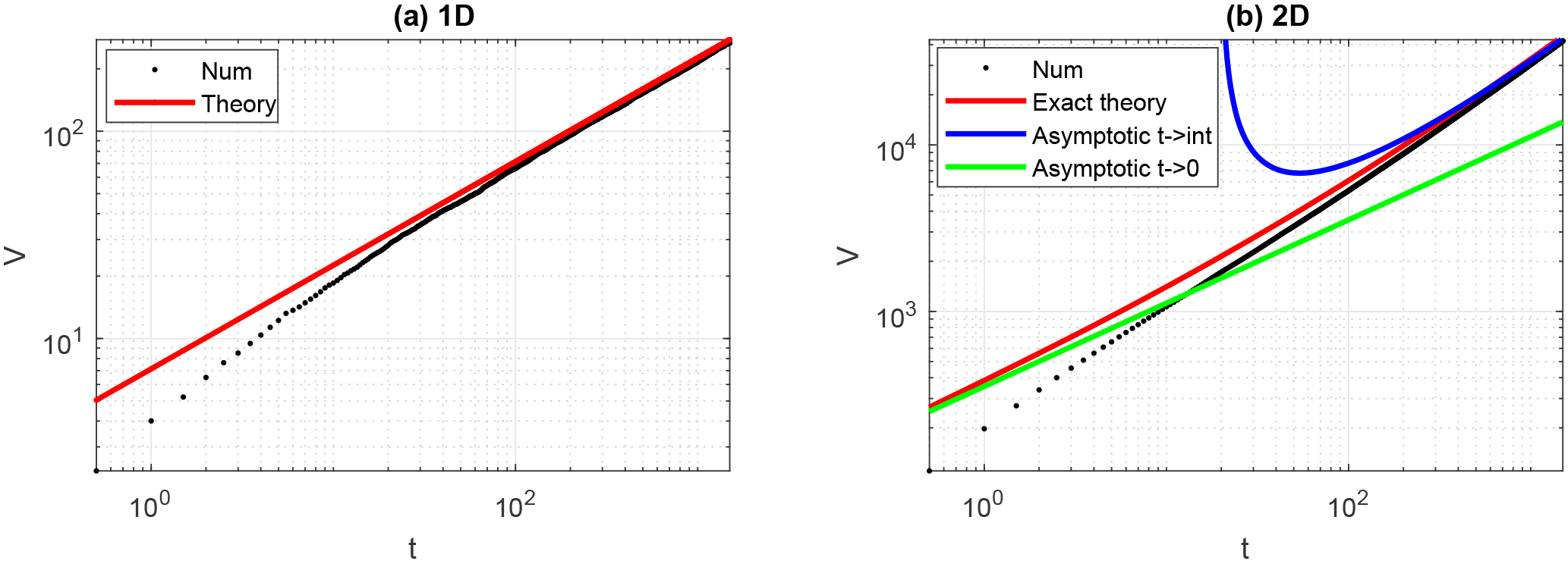
Figure 3 Comparison between theoretical expression (red, green, blue) and numerical estimates (black) of the encounter volume for a random walk in 1-D (a) and 2-D (b). In both, κ=5 and Δt=05. In 2-D, τ≅20.

The comparison between numerical simulations and theory is shown in Fig. 3. Because the numerically simulated random walk deviates significantly from the diffusive regime over short (< O(100Δt)) timescales, the agreement between numerical simulation and theory is poor at those times in both 1-D and 2-D. Once the random walkers have executed > 100 time steps, however, the dispersion reaches the diffusive regime, and the agreement between the theory (red) and numerical simulation (black) rapidly improves for both the 1-D and 2-D cases, with the two curves approaching each other at long times. In 2-D, the long-time asymptotic formula (38) works well at long times, t≫τ, as expected. The 2-D short-time asymptotic formula (green) agrees well with the exact formula (red) at short times but not with the numerical simulations (black) for the same reason as discussed above, i.e., because the numerically simulated random walk has not yet reached the diffusive regime at those times.

3 Application to the altimetric velocities in the Gulf Stream region

Sea surface height measurements made from altimetric satellites provide nearly global estimates of geostrophic currents throughout the World Oceans. These velocity fields, previously distributed by AVISO, are now available from the Copernicus Marine and Environment Monitoring Service (CMEMS) website (http://marine.copernicus.eu/), both along satellite tracks and as a gridded mapped product in both near-real and delayed time. Here we use the delayed-time gridded maps of absolute geostrophic velocities with 1∕4 deg spatial resolution and a temporal step of 1 day, and focus our attention on the Gulf Stream extension region of the North Atlantic Ocean. There, the Gulf Stream separates from the coast and starts to meander, shedding cold- and warm-core Gulf Stream rings from its southern and northern flanks. These rings are among the strongest mesoscale eddies in the ocean. However, their coherence, interaction with each other and with other flow features, and their contribution to transport, stirring and mixing are still not completely understood (Bower et al., 1985; Cherian and Brink, 2016).

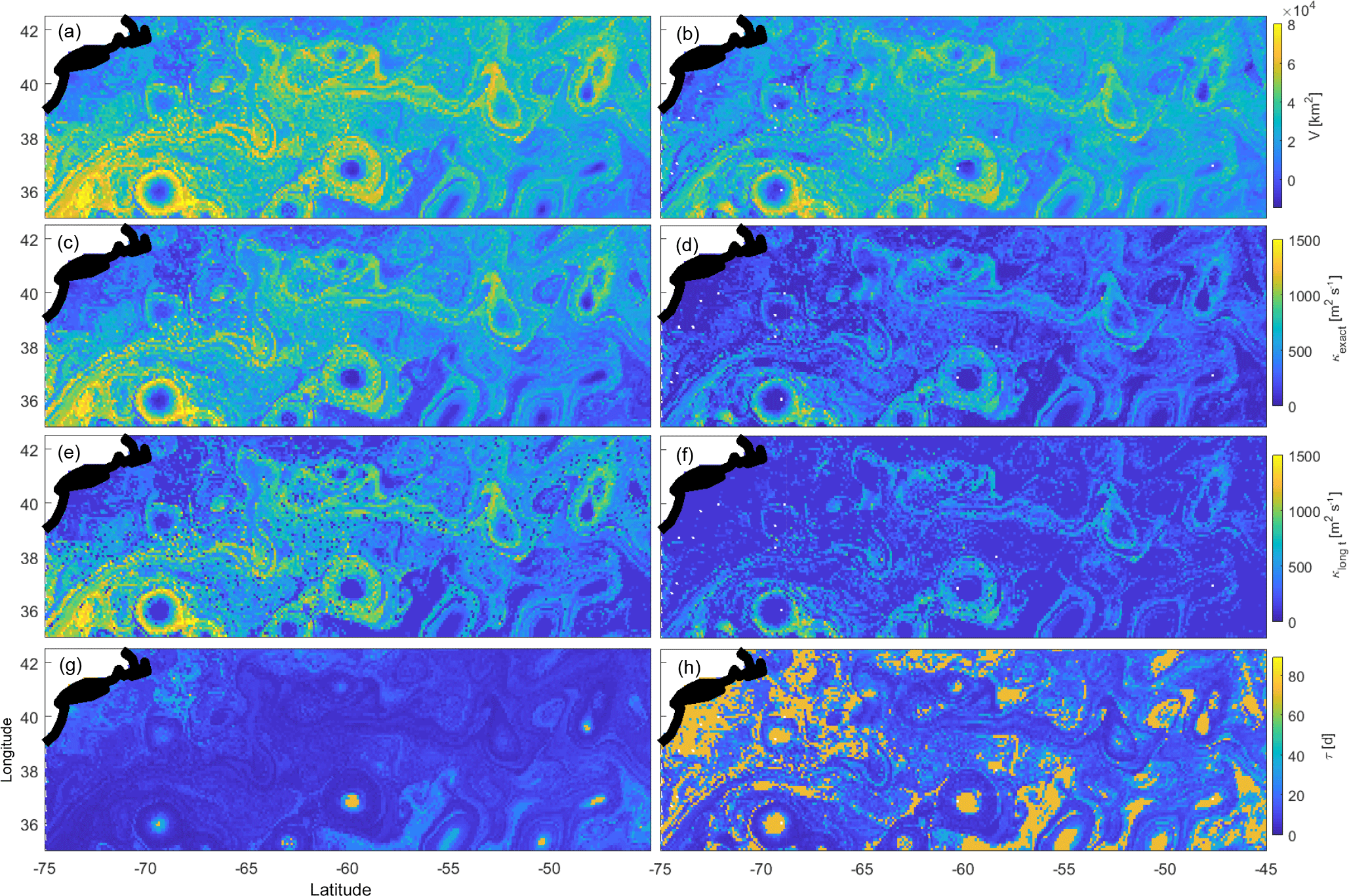
Figure 4 Encounter volume (a, b), exact diffusivity (c, d), long-time diffusivity (e, f) and diffusive timescale (g, h) for the full flow (a, c, e, g) and for the eddy component of the flow (b, d, f, h). White shows land and the thick black curve shows the coastline. The encounter volume was computed on 11 January 2015 over 90 days with an encounter radius of 30 km.

Maps showing the encounter volume for fluid parcel trajectories in the region, and the corresponding diffusivity estimates (Fig. 4), could be useful both for understanding and interpreting the transport properties of the flow, as well as for benchmarking and parameterization of eddy effects in numerical models. In our numerical simulations, trajectories were released on a regular grid with $\mathrm{d}x=\mathrm{d}y\cong \mathrm{10}$ km on 11 January 2015 and were integrated forward in time for 90 days using a fifth-order variable-step Runge–Kutta integration scheme with bi-linear interpolation between grid points in space and time. The encounter radius was chosen to be R=30 km in both the zonal and meridional directions, i.e., about a third of a radius of a typical Gulf Stream ring. Similar parameter values were used in Rypina and Pratt (2017), although our new simulation was carried out using more recent 2015 velocities instead of 1997 as in that paper.

The encounter volume field, shown in the top left panel of Fig. 4, highlights the overall complexity of the flow and identifies a variety of features with different mixing potential, most notably several Gulf Stream rings with spatially small low-V (blue) cores and larger high-V (yellow) peripheries. Although the azimuthal velocities and vorticity-to-strain ratio are large within the rings, the coherent core regions with inhibited mixing potential are small, suggesting that the coherent transport by these rings might be smaller than anticipated from the Eulerian diagnostics such as the Okubo–Weiss or closed-streamline criteria (Chelton et al., 2011; Abernathey and Haller, 2018). On the other hand, the rings' peripheries, where the mixing potential is elevated compared to the surrounding fluid, cover a larger geographical area than the cores. Thus, while rings inhibit mixing within their small cores, the enhanced mixing on the periphery might be their dominant effect. This is consistent with the results from Rypina and Pratt (2017), but a more thorough analysis is needed to test this hypothesis. Notably, the encounter volume is also large along the northern and southern flanks of the Gulf Stream jet, with two separate yellow curves running parallel to each other and a valley in between (although the curves could not be traced continuously throughout the entire region). This enhanced mixing on both flanks of the Gulf Stream extension current is reminiscent of chaotic advection driven by the tangled stable and unstable manifolds at the sides of the jet (del-Castillo-Negrete and Morrison, 1993; Rogerson et al., 1999; Rypina et al., 2007; Rypina and Pratt, 2017), and is also consistent with the existence of critical layers (Kuo, 1949; Ngan and Sheppard, 1997).

We now apply the asymptotic formula (38) to convert the encounter volume to diffusivity. Because Eq. (38) is not invertible analytically, we converted V to κ numerically using a look-up table approach. More specifically, we used Eq. (38) to compute theoretically predicted V values at time T= 90 days for a wide range of κs spanning all possible oceanographic values from 0 up to 10⁹ cm² s⁻¹, and we used the resulting look-up table to assign the corresponding κ values to V values in the third row of Fig. 4. Note that, instead of the long-time asymptotic formula (38) (as in the third row of Fig. 4), it is also possible to use the exact formulas (28)–(29) to convert V to κ via a look-up table approach. The resulting exact diffusivities, shown in the second row of Fig. 4, are similar to the long-time asymptotic values (third row). Because both exact and asymptotic formulas were derived under the assumption of a diffusive random walk, neither should work well in regions with a non-diffusive behavior. The asymptotic formula has the advantage of being simpler and it also provides for a numerical estimate of the “long-time-limit” timescale, τ, shown in the bottom row of Fig. 4.

As expected, the diffusivity maps in the second and third rows of Fig. 4, which resulted from converting V to κ using (28)–(29) or (38), respectively, have the same spatial variability as the V-map, with large κ at the peripheries of the Gulf Stream rings and at the flanks of the Gulf Stream and small κ at the cores of the rings, near the Gulf Stream centerline and far away from the Gulf Stream current, where the flow is generally slower. The diffusivity values range from O(10⁵) to O(10⁷) cm² s⁻¹. Using the 1971 Okubo's diffusivity diagram and scaling law, κ_Okubo[cm² s⁻¹]= 0.0103 L[cm]^1.15, our diffusivity values correspond to spatial scales from 10 to 650 km, thus spanning the entire mesoscale range. This is not surprising considering the Lagrangian nature of our analysis, where trajectories inside the small (<50 km) low-diffusion eddy cores stay within the cores for the entire integration duration (90 days), whereas trajectories in the high-diffusivity regions near the ring peripheries and at the flanks of the Gulf Stream jet cover large distances, sometimes >650 km, over 90 days.

The performances of the exact and asymptotic diffusive formulas vary greatly throughout the domain, with better/poorer performances in high-/low-V areas. This is because in the low-V areas, the behavior of fluid parcels is non-diffusive, so the diffusive theoretical formulas work poorly. The breakdown of the long-time asymptotic formula is evident in the fourth row of Fig. 4, which shows the corresponding long-time scales, τ (from Eq. 35), throughout the domain. As suggested by our 2-D random walk simulations, the long-time asymptotic diffusive formula only works well when t≫τ, but in reality τ values are < 9 days (1∕10 of our integration time) only in the highest-V regions, and are much larger everywhere else, reaching values of ≅90 days within the cores of the Gulf Stream rings. More detailed comparison between theory, both exact and asymptotic, and numerical V(t) is shown in Fig. 5 for three reference trajectories that are initially located inside the core, on the periphery, and outside of a Gulf Stream ring (black, red, and blue, respectively) centered at approximately 36.8^∘ N and 60^∘ W. Clearly, the diffusive theory works poorly for the trajectory inside the eddy core (black curve). The agreement is better for the blue curves and even better for the red curves, corresponding to trajectories outside and on the periphery of the eddy, although deviations between the theory and numerics are still visible, raising questions about the general validity of the diffusive approximation in ocean flows on timescales of a few months.

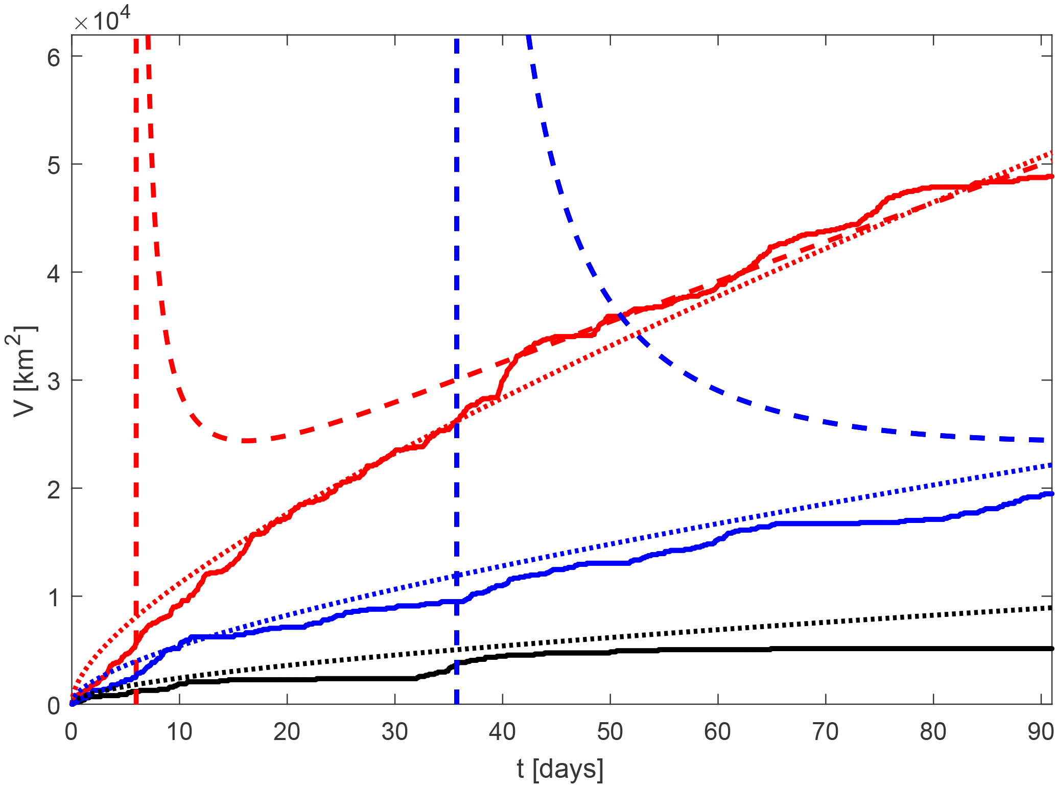
Figure 5 Comparison between numerically computed V (solid) and the exact (dotted) and long-time diffusive formulas (dashed) with the corresponding κ for the three reference trajectories located in the core, periphery and outside (black, red, blue) of a Gulf Stream ring.

The non-diffusive nature of the parcel motion over 90 days is because ocean eddies have finite lengthscales and timescales, so a variety of different transport regimes generally occur before separating parcels become uncorrelated and transport becomes diffusive, as in a random walk. At very short times the motion of fluid parcels is largely governed by the local velocity shear, so the resulting transport regime is ballistic, i.e., D∝T² and V∝T (Rypina and Pratt, 2017). At longer times, when velocity shear can no longer be assumed constant in space and time, the regime may transition to a local Richardson regime (i.e., D∝t³), where separation at a given scale is governed by the local features of a comparable scale (Richardson, 1926; Bennett, 1984; Beron-Vera and LaCasce, 2016), or to a non-local chaotic-advection spreading regime (i.e., D∝exp(λt)), where separation is governed by the large-scale flow features (Bennett, 1984; Rypina et al., 2010; Beron-Vera and LaCasce, 2016). The kinetic energy spectrum of a flow indicates whether a local or non-local regime will be relevant. The chaotic transport regime is generally expected to occur in mesoscale-dominated eddying flows, such as, for example, AVISO velocity fields, over timescales of a few eddy winding times. At times long enough for particles to sample many different flow features, such as Gulf Stream meanders or mesoscale eddies in the AVISO fields, the velocities of the neighboring particles become completely uncorrelated, and transport finally approaches the diffusive regime. With the mesoscale eddy turnover time being on the order of several weeks, it often takes longer than 90 days to reach the diffusive regime.

A number of diffusivity estimates other than Okubo's have been made for the Gulf Stream extension region (e.g., Zhurbas and Oh, 2004; LaCasce, 2008; Rypina et al., 2012; Abernathey and Marshall, 2013; Klocker and Abernathey, 2014; or Cole et al., 2015). These estimates are based on surface drifters (Zhurbas and Oh, 2004; LaCasce, 2008; Rypina et al., 2012), satellite-observed velocity fields (Abernathey and Marshall, 2013; Klocker and Abernathey, 2014; Rypina et al., 2012), and Argo float observations (Cole et al., 2015), and they use either the spread of drifters or the evolution of simulated or observed tracer fields to deduce diffusivity. The resulting diffusivities are spatially varying and span 2 orders of magnitude, from 2×10⁴ m² s⁻¹ in the most energetic regions in the immediate vicinity of the Gulf Stream and its extension, to 10³ m² s⁻¹ in less energetic areas, to 200 m² s⁻¹ in the coastal areas of the Slope Sea. Diffusivity estimates vary significantly depending on the initial tracer distribution used (Abernathey and Marshall, 2013) and depend on whether the suppression by the mean current has been taken into account (Klocker and Abernathey, 2014). The diffusivity tensor has also been shown to be anisotropic, with a large anisotropy ratio near the Gulf Stream (Rypina et al., 2012). Data resolution and coverage, as well as the choice of timescales and lengthscales also play a role in defining κ value (Cole at al., 2015). All of these issues complicate the reconciliation of different diffusivity estimates. Nevertheless, ignoring these complications for a moment, and avoiding the smallest diffusivities in those geographical areas of Fig. 4 where the diffusive approximation is invalid, our O(10³ m² s⁻¹) encounter-volume-based diffusivity estimates tend to be in the middle of the range of available estimates for the western North Atlantic. Although not inconsistent with other estimates, the encounter volume method did not predict diffusivities to reach values of 10⁴ m² s⁻¹ anywhere within the considered geographical domain.

Because the action of the real ocean velocity field on drifters or tracers is generally not exactly diffusive, all methods simply fit the diffusive approximation to the corresponding variable of interest, such as particle dispersion, tracer variance, or, in our case, encounter volume. The analytic form of the diffusive approximation is, however, different for different variables and different flow regimes. For example, for a diffusive random walk regime, dispersion grows linearly with time, whereas the growth of the encounter volume is nonlinear, as defined by Eq. (38). This generally leads to different diffusivity estimates resulting from different methods. In other words, the diffusivity value that fits best to the observed particle dispersion at 90 days does not necessarily provide the best fit to the observed encounter volume at 90 days, and vice versa.

To illustrate this more rigorously, we consider a linear strain flow,

$$\begin{array}{ll}{\displaystyle }& {\displaystyle }u=\mathit{\alpha }x,\\ {\displaystyle }& {\displaystyle }v=-\mathit{\alpha }y,\end{array}$$

with a constant strain coefficient α. The particle trajectories are given by $x=x_{\mathrm{0}}{e}^{\mathit{\alpha }\mathrm{t}},y=y_{\mathrm{0}}{e}^{-\mathit{\alpha }\mathrm{t}}$ where x₀, y₀ are particles' initial positions. The dispersion of a small cluster of particles that are initially uniformly distributed within a small square of side length 2dx is

$${\displaystyle }D=\langle {\left(X-\stackrel{\mathrm{‾}}{X}\right)}^{\mathrm{2}}+{\left(Y-\stackrel{\mathrm{‾}}{Y}\right)}^{\mathrm{2}}\rangle ,$$

where $X=x-x_{\mathrm{0}}$ and $Y=y-y_{\mathrm{0}}$ are displacements of particles from their initial positions and the overbar denotes the ensemble mean. Since the linear strain velocity remains unchanged in a reference frame moving with a particle, without loss of generality we can restrict our attention to a cluster that is initially centered at the origin, so $\stackrel{\mathrm{‾}}{X}=\stackrel{\mathrm{‾}}{Y}=\mathrm{0}$. In the long-time limit, when $e^{\mathit{\alpha }\mathrm{t}}\gg \mathrm{1}\gg e^{-\mathit{\alpha }\mathrm{t}}$, the dispersion becomes

$${\displaystyle }D=\mathrm{1}/\mathrm{3}\mathrm{d}{x}^{\mathrm{2}}{e}^{\mathrm{2}\mathit{\alpha }t}.$$

If one is using a diffusive fit,

$${\displaystyle }D=\mathrm{4}{\mathit{\kappa }}_{\mathrm{D}}t,$$

to approximate diffusivity, then the resulting diffusivity is

$${\displaystyle }{\mathit{\kappa }}_{\mathrm{D}}={\displaystyle \frac{\mathrm{d}{x}^{\mathrm{2}}{e}^{\mathrm{2}\mathit{\alpha }t}}{\mathrm{12}t}}.$$

On the other hand, the encounter volume for the linear strain flow is

$${\displaystyle }V=\mathrm{2}\mathit{\alpha }{R}^{\mathrm{2}}t,$$

whereas the long-time diffusive fit is

$${\displaystyle }V={\displaystyle \frac{\mathrm{4}\mathit{\pi }{\mathit{\kappa }}_{\mathrm{V}}t}{\ln t/\mathit{\tau }}},$$

yielding

$${\displaystyle }{\mathit{\kappa }}_{\mathrm{V}}=-{\displaystyle \frac{\mathit{\alpha }{R}^{\mathrm{2}}\mathrm{ProductLog}\left(-\frac{\mathit{\pi }{e}^{\mathrm{2}\mathit{\gamma }}}{\mathrm{2}\mathit{\alpha }t}\right)}{\mathrm{2}\mathit{\pi }}}$$

where the function ProductLog(z), also known as the Lambert function, is a solution to z=we^w. Because κ_D is exponential in time, while κ_V is not, κ_D always becomes larger than κ_V at large t.

Of course, real oceanic flows are more complex than the simple linear strain example. However, for flows that are in a state of chaotic advection, exponential separation between neighboring particles will occur and the dispersion will grow exponentially in time, as in the linear strain example. Although we do not have a formula for the encounter volume for a chaotic advection regime, the linear strain example suggests that the encounter volume growth will likely be slower than exponential. Thus, for a chaotic advection regime, the dispersion-based diffusivity could be expected to be larger than the encounter-volume-based diffusivity. This can potentially explain the smaller encounter-volume-based diffusivity values in Fig. 4 compared to other available estimates from the literature. Numerical simulations (not shown) using an analytic Duffing oscillator flow, which features chaotic advection, indeed produced smaller encounter-volume-based diffusivity than dispersion-based diffusivity, in agreement with our arguments above. The AVISO velocities are dominated by the mesoscales rather than submesoscales, and the 90-day time interval is about a few mesoscale eddy winding times; thus, this flow satisfies all the pre-requisites for the chaotic advection to occur. Finally, the particle trajectories that we used to produce Fig. 4 can be grouped into small clusters (we are using the encounter radius R= 30 km as a cluster radius for consistency) to estimate their dispersion and infer diffusivity from its slope. Consistent with our arguments above, the resulting dispersion-based diffusivities in Fig. 6 are larger than the encounter-volume-based diffusivities in Fig. 4 and reach values of O(10⁴ m² s⁻¹) in the energetic regions of the Gulf Stream and its extension, in agreement with the previous diffusivity estimates from the literature. In applications where the number of encounters is a more important quantity than the spread of particles, the encounter-volume-based diffusivity might be a more appropriate estimate to use.

Figure 6 Dispersion-based diffusivity, κ_D.

In the left panels of Fig. 4 we used the full velocity field to advect trajectories, so both the mean and the eddies contributed to the resulting encounter volumes and the corresponding diffusivities. But what is the contribution of the eddy field alone to this process? To answer this question, we have performed an additional simulation in the spirit of Rypina et al. (2012), where we advected trajectories using the altimetric time-mean velocity field, and then subtracted the resulting encounter volume, V_mean, from the full encounter volume, V. The result characterizes the contribution of eddies, although strictly speaking $V_{\mathrm{eddy}}\ne V-V_{\mathrm{mean}}$ because of nonlinearity. Note also that because we are interested in the Lagrangian-averaged effects of eddies following fluid parcels, V_eddy cannot be estimated by simply advecting particles by the local eddy field alone (see an extended discussion of this effect in Rypina et al., 2012). Not surprisingly, the eddy-induced encounter volumes (upper right panel of Fig. 4) are smaller than the full encounter numbers, with the largest decrease near the Gulf Stream current, where both the mean velocity and the mean shear are large. In other geographical areas, specifically at the peripheries of the Gulf Stream rings, the decrease in V is less significant, so the resulting map retains its overall qualitative spatial structure. The same is true for the diffusivities in the second and third rows of Fig. 4. The overall spatial structure of the eddy diffusivity is preserved and matches that in the left panels, but the values decrease, with the largest differences near the Gulf Stream, where some diffusivity values are now O(10⁶) instead of O(10⁷) cm² s⁻¹. In contrast, κ only decreases, on average, by a factor of 2 (instead of an order of magnitude) near the peripheries of the Gulf Stream rings. The long-time diffusive timescale τ generally increases, and the ratio t∕τ generally decreases throughout the domain, but the long-time asymptotic formula (38) still works well in high-V regions, specifically on the peripheries of the Gulf Stream rings where τ is still significantly less than t.

4 Discussion and summary

With many new diagnostics being developed for characterizing mixing in fluid flows, it is important to connect them to the well-established conventional techniques. This paper is concerned with understanding the connection between the encounter volume, which quantifies the mixing potential of the flow, and diffusivity, which quantifies the intensity of the down-gradient transfer of properties. Intuitively, both quantities characterize mixing, and it is natural to expect a relationship between them, at least in some limiting sense. Here, we derived this anticipated connection for a diffusive process, and we showed how this connection can be used to produce maps of spatially varying diffusivity and to gain new insights into the mixing properties of eddies and the particle spreading regime in realistic oceanic flows.

When applied to the altimetry-based velocities in the Gulf Stream region, the encounter volume and diffusivity maps show a number of interesting physical phenomena related to transport and mixing. Of particular interest are the transport properties of the Gulf Stream rings. The materially coherent Lagrangian cores of these rings, characterized by very small diffusivity, are smaller than expected from earlier Eulerian diagnostics (Chelton et al., 2011). The periphery regions with enhanced diffusivity are, on the other hand, large, raising a question about whether the rings, on average, act to preserve coherent blobs of water properties or to speed up the mixing. The encounter volume, through the derived connection to diffusivity, might provide a way to address this question and to quantify the two effects, clarifying the role of eddies in transport and mixing.

Our encounter-volume-based diffusivity estimates are within the range of other available estimates from the literature, but are not among the highest. We provided an intuitive explanation for why the encounter-volume-based diffusivities might be smaller than the dispersion-based diffusivities, and we supported our explanation with theoretical developments based on a linear strain flow, and with numerical simulations. We note that in problems where the encounters between particles are of interest, rather than the particle spreading, the encounter-volume-based diffusivities would be more appropriate to use than the conventional dispersion-based estimates.

Reliable data-based estimates of eddy diffusivity are needed for parameterizations in numerical models. The conventional estimation of diffusivity from Lagrangian trajectories by calculating particle dispersion requires large numbers of drifters or floats (LaCasce, 2008). It would be useful to have a technique that would work with fewer instruments. The derived connection between encounter volume and diffusivity might help in achieving this goal. Specifically, one could imagine that if an individual drifting buoy were equipped with an instrument that would measure its encounter volume – the volume of fluid that came in contact with the buoy over time t – then the resulting encounter volume could be converted to diffusivity using the derived connection. This would allow estimation of diffusivity using a single instrument.

In the field of social encounters, it is becoming possible to construct large data sets by tracking cell phones, smart transit cards (Sun et al., 2013), and bank notes (Brockmann et al., 2006). As was the case for the Gulf Stream trajectories, some of the behavior appears to be diffusive and some not so. Where diffusive/random walk behavior is relevant, it may be easier to accumulate data on close encounters rather than on other metrics using, for example, autonomous vehicles and instruments that are able, through local detection capability, to count foreign objects that come within a certain range.