the Creative Commons Attribution 4.0 License.
the Creative Commons Attribution 4.0 License.
 | 29 Mar 2018
Complex interplay between stress perturbations and viscoelastic relaxation in a two-asperity fault model
Emanuele Lorenzano
Michele Dragoni
We consider a plane fault with two asperities embedded in a shear zone, subject to a uniform strain rate owing to tectonic loading. After an earthquake, the static stress field is relaxed by viscoelastic deformation in the asthenosphere. We treat the fault as a discrete dynamical system with 3 degrees of freedom: the slip deficits of the asperities and the variation of their difference due to viscoelastic deformation. The evolution of the fault is described in terms of inter-seismic intervals and slip episodes, which may involve the slip of a single asperity or both. We consider the effect of stress transfers connected to earthquakes produced by neighbouring faults. The perturbation alters the slip deficits of both asperities and the stress redistribution on the fault associated with viscoelastic relaxation. The interplay between the stress perturbation and the viscoelastic relaxation significantly complicates the evolution of the fault and its seismic activity. We show that the presence of viscoelastic relaxation prevents any simple correlation between the change of Coulomb stresses on the asperities and the anticipation or delay of their failures. As an application, we study the effects of the 1999 Hector Mine, California, earthquake on the post-seismic evolution of the fault that generated the 1992 Landers, California, earthquake, which we model as a two-mode event associated with the consecutive failure of two asperities.
- Article
(1695 KB) - Full-text XML
- BibTeX
- EndNote


Asperity models have long been acknowledged as an effective means to describe many aspects of fault dynamics (Lay et al., 1982; Scholz, 2002). In such models, it is assumed that the bulk of energy release during an earthquake is due to the failure of one or more regions on the fault characterized by a high static friction and a velocity-weakening dynamic friction. The stress build-up on the asperities is governed by the relative motion of tectonic plates. Earthquakes that have been ascribed to the slip of two asperities are the 1964 Alaska earthquake (Christensen and Beck, 1994); the 1992 Landers, California, earthquake (Kanamori et al., 1992); the 2004 Parkfield, California, earthquake (Twardzik et al., 2012); and the 2010 Maule, Chile, earthquake (Delouis et al., 2010).
In the framework of asperity models, a critical role is played by stress accumulation on the asperities, fault slip at the asperities and stress transfer between the asperities. Accordingly, fault dynamics can be fruitfully investigated via discrete dynamical systems whose essential components are the asperities (Ruff, 1992; Turcotte, 1997). Such an approach reduces the number of degrees of freedom required to describe the dynamics of the system, that is, the evolution of the fault (in terms of slip and stress distribution) during the seismic cycle; also, it allows the visualization of the state of the fault and to follow its evolution via a geometrical approach, by means of orbits in the phase space. Finally, a finite number of dynamic modes can be defined, each one describing a particular phase of the evolution of the fault (e.g. tectonic loading, seismic slip, after-slip). Asperity models are capable of reproducing the essential features of the seismic source, while sparing the more complicated characterization based on continuum mechanics.
In a number of recent works, modelling of different mechanical phenomena in a two-asperity fault system has been addressed, such as stress perturbations due to surrounding faults (Dragoni and Piombo, 2015) and the radiation of seismic waves (Dragoni and Santini, 2015). In these models, the fault is treated as a discrete dynamical system with four dynamic modes: a sticking mode, corresponding to stationary asperities, and three slipping modes, associated with the separate or simultaneous failure of the asperities.
In the framework of a discrete fault model, the impact of viscoelastic relaxation was first studied by Amendola and Dragoni (2013) and then further investigated by Dragoni and Lorenzano (2015), who considered a fault with two asperities of different strengths. The authors discussed the features of the seismic events predicted by the model and showed how the shape of the associated source functions is related to the sequence of dynamic modes involved. In turn, the observation of the moment rate provides an insight into the state of the system at the beginning of the event, that is, the particular stress distribution on the fault from which the earthquake takes place.
However, no fault can be considered isolated; in fact, any fault is subject to stress perturbations associated with earthquakes on neighbouring faults (Harris, 1998; Stein, 1999; Steacy et al., 2005). Whenever a fault slips, the stress field in the surrounding medium is altered. As a result, the occurrence time and the magnitude of next earthquakes may change with respect to the unperturbed condition, which is governed by tectonic loading.
The aim of the present paper is to discuss the combined effects of viscoelastic relaxation and stress perturbations on a two-asperity fault in the framework of a discrete fault model. In order to deal with such a problem, we base our work on the results achieved by Dragoni and Piombo (2015) and Dragoni and Lorenzano (2015). In the former work, the authors considered a two-asperity fault with purely elastic rheology and discussed the effect of stress perturbations due to earthquakes on neighbouring faults. The fault was treated as a discrete dynamical system whose state is described by two variables, the slip deficits of the asperities. In the latter work, viscoelastic relaxation on the fault was dealt with by adding a third state variable, the variation in the difference between the slip deficits of the asperities during inter-seismic intervals. In the present paper, we introduce stress perturbations as modelled by Dragoni and Piombo (2015) in the framework of the two-asperity fault considered by Dragoni and Lorenzano (2015). Accordingly, the present work represents a three-dimensional generalization of the model devised by Dragoni and Piombo (2015). Elastic wave radiation and additional constraints on the state of the fault are taken into account, as further developments with respect to previous works.
In the framework of the present model, seismic events generated by the fault are discriminated according to the number and sequence of slipping modes involved and the seismic moment released; these features are related to the particular state of the system at the beginning of the inter-seismic interval preceding the event. We discuss how stress perturbations affect the evolution of the fault in terms of changes in the state of the system and in the duration of the inter-seismic time, highlighting the complications arising from the ongoing post-seismic deformation process with respect to the purely elastic case considered by Dragoni and Piombo (2015). As an application, we consider the stress perturbation imposed by the 1999 Hector Mine, California, earthquake (Jónsson et al., 2002; Salichon et al., 2004) to the fault that caused the 1992 Landers, California, earthquake, which we model as a two-mode event due to the consecutive failure of two asperities and that was followed by remarkable viscoelastic relaxation (Kanamori et al., 1992; Freed and Lin, 2001). We propose a means to estimate the stress transfer from the knowledge of the relative positions and faulting styles of the two faults. As a further novelty with respect to the work presented by Dragoni and Lorenzano (2015), we show how the knowledge of the time interval elapsed after the 1999 earthquake can be used to constrain the admissible set of states that may have given rise to the 1992 event. We discuss the possible subsequent evolution of the Landers fault after the stress transfer from the Hector Mine earthquake, pointing out the main differences with respect to an unperturbed scenario.
We consider a plane fault containing two asperities of equal areas A and different strengths that we name asperity 1 and asperity 2 (Fig. 1). The fault is enclosed in a homogeneous and isotropic shear zone behaving as a Poisson solid and is subject to a uniform strain rate owing to the relative motion of two tectonic plates, taking place at a constant rate V. In order to describe the viscoelastic relaxation in the asthenosphere, we assume a Maxwell viscoelastic behaviour with a characteristic relaxation time Θ. Finally, we characterize the seismic efficiency of the fault by means of an impedance γ. All quantities are expressed in non-dimensional form.
In the present model we do not consider aseismic slip on the fault. It has been treated in the framework of a discrete fault model by Dragoni and Lorenzano (2017), who considered a region slipping aseismically for a finite time interval and calculated the effect on the stress distribution and the subsequent evolution of the fault. Of course, if the amplitude of aseismic slip has the same order of magnitude as that of seismic slip, the fault evolution may be affected.
In accordance with the assumptions of asperity models, we ascribe the generation of earthquakes on the fault to the failure of the sole asperities, neglecting any contribution of the surrounding weaker region to the seismic moment. Also, we do not describe friction, slip and stress at every point of the fault, but only consider their average values on each asperity.
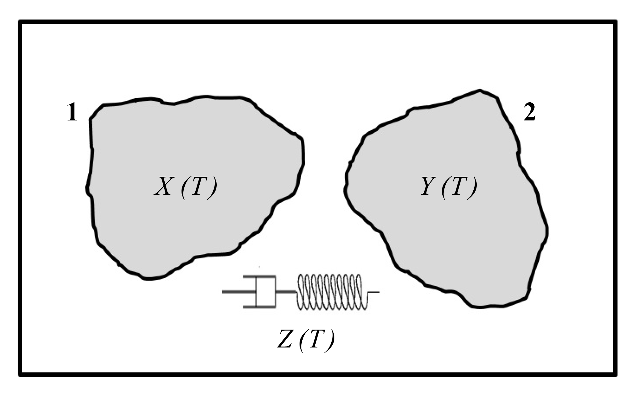
Figure 1Sketch of the model of a plane fault with two asperities. The rectangular frame is the fault border. The state of the asperities is described by their slip deficits X(T) and Y(T), while the variable Z(T) represents the temporal variation of the difference between the slip deficits of the asperities due to viscoelastic deformation in the inter-seismic interval following an earthquake on the fault.
The fault is treated as a dynamical system with three state variables, functions of time T: the slip deficits X(T) and Y(T) of asperity 1 and 2, respectively, and the variable Z(T) representing the temporal variation of the difference Y−X between the slip deficits of the asperities during inter-seismic intervals of the fault, due to the stress redistribution associated with viscoelastic relaxation in the asthenosphere. The slip deficit of an asperity is defined as the slip that an asperity should undergo at a given instant in time in order to recover the relative displacement of tectonic plates that occurred up to that moment.
We assume the simplest form of rate-dependent friction and associate the asperities with constant static and dynamic frictions, the latter considered as the average value during slip. The static friction on asperity 2 is a fraction β of that on asperity 1 and dynamic frictions are a fraction ϵ of static frictions for both asperities. Letting fs1 and fd1 be the static and dynamic frictions on asperity 1, respectively, and fs2 and fd2 be the static and dynamic frictions on asperity 2, respectively, we have
We acknowledge that the values of friction after a seismic event might be different from the initial ones, even though it is probable that the change is remarkable only after several seismic cycles. We neglect this possible change, because we focus on other sources of irregularity in the seismic cycles. However, the model could easily incorporate a change in friction after each event: new values could be given to static and dynamic frictions after the event and the subsequent evolution could be calculated accordingly.
During a global stick mode, the tangential forces acting on the asperities in the slip direction are (in units of static friction on asperity 1)
In these expressions, the terms −X and −Y represent the effect of tectonic loading and have the same sign for both asperities, whereas the terms ±αZ are the contributions of stress transfer between the asperities. In the framework of the present model, stress is transferred by one asperity to the other as a result of co-seismic slip; in the subsequent inter-seismic interval, the static stress field generated by asperity slip undergoes a certain amount of relaxation owing to viscoelasticity. The parameter α is a measure of the degree of coupling between the asperities: for smaller values of α, the stress transfer from one asperity to the other is less efficient. In the limit case α=0, the asperities are completely independent from one another and the slip of one of them does not affect the state of the other: the evolution of the asperities is thus governed by tectonic loading only. By comparison with a model based on continuum mechanics, the specific value of α can be estimated as (Dragoni and Tallarico, 2016)
where A is the area of the asperities, v is the velocity of the tectonic plates, s is the tangential traction (per unit moment) imposed on one asperity by the slip of the other and is the tangential strain rate on the fault due to tectonic loading.
An effective way to characterize fault mechanics is provided by the concept of Coulomb stress (Stein, 1999). It is defined as the difference between the shear stress σt in the direction of fault slip and the static friction τs on the fault surface:
Accordingly, σC is negative during an inter-seismic interval and a seismic event occurs when σC vanishes. In our model, the presence of two asperities makes it necessary to assign a value of Coulomb stress to each of them. By definition, the Coulomb forces on asperity 1 and 2 are, respectively,
Using Eq. (2), they can be rewritten as
To sum up, the system is described by the set of six parameters α, β, γ, ϵ, Θ and V, with α≥0, , γ≥0, , Θ>0 and V>0. At any instant T in time, the state of the system may be univocally expressed by the tern or by one of the couples .
When considering the fault dynamics during the seismic cycle, it is possible to identify four dynamic modes, each one described by a different system of autonomous ODEs (ordinary differential equations): a sticking mode (00), corresponding to stationary asperities, and three slipping modes, associated with the slip of asperity 1 alone (mode 10), the slip of asperity 2 alone (mode 01) and the simultaneous slip of the asperities (mode 11). A seismic event generally consists of n slipping modes and involves one or both the asperities.
The sticking region
The sticking region of the system is defined as the set of states in which both asperities are stationary. During a global stick phase (mode 00), the rates , and are negligible with respect to their values when the asperities are slipping; thus, the sticking region is a subset of the space XYZ.
The slip of asperity 1 occurs when
while the slip of asperity 2 takes place when
Combining these conditions with the expressions (2) of the forces, we obtain two planes in the XYZ space,
which we name Π1 and Π2, respectively. Of course, the Coulomb forces and vanish on Π1 and Π2, respectively; furthermore, their gradients
are orthogonal to Π1 and Π2, respectively.
We exclude overshooting during the slipping modes: accordingly, we assume X≥0 and Y≥0. As a consequence, the tangential forces on the asperities must always be in the same direction as the velocity of tectonic plates, i.e. F1≤0 and F2≤0. From Eq. (2), the limit cases F1=0 and F2=0 correspond to two planes in the XYZ space,
which we name Γ1 and Γ2, respectively.
To sum up, the sticking region of the system is the subset of the XYZ space enclosed by the planes , Γ1, Γ2, Π1 and Π2: a convex hexahedron H. Its vertices are the origin and the points
The sticking region is shown in Fig. 2 for a particular choice of the parameters α and β. Its volume can be expressed as a function of the parameters of the system as . Accordingly, the subset of the state space corresponding to stationary asperities decreases with the degree of coupling between the asperities and with the asymmetry of the system (β→0). By definition, every orbit of mode 00 is enclosed within H and eventually reaches one of its faces AECD or BCDF, belonging to the planes Π1 and Π2, respectively, where an earthquake starts. In these cases, the system switches from mode 00 to mode 10 or mode 01, respectively. In the particular case in which the orbit of mode 00 reaches the edge CD, the system passes from mode 00 to mode 11.
Let P0∈H be the state of the system at the beginning of an inter-seismic interval. The specific location of P0 inside the sticking region allows the prediction of the first slipping mode involved in the next seismic event on the fault. In fact, Dragoni and Lorenzano (2015) illustrated the existence of a transcendental surface Σ within H, expressed by the equation
where W is the Lambert function with arguments
The surface Σ divides H in two subsets H1 and H2 (Fig. 3). The seismic event starts with mode 10 if P0∈H1 or with mode 01 if P0∈H2; in the particular case in which P0∈Σ, the seismic event starts with mode 11.
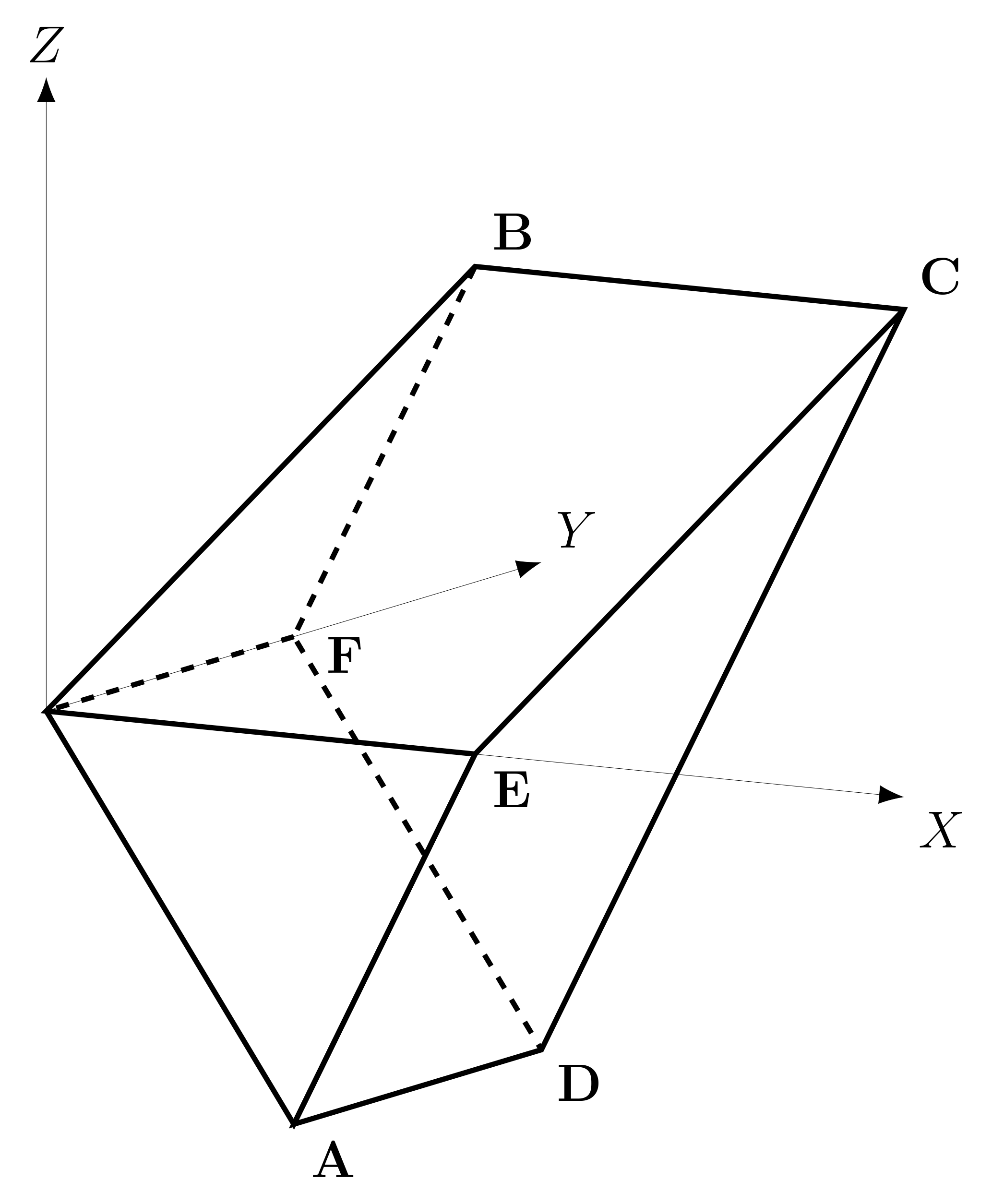
Figure 2The sticking region of the system, defined as the subset of the state space XYZ in which both asperities are at rest: a convex hexahedron H .
Mode 00 terminates at a point P1 on the face AECD or BCDF of H. The number and sequence of slipping modes involved in the subsequent seismic event can be discriminated from the specific position of P1. If we consider the face AECD (Fig. 4), the earthquake will be a one-mode event 10 if P1 belongs to the trapezoid Q1; it will be a two-mode event 10-01 if P1 belongs to the segment s1; it will be a three-mode event 10-11-01 or 10-11-10 if P1 belongs to the trapezoid R1, where the precise sequence must be evaluated numerically and depends on the particular combination of the parameters α, β, γ and ϵ. The remaining portion of the face would lead to overshooting. Analogous considerations can be made for the subsets Q2, s2 and R2 on the face BCDF. In the particular case in which P1 belongs to the edge CD, the earthquake will be a two-mode event 11-01. In fact, by definition, friction on asperity 2 is smaller than friction on asperity 1 (); if the asperities start slipping simultaneously, asperity 1 is then bound to stop the first, while asperity 2 continues to slip. As a result, mode 11 is followed by mode 01 and the slip of the weaker asperity has a longer duration. The opposite would hold if asperity 2 were stronger than asperity 1 (β>1), so that the slip event resulting from states P1∈CD would be a two-mode event 11-10.

Figure 3The surface Σ that splits the sticking region H in two subsets H1 (below) and H2 (above) (α=1, β=1, VΘ=1). It allows the first slipping mode during an earthquake to be discriminated.

Figure 4The faces AECD and BCDF of the sticking region H, where seismic events start, and their subsets (α=1, β=1, γ=1, ϵ=0.7). The events taking place on the face AECD (BCDF) start with mode 10 (01). The trapezoids Qi correspond to events involving a single asperity; the segments si correspond to events associated with the consecutive slips of the asperities; the trapezoids Ri correspond to events involving the simultaneous slips of the asperities.
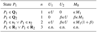
In addition, the knowledge of the position of P1 allows the total amount of slip of the asperities and the seismic moment associated with the earthquake to be established. Let us consider an event made up of n dynamic modes and let be the state of the system at time T=Ti, when the ith mode starts . The final slip amplitudes of asperity 1 and 2 are, respectively,
Accordingly, the final seismic moment can be calculated as
where M1 and U are the seismic moment and slip amplitude associated with a one-mode event 10 in the limit case γ=0, respectively, with
The possible values of U1,U2 and M0 are summarized in Table 1: the effect of wave radiation is characterized by means of the quantity
where Ts is the duration of slip in a one-mode event (Dragoni and Santini, 2015).
As for the evolution of the variable Z(T) during the earthquake, it changes according to the equation , since the relaxation process is negligible during the slip of the asperities.
We now consider the perturbations of the state of the fault caused by the coseismic slip on surrounding faults. Following Dragoni and Piombo (2015), we assume that (1) the perturbations occur during an inter-seismic interval; (2) the stress transfer takes place over a time interval negligible with respect to the duration of the inter-seismic interval; and (3) at the time of the perturbation, the state of the fault is sufficiently far from the failure conditions and the stress transfer is small enough that the onset of motion of either asperity is not achieved immediately.
Table 1Final slip amplitudes U1 and U2 of asperity 1 and 2 and seismic moment M0 during a seismic event made up of n slipping modes, as a function of the state P1 where the event started. The entry e.n. is the abbreviation for evaluated numerically.
Let be the state of the fault at the time of the perturbation. Generally speaking, the system undergoes a transition to a new state
Since the stress transfer takes place over a time interval short with respect to the inter-seismic interval (assumption 2), viscoelastic relaxation is negligible during the perturbation and the rheology can be reasonably considered as purely elastic as the perturbation takes place. Accordingly, we set
The change of state is then associated with a vector in the XYZ space:
The components of ΔR generally have different magnitudes and may have different signs, as a consequence of the inhomogeneity of the stress field produced by an earthquake. They can be written in terms of the tangential forces ΔF1 and ΔF2 exerted by the perturbing source on asperity 1 and 2, respectively: from Eq. (2), we have
Combining these expressions together, we get
We conclude that the variations in tangential stress alter the orbit of the system.
The components of ΔR can also be related to the orientation of the vector in the state space. With reference to Fig. 5, we have
Introducing the assumption (17), the angle δ may be expressed in terms of the angle θ as
In writing Eq. (19), we took into account that
or it would result in
which is a meaningless circumstance. From Eq. (19), the tangential forces (19)–(19) can be rewritten as
Following the variations in normal stress, the static and dynamic frictions on each asperity are altered. Letting and be the new static frictions on asperity 1 and 2, respectively, we define
The changes in static frictions are then
on asperity 1 and 2, respectively.
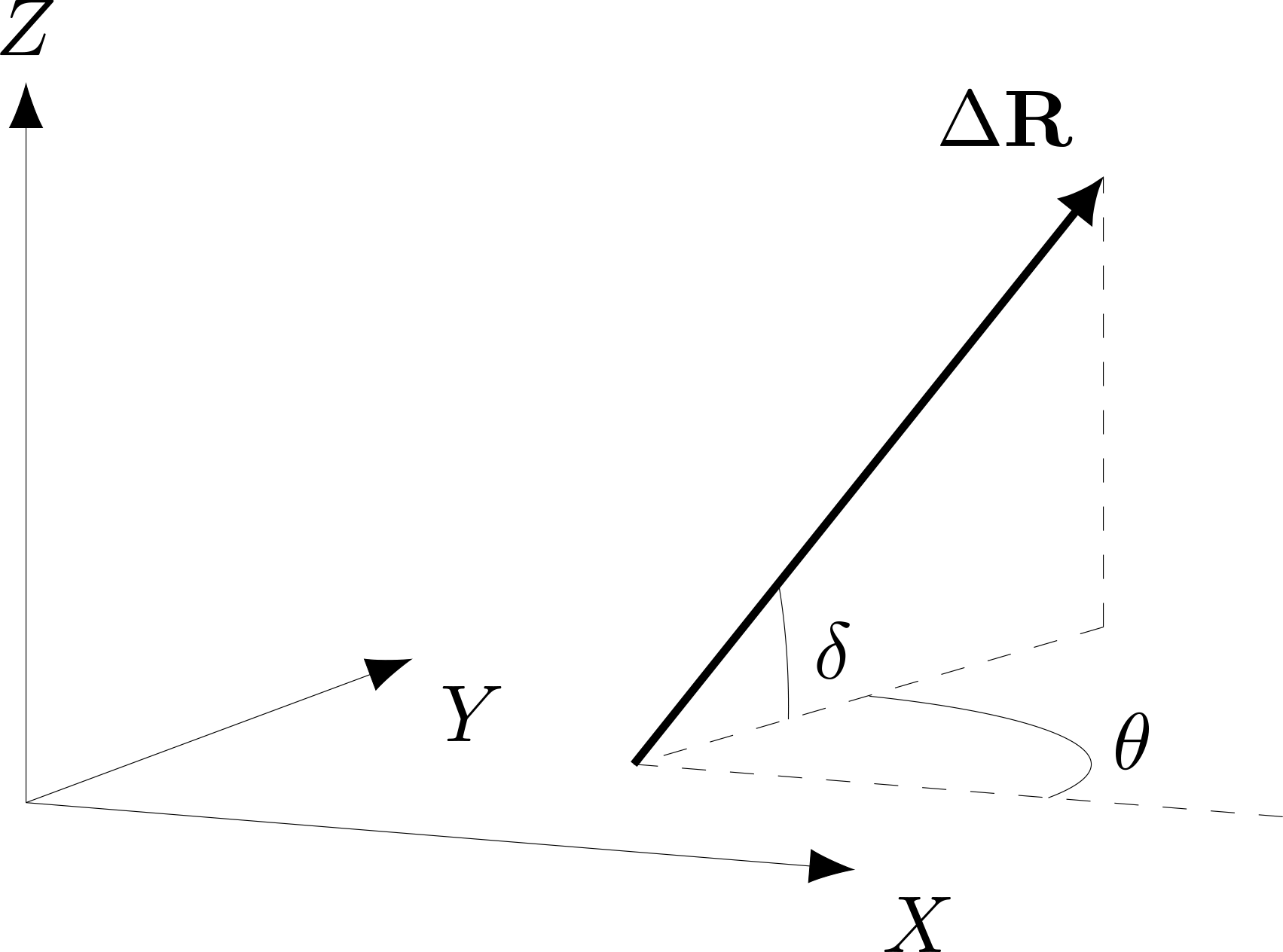
Figure 5The vector ΔR and its orientation in the state space XYZ, characterizing the stress perturbation imposed on the system by earthquakes produced by neighbouring faults.
Since the stress perturbation does not alter the friction coefficients of rocks, it is reasonable to assume that the ratio ϵ between dynamic and static friction is unchanged on both asperities. Therefore, letting and be the new dynamic frictions on asperity 1 and 2, respectively, we have
The consequent changes in dynamic frictions are ϵΔβ1 and ϵΔβ2 on asperity 1 and 2, respectively.
4.1 Effects of the perturbation
The stress transfer resulting from earthquakes on neighbouring faults alters several parameters of the model. A first remarkable change concerns the strength of the asperities. After the perturbation, we can define a new ratio
which differs from the original value of β given in Eq. (1). Moreover, the stress transfer may be so intense that the weaker asperity may become the stronger one: that is, it may result in .
The variations in static frictions entail different conditions for the onset of motion of the asperities. Taking Eq. (22) into account, Eqs. (7) and (8) become, respectively,
By combination with Eq. (2), these conditions define the planes
that we call and , respectively. Conversely, the planes Γ1 and Γ2 are not affected by the stress perturbation, since they do not depend on frictions. We conclude that changes in normal stress modify the sticking region of the system, describing a new hexahedron H′ in the state space. The coordinates of its vertices are
The volume of H′ is : thus, the set of states corresponding to stationary asperities is enlarged or reduced, depending on how normal stresses on the asperities are modified.
Following the changes in static frictions, the surface Σ in Eq. (10) is replaced by a new surface Σ′ expressed by
where
As a result, the sticking region H′ is split in two subsets and ; furthermore, its faces and are divided into subsets , and , , respectively.
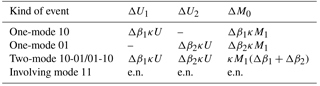
As a consequence of the changes in dynamic frictions, the amount of slip that asperities undergo during a seismic event is modified. In turn, the perturbation alters the seismic moment associated with an earthquake. The variations in the final slip amplitudes U1 and U2 of asperity 1 and asperity 2, respectively, and in the final seismic moment M0 associated with the different seismic events predicted by the model are listed in Table 2.
4.1.1 Changes in Coulomb forces
The variations in tangential stresses and static frictions discussed so far entail a change in the Coulomb forces assigned to the asperities. Combining Eq. (5) with Eqs. (19) and (19), these changes are given by
or, exploiting Eqs. (22) and (22),
The sign of determines whether the perturbation brings an asperity closer to or farther from the failure; specifically, positive variations entail that slip is favoured, and vice versa. Equations (29) and (29) clearly point out that this effect is regulated by the orientation of the vector ΔR in the state space. Bearing in mind the observations made in Sect. 2, we find that is at its maximum when ΔR is perpendicular to plane Π1 and points toward it; it vanishes when ΔR is parallel to plane Π1, and it is at its minimum when ΔR is perpendicular to plane Π1 and points away from it. Analogous considerations can be made for .
On the whole, the effect of the stress perturbation can be discussed in terms of the quantity
Let us assume that the system is at a certain state before the perturbation; accordingly, the next seismic event on the fault will start with the failure of asperity 1. If ΔFC>0, the perturbation favours the slip of asperity 2 more than the slip of asperity 1: therefore, the system is brought to a state closer to the condition for the simultaneous failure of the asperities and thus to the Σ surface. On the contrary, perturbations for which ΔFC<0 take the system farther from the Σ surface. The opposite holds for an unperturbed state .
Table 2Changes in the final slip amplitudes U1 and U2 of asperity 1 and 2 and in the seismic moment M0 associated with the different seismic events predicted by the model, after a stress perturbation from neighbouring faults. The entry e.n. is the abbreviation for evaluated numerically.
4.1.2 Changes in the duration of the inter-seismic interval
As already stated, stress perturbations can anticipate or delay the occurrence of an earthquake produced by a certain asperity. We now quantify this effect in terms of the variation in the duration of the inter-seismic interval. Generally speaking, the perturbation vector ΔR may cross the Σ surface and thus bring the system from an unperturbed state within H1 (H2) to a perturbed state within (). For the sake of simplicity, we consider here only the particular case in which the perturbation vector ΔR does not cross the Σ surface. An example of a more general case will be shown in Sect. 5 for a real fault.
Let us first focus on the case in which the unperturbed state . The time required by the orbit of the system to reach plane Π1, triggering the failure of asperity 1, was calculated by Amendola and Dragoni (2013) as
with γ1 given in Eq. (11). If the stress perturbation brings the system to a state and the static friction on asperity 1 to β1, the time required by the orbit to reach plane is
with given in Eq. (28). The difference between the two times is
where Eq. (29) has been employed.
If instead , the time required by the orbit of the system to reach plane Π2, triggering the failure of asperity 2, is given by (Amendola and Dragoni, 2013)
with γ2 given in Eq. (11). If the stress perturbation takes the system to a state and the static friction on asperity 2 to β2, the time required to reach plane is
with given in Eq. (28). The difference between the two times is
where Eq. (29) has been employed. Positive values of ΔT1 and ΔT2 correspond to a delay in the occurrence of an earthquake on asperity 1 and 2, respectively, and vice versa.
4.1.3 Discussion
According to the model, rock rheology plays a critical role in the response to stress perturbations. In the case of purely elastic coupling between the asperities, Dragoni and Piombo (2015) showed that the changes in the duration of the inter-seismic interval prior to the failure of asperity 1 and 2 are, respectively,
Accordingly, an increase in the Coulomb force associated with a given asperity () directly yields the anticipation of the slip of that asperity, and vice versa. What is more, the variation in the duration of the inter-seismic interval is proportional to the change in the Coulomb force associated with the asperity.
Conversely, in the viscoelastic case there is no straightforward connection between the sign of and the anticipation or delay of an earthquake on the associated asperity. In fact, the expressions (31) and (34) obtained for ΔT1 and ΔT2 in the previous section indicate that the net effect depends in a non-trivial way on the particular state of the fault at the time of the stress perturbation and right after it. This result points out the complex interplay between the post-seismic evolution of a fault in the presence of viscoelastic relaxation and the stress transfer from neighbouring faults.
We study the effects of the 16 October 1999 Mw 7.1 Hector Mine, California, earthquake on the post-seismic evolution of the fault that generated the 28 June 1992 Mw 7.3 Landers, California, earthquake. The geometry of the two faults is shown in Fig. 6.
The 1992 Landers earthquake was a right-lateral strike-slip event that can be approximated as the result of the slip of two coplanar asperities (Kanamori et al., 1992): a northern one (asperity 1) and a southern one (asperity 2), with average slips u1=6 m and u2=3 m, respectively. Following Dragoni and Tallarico (2016), we assume a common area A=300 km2 for both the asperities. We place the centres of asperity 1 and asperity 2 at 34.46∘ N, 116.52∘ W and 34.20∘ N, 116.44∘ W, respectively, with a common depth of 8 km. The earthquake started with the failure of asperity 2, followed by the failure of asperity 1. We characterize the event by strike, dip and rake angles of 345, 85 and 180∘, respectively, an average of the values provided by Kanamori et al. (1992) for the two phases of the earthquake.
The 1992 event was followed by remarkable post-seismic deformation, which can be interpreted as the result of several processes. For the sake of the present application, we assume viscoelastic relaxation as the most significant mechanism. We assign a viscosity to the lower crust at Landers, averaging the estimates provided by Deng et al. (1998), Pollitz et al. (2000), Freed and Lin (2001) and Masterlark and Wang (2002). With a rigidity μ=30 GPa, the corresponding Maxwell relaxation time is .
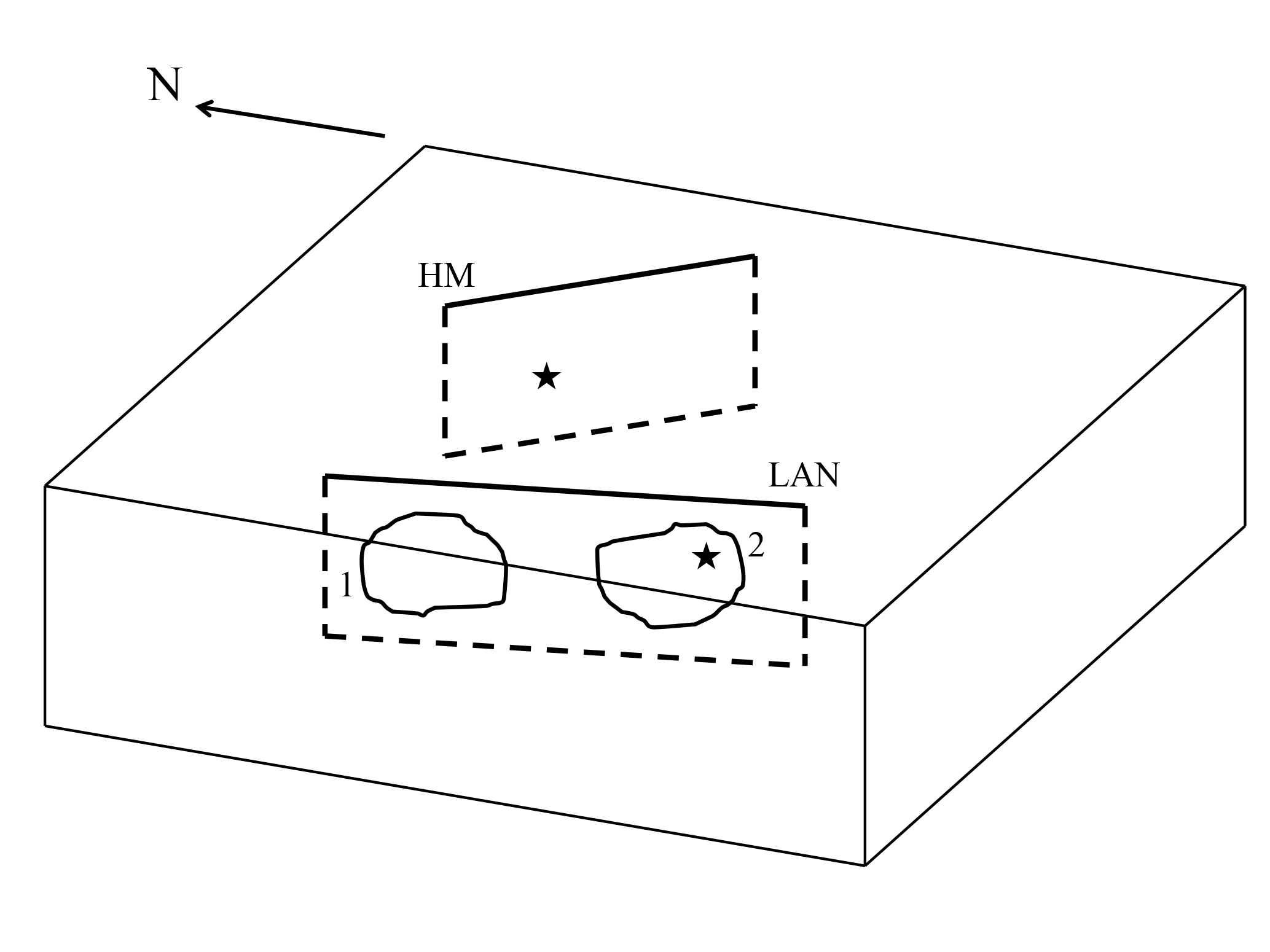
Figure 6Geometry of the Landers (LAN) and Hector Mine (HM), California, faults that generated the 1992 and 1999 earthquakes, respectively. The stars indicate the hypocentres of the seismic events. The labels 1 and 2 identify the asperities on the Landers fault.
We model the 1992 earthquake as a two-mode event 01-10 starting from mode 00. Accordingly, the orbit of the system during mode 00 lies inside the subset H2 of the sticking region and the state P1 at the beginning of the earthquake belongs to segment s2 (Fig. 4). The coordinates of P1 are
with
where the extreme values Za and Zb correspond to the end points of s2:
At the end of mode 01, the system is at point P2 with coordinates
where mode 10 starts. As Z1 varies in the interval given in Eq. (37), an infinite number of points P2 describe a segment r2 on the subset Q1 of the face AECD and parallel to the edge CD. Mode 10 terminates at point P3 with coordinates
Again, as Z1 varies in the interval given in Eq. (37), there is an infinite number of points P3 defining another segment q2 parallel to the edge CD. This segment is situated within the sticking region and crosses the surface Σ for Z1=Zc, with .
Dragoni and Tallarico (2016) studied the 1992 Landers earthquake under the hypothesis of purely elastic coupling between the asperities. Following the authors, we take α=0.1, β=0.5, γ=1.5 and ϵ=0.7, a set of values yielding modelled moment rate and seismic spectrum comparable with the observations. Thus, we have U≃0.546 and κ≃0.52. As for viscoelastic relaxation, it can be characterized by the product VΘ (Amendola and Dragoni, 2013), which can be estimated as
where v=3 cm a−1 is the relative plate velocity at Landers (Wallace, 1990). Accordingly, we have VΘ≃0.007.
Every state P1 on segment s2, where the 1992 earthquake began, corresponds to a specific state P3 on segment q2, where the 1992 earthquake ended. Exploiting Eq. (39), we can express the coordinates (40) of P3 as a function of Z1. Since q2 crosses the surface Σ, the state P3 can belong to H1,H2 or Σ, in correspondence to , and Z1=Zc, respectively. In the first case, the next event will start with the failure of asperity 1; in the second case, with the failure of asperity 2; in the third case, with the simultaneous failure of the asperities. With the values of α, β, κ and U listed above, we find , Zb≃3.58 and Zc≃0.78. Accordingly, only about one-quarter of segment q2 lies inside the subset H1 of the sticking region. Without any further discussion and neglecting the stress perturbation caused by the Hector Mine earthquake, we would infer that future events on the 1992 fault are more likely to start with the failure of asperity 2.
5.1 Stress perturbation by the 1999 Hector Mine earthquake
The 1999 Hector Mine earthquake was generated by right-lateral strike-slip faulting located at 34.59∘ N, 116.27∘ W, about 20 km north-east from the Landers fault (Jónsson et al., 2002; Salichon et al., 2004). We characterize the event averaging the data available in the SRCMOD database and assume strike, dip and rake angles of 330, 80 and 180∘, respectively; a depth of 10 km; and a seismic moment of 6.62×10¹⁹ Nm.
The stress transferred to the asperities at Landers can be evaluated employing the model of Appendix Appendix A, taking
As a result, the normal and tangential components of the perturbing stress on asperity 1 are
Accordingly, the static friction on asperity 1 is reduced and right-lateral slip is favoured. As for asperity 2, the components of the perturbing stress are
suggesting that static friction on asperity 2 is reduced and right-lateral slip is inhibited.
We now introduce the effect of the perturbation in the framework of the discrete model. The changes in the tangential forces (2) on the asperities are
The static friction fs1 on asperity 1 can be evaluated as (Dragoni and Santini, 2012)
where the constant
is an expression of the coupling between the asperities and the tectonic plates. With d=80 km (Masterlark and Wang, 2002), it results in MPa. Hence, we have
From Eqs. (19)–(19), the components of the perturbation vector ΔR are
As a result, the orientation of ΔR in the state space is characterized by angles rad and rad. The changes in static frictions (23) can be calculated as
where ks is the effective static friction coefficient on asperity 1. Assuming ks=0.4, we get
Finally, from Eqs. (29) and (29), the changes in Coulomb forces on the asperities are
At the time of the Hector Mine earthquake, the Landers fault was at a state P4 resulting from the post-seismic evolution of any of the possible states P3∈q2 where the 1992 event ended. The coordinates of P4 can be calculated from the solution to the equations of mode 00 given by Dragoni and Lorenzano (2015) and taking into account that the time interval elapsed between the 1992 Landers and 1999 Hector Mine earthquakes amounts to about 7.3 years:
where
Making use of Eqs. (39) and (40), we can express the coordinates of P4 as a function of . Accordingly, there is an infinite number of points P4 defining a vector t2 inside the sticking region. At , the perturbation vector ΔR moves every state P4 to a new state with coordinates
which can be expressed as a function of . As a result, a new vector identifies the state of the Landers fault after the Hector Mine earthquake.
In order to characterize the effect of the perturbation, let us consider the difference ΔFC defined in Eq. (29): from Eq. (51), we get . Since ΔFC<0, we conclude that the stress perturbation is such that states P4∈H1 are moved to , the state P4∈Σ enters , states P4∈H2 are shifted towards the Σ surface and some of them enter . Specifically, we find that belongs to , and Σ′ in correspondence to , and , with . On the whole, we can draw the preliminary conclusion that the stress perturbation is such that future events on the Landers fault starting with the slip of asperity 1 are favoured over events starting with the slip of asperity 2. A deeper discussion is provided in the following.
5.2 Constraints due to the seismic history to date
In order to improve our knowledge on the state that gave rise to the 1992 Landers earthquake and on the possible future events generated by that fault, we exploit the seismic history between 1999 and the present date. After the perturbation caused by the Hector Mine earthquake, the inter-seismic time of the Landers fault can be calculated from Eq. (30) and Eq. (33) for states belonging to and , respectively:
where
Since no earthquakes have been produced by the Landers fault after the occurrence of the Hector Mine event, up to year 2016, we can exclude the states on the segment s2 yielding an expected inter-seismic time (Eq. 55) shorter than or equal to 17 years. The requirement
is satisfied by states on segment s2 in the subset , with and .
As a consequence, we can constrain the admissible states on the segment
t2. A comparison between the intervals and
points out that more than one-half of the acceptable
subset of t2 belongs to H2. Hence, before the stress
perturbation caused by the Hector Mine earthquake, future events on the 1992
Landers fault were more likely to start with the failure of asperity 2.
In
turn, the refinement of t2 limits the acceptable states on the
segment . From the amplitude of the intervals and , we deduce that the acceptable subset of
is almost equally divided between and
. Therefore, if we consider the influence of the Hector Mine
earthquake on future events generated by the 1992 Landers fault, we conclude
that the stress perturbation yielded homogenization in the probability of
events starting with the failure of asperity 1 or asperity 2. This result is
in agreement with the observation that the perturbation vector ΔR shifted the whole segment t2 towards the subset
of the sticking region.
These conclusions would have to be reconsidered if new stress perturbations from neighbouring faults were to affect the post-seismic evolution of the Landers fault in the future. In addition, if no earthquakes were to be observed for some time on the Landers fault, the refining procedure discussed above could be repeated and the admissible subsets of segments s2, t2 and could be constrained with further precision.
5.3 Effects of the stress perturbation on future earthquakes
Finally, we discuss the features of the next seismic event generated by the 1992 Landers fault, highlighting the changes due to the Hector Mine earthquake.
Every state P1∈s2 where the 1992 earthquake began corresponds to a particular state P4∈t2 and before and after the stress perturbation associated with the Hector Mine earthquake, respectively. Since the segment t2 intersects the surface Σ, the state P4 can belong to H1, H2 or Σ (Fig. 3), thus affecting the asperity that will fail the first at the beginning of the next earthquake on the fault. In the first case, the next event will start with the failure of asperity 1, in the second case with the failure of asperity 2, in the third case with the simultaneous failure of the asperities. Analogous considerations hold for states in and Σ′, respectively.
The number and the sequence of dynamic modes in the earthquake depend on the sub-interval of Z1 considered. The details are summarized in Table 3 for both the unperturbed and perturbed cases. Taking these specifics into account and referring to Tables 1 and 2, we evaluate the seismic moments M0 and associated with the expected future earthquake on the 1992 fault before and after the Hector Mine earthquake, respectively. In Fig. 7, we show the difference
as a function of . Owing to the translation imposed to the segment t2 by the perturbation vector ΔR, the sign of ΔM0 changes across the different sub-intervals of Z1. The energy released by the earthquake is increased for , while it is reduced elsewhere.
Another significant result of the stress perturbation concerns the variation in the inter-seismic time before the next seismic event. As in Sect. 5.2, we consider the post-seismic evolution from 1999 onwards and set the origin of times at the occurrence of the Hector Mine earthquake. The expected inter-seismic time Tis prior to the stress perturbation can be calculated from Eqs. (29) and (32) for states P4 belonging to H1 and H2, respectively:
where
The inter-seismic time after the stress perturbation has been given in Eq. (55). The difference
is shown in Fig. 8 as a function of . For states P4∈H1 corresponding to and states P4∈H2 corresponding to , this difference coincides with Eqs. (31) and (34), respectively.
Table 3Future earthquakes generated by the 1992 Landers, California, fault, as functions of the variable Z1 describing the initial state of the 1992 event, with . The results predicted by the model before and after the stress perturbation associated with the 1999 Hector Mine, California, earthquake are shown. The values and correspond to the largest possible earthquakes before and after the stress perturbation, respectively.
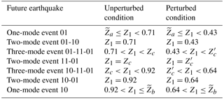
Figure 7Change in the seismic moment released during the next event on the 1992 Landers, California, fault, as a result of the stress perturbation due to the 1999 Hector Mine, California, earthquake. On the horizontal axis, the variable Z1 describing the initial state of the 1992 event. The kinds of seismic event predicted by the model, corresponding to different intervals of Z1, are listed in Table 3. The values Z1=Zc and correspond to the largest possible earthquakes before and after the stress perturbation, respectively.
Some peculiar features stand out. First, we notice that, for all states P4∈H2 corresponding to , that is, for , the inter-seismic time is increased by the stress perturbation, in agreement with the inhibiting effect on asperity 2 suggested by Eq. (51). However, Eq. (51) suggests that the failure of asperity 1 is promoted, but this is not verified by all states , that is, for . In fact, the inter-seismic time is reduced only for , while it is increased for . In the particular case Z1=0.53, there is no change in the inter-seismic time. This is a remarkable result, showing that the presence of viscoelastic relaxation at the time of the stress perturbation entails the unpredictability of the consequent influence in terms of anticipation or delay of future earthquakes, on the basis of the sole knowledge of the change in Coulomb stress.

Figure 8Change in the inter-seismic time before the next event on the 1992 Landers, California, fault, as a result of the stress perturbation due to the 1999 Hector Mine, California, earthquake. On the horizontal axis, the variable Z1 describing the initial state of the 1992 event. The kinds of seismic event predicted by the model, corresponding to different intervals of Z1, are listed in Table 3. The values Z1=Zc and correspond to the largest possible earthquakes before and after the stress perturbation, respectively.
At the occurrence of the next earthquake produced by the Landers fault, the number and sequence of dynamic modes involved and the energy released will reveal more about the state of the system, thus allowing a further refinement of the specific conditions that gave rise to the 1992 event.
We considered a plane fault embedded in a shear zone, subject to a uniform strain rate owing to tectonic loading. The fault is characterized by the presence of two asperities with equal areas and different frictional resistance. The coseismic static stress field due to earthquakes produced by the fault is relaxed by viscoelastic deformation in the asthenosphere.
The fault was treated as a discrete dynamical system with three degrees of freedom: the slip deficits of the asperities and the variation of their difference due to viscoelastic deformation. The dynamics of the system was described in terms of one sticking mode and three slipping modes. In the sticking mode, the orbit of the system lies in a convex hexahedron in the space of the state variables, while the number and the sequence of slipping modes during a seismic event are determined by the particular state of the system at the beginning of the inter-seismic interval preceding the event. The amount of slip of the asperities and the energy released during an earthquake generated by the fault can be predicted accordingly.
The effect of stress transfer due to earthquakes on neighbouring faults was studied in terms of a perturbation vector yielding changes to the state of the system, its sticking region and the energy released during a subsequent seismic event. The specific effect on the evolution of the fault is related with the orientation of this vector in the state space.
We investigated the interplay between the ongoing viscoelastic relaxation on the fault and a stress perturbation imposed during an inter-seismic interval. Following a stress perturbation due to earthquakes on neighbouring faults, an increase in the Coulomb stress associated with a given asperity directly yields the anticipation of the slip of that asperity, and vice versa, if a purely elastic rheology is assumed for the receiving fault (Dragoni and Piombo, 2015). According to the present model, this property no longer holds if the change in Coulomb stress occurs while viscoelastic relaxation is taking place on the receiving fault. In fact, even if the change in the inter-seismic intervals of the asperities can still be evaluated from a theoretical point of view, the specific effect of the stress perturbation could be univocally inferred only if the particular states of the fault at the time of the stress perturbation and right after it were known. The information on the change in Coulomb stress on the fault do not suffice any more.
We applied the model to the stress perturbation imposed by the 1999 Hector Mine, California, earthquake to the fault that caused the 1992 Landers, California, earthquake, which was due to the failure of two asperities and was followed by significant viscoelastic relaxation. We modelled the 1992 Landers earthquake as a two-mode event associated with the separate slip of the asperities and showed how the event is compatible with a number of possible initial states of the fault, which can be screened on the basis of the seismic history to date. The details of the stress transfer associated with the 1999 Hector Mine earthquake were calculated using the relative positions and faulting styles of the two faults as a starting point. We discussed the effect of the stress perturbation, pointing out the complexity of its influence on the possible future events generated by the 1992 Landers fault in terms of the associated energy release, the sequence of dynamic modes involved and the duration of the inter-seismic interval. Specifically, we showed that the consequences of the 1999 Hector Mine earthquake on the post-seismic evolution of the 1992 Landers fault depend on the specific state of the Landers fault at the time of the 1999 earthquake and immediately after it, even if the variations in the Coulomb stress on the asperities at Landers are known. On the whole, the application allowed the exemplification of the critical unpredictability of the effect of a stress perturbation occurring while viscoelastic relaxation is taking place.
Another source of complication may be represented by the interaction between viscoelastic relaxation and stable creep on the fault. This problem is beyond the scope of the present work, but it may be object of future research by combining elements of the present model with the one of Dragoni and Lorenzano (2017).
All data and results supporting this work were gathered from the papers listed in the References and are freely available to the public. Specifically, data on the 1999 Hector Mine, California, earthquake were collected from the Finite-Source Rupture Model Database (SRCMOD) available at http://equake-rc.info/SRCMOD/. The website was last accessed on December 2016.
We consider two plane faults, namely fault 1 and fault 2, embedded in an infinite, homogeneous and isotropic Poisson medium of rigidity μ (Fig. A1). Following the slip of fault 1 (perturbing fault), stress is transferred to fault 2 (receiving fault). We calculate the normal traction σn and the tangential traction in the direction of slip σt transferred to the receiving fault, estimated as the average value at its centre.
We define a coordinate system with axes corresponding with the directions of dip, strike and normal on fault 1, respectively. Fault 1 lies on the plane z=0 and its centre is in the origin of the coordinate system. Accordingly, the unit vector perpendicular to fault 1 is . We call ϕ1, ψ1 and λ1 the strike, dip and rake angles of fault 1, respectively. The slip direction of fault 1 is then given by
Fault 2 is characterized by strike and dip angles ϕ2 and ψ2, respectively. Accordingly, the unit vector perpendicular to fault 2 is given by
where
Let λ2 be the preferred rake angle on fault 2, correlated with the orientation of tectonic loading: λ2=0∘ for left-lateral strike slip, λ2=180∘ for right-lateral strike slip, ∘ for normal dip slip and λ2=90∘ for reverse dip slip. The corresponding slip direction is
We name (Ei,Ni) and Di the UTM (Universal Transverse Mercator) coordinates and depths of the centres of the faults, respectively. In our reference system, the coordinates of the centre of fault 2 are identified by the following three steps:
-
placing the origin at the centre of fault 1:
-
clockwise rotation about the z axis by the angle ϕ1:
-
counterclockwise rotation about the y axis by the angle ψ1:
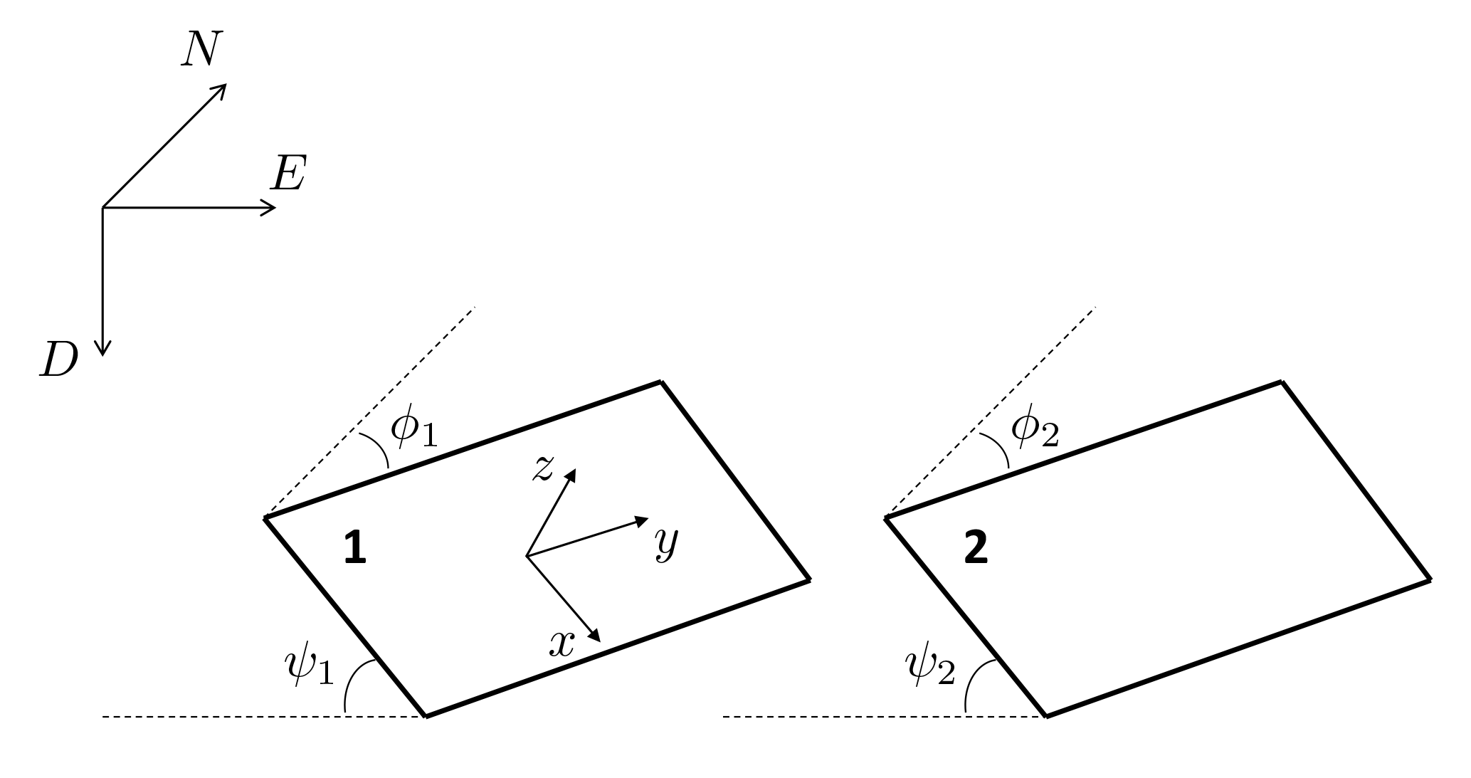
Figure A1Geometry of the model employed to study the stress transfer between neighbouring faults. Fault 1 is the perturbing fault, while fault 2 is the receiving fault. The coordinates are the UTM coordinates and depth of the centres of the faults, respectively, whereas the axes correspond with the directions of dip, strike and normal on fault 1, respectively. The angles ϕ and ψ are the strike and dip angles of the faults, respectively.
The perturbing fault is treated as a point-like dislocation source (a double couple of forces) located at the origin. This is a good approximation for non-overlapping regions (Dragoni and Lorenzano, 2016). Let m0 be the scalar seismic moment of the dislocation. The ith component of the static displacement field generated by the slip of fault 1 is
where Mij is the moment tensor associated with the dislocation source
and Gij is the Somigliana tensor
with
The components of the stress field are given by
where eij is the strain field associated with the displacement field (A5). Finally, the normal traction σn and the tangential traction in the direction of slip σt on fault 2 are
The signs of σn and σt define the effect of the stress transfer on fault 2. If σn>0, the amount of compressional stress on the receiving fault is reduced, and vice versa. If σt>0, the slip of the receiving fault is promoted, and vice versa.
EL developed the model, produced the figures and wrote a preliminary version of the paper; MD checked the equations and revised the text. Both authors discussed the results extensively.
The authors declare that they have no conflict of interest.
The authors are thankful to the editor Richard Gloaguen, to Sylvain Barbot and to an anonymous referee for their useful
comments on the first version of the paper.
Edited by: Richard Gloaguen
Reviewed by: one anonymous referee
Amendola, A. and Dragoni, M.: Dynamics of a two-fault system with viscoelastic coupling, Nonlin. Processes Geophys., 20, 1–10, https://doi.org/10.5194/npg-20-1-2013, 2013.
Christensen, D. H. and Beck, S. L.: The rupture process and tectonic implications of the great 1964 Prince William Sound earthquake, Pure Appl. Geophys., 142, 29–53, 1994.
Delouis, B., Nocquet, J. M., and Vallée, M.: Slip distribution of the February 27, 2010 Mw = 8.8 Maule earthquake, central Chile, from static and high-rate GPS, InSAR, and broadband teleseismic data, Geophys. Res. Lett., 37, L17305, https://doi.org/10.1029/2010GL043899, 2010.
Deng, J., Gurnis, M., Kanamori, H., and Hauksson, E.: Viscoelastic flow in the lower crust after the 1992 Landers, California, earthquake, Science, 282, 1689–1692, 1998.
Dragoni, M. and Lorenzano, E.: Stress states and moment rates of a two-asperity fault in the presence of viscoelastic relaxation, Nonlin. Processes Geophys., 22, 349–359, https://doi.org/10.5194/npg-22-349-2015, 2015.
Dragoni, M. and Lorenzano, E.: Conditions for the occurrence of seismic sequences in a fault system, Nonlin. Processes Geophys., 23, 419–433, https://doi.org/10.5194/npg-23-419-2016, 2016.
Dragoni, M. and Lorenzano, E.: Dynamics of a fault model with two mechanically different regions, Earth Planets Space, 69, 145, https://doi.org/10.1186/s40623-017-0731-2, 2017.
Dragoni, M. and Piombo, A.: Effect of stress perturbations on the dynamics of a complex fault, Pure Appl. Geophys., 172, 2571–2583, 2015.
Dragoni, M. and Santini, S.: Long-term dynamics of a fault with two asperities of different strengths, Geophys. J. Int., 191, 1457–1467, 2012.
Dragoni, M. and Santini, S.: A two-asperity fault model with wave radiation, Phys. Earth. Planet. In., 248, 83–93, 2015.
Dragoni, M. and Tallarico, A.: Complex events in a fault model with interacting asperities, Phys. Earth Planet. In., 257, 115–127, 2016.
Freed, M. and Lin, J.: Delayed triggering of the 1999 Hector Mine earthquake by viscoelastic stress transfer, Nature, 411, 180–183, 2001.
Harris, R. A.: Introduction to special section: Stress triggers, stress shadows, and implications for seismic hazard, J. Geophys. Res.-Sol. Ea., 103, 24347–24358, 1998.
Jónsson, S., Zebker, H., Segall, P., and Amelung, F.: Fault slip distribution of the 1999 Mw 7.1 Hector Mine, California, earthquake, estimated from satellite radar and GPS measurements, B. Seismol. Soc. Am., 92, 1377–1389, 2002.
Kanamori, H., Thio, H., Dreger, D., Hauksson, E., and Heaton, T.: Initial investigation of the Landers, California, Earthquake of 28 June 1992 using TERRAscope, Geophys. Res. Lett., 19, 2267–2270, 1992.
Lay, T., Kanamori, H., and Ruff, L.: The asperity model and the nature of large subduction zone earthquakes, Earthquake Pred. Res., 1, 3–71, 1982.
Masterlark, T. and Wang, H. F.: Transient stress-coupling between the 1992 Landers and 1999 Hector Mine, California, earthquakes, B. Seismol. Soc. Am., 92, 1470–1486, 2002.
Pollitz, F. F., Peltzer, G., and Bürgmann, R.: Mobility of continental mantle: Evidence from postseismic geodetic observations following the 1992 Landers earthquake, J. Geophys. Res.-Sol. Ea., 105, 8035–8054, 2000.
Ruff, L. J.: Asperity distributions and large earthquake occurrence in subduction zones, Tectonophysics, 211, 61–83, 1992.
Salichon, J., Lundgren, P., Delouis, B., and Giardini, D.: Slip history of the 16 October 1999 Mw 7.1 Hector Mine earthquake (California) from the inversion of InSAR, GPS, and teleseismic data, B. Seismol. Soc. Am., 94, 2015–2027, 2004.
Scholz, C. H.: The Mechanics of Earthquakes and Faulting, 2nd ed., Cambridge University Press, Cambridge, UK, 2002.
Steacy, S., Gomberg, J., and Cocco, M.: Introduction to special section: Stress transfer, earthquake triggering, and time-dependent seismic hazard, J. Geophys. Res.-Sol. Ea., 110, B05S01, https://doi.org/10.1029/2005JB003692, 2005.
Stein, R. S.: The role of stress transfer in earthquake occurrence, Nature, 402, 605–609, 1999.
Turcotte, D. L.: Fractals and Chaos in Geology and Geophysics, 2nd ed., Cambridge University Press, Cambridge, UK, 1997.
Twardzik, C., Madariaga, R., Das, S., and Custódio, S.: Robust features of the source process for the 2004 Parkfield, California, earthquake from strong-motion seismograms, Geophys. J. Int., 191, 1245–1254, 2012.
Wallace, R. E.: The San Andreas fault system, California, U.S. Geol. Surv. Prof. Pap., 1515, 189–205, 1990.
- Abstract
- Introduction
- The model
- Dynamic modes and slip in a seismic event
- Stress perturbations from neighbouring faults
- An application: perturbation of the 1992 Landers fault by the 1999 Hector Mine earthquake
- Conclusions
- Data availability
- Appendix A: Estimate of the stress perturbation
- Author contributions
- Competing interests
- Acknowledgements
- References