the Creative Commons Attribution 4.0 License.
the Creative Commons Attribution 4.0 License.
 | 22 Mar 2018
Complex network description of the ionosphere
Shikun Lu
Hao Zhang
Yihong Li
Chao Niu
Xiaoyun Yang
Daizhi Liu
Complex networks have emerged as an essential approach of geoscience to generate novel insights into the nature of geophysical systems. To investigate the dynamic processes in the ionosphere, a directed complex network is constructed, based on a probabilistic graph of the vertical total electron content (VTEC) from 2012. The results of the power-law hypothesis test show that both the out-degree and in-degree distribution of the ionospheric network are not scale-free. Thus, the distribution of the interactions in the ionosphere is homogenous. None of the geospatial positions play an eminently important role in the propagation of the dynamic ionospheric processes. The spatial analysis of the ionospheric network shows that the interconnections principally exist between adjacent geographical locations, indicating that the propagation of the dynamic processes primarily depends on the geospatial distance in the ionosphere. Moreover, the joint distribution of the edge distances with respect to longitude and latitude directions shows that the dynamic processes travel further along the longitude than along the latitude in the ionosphere. The analysis of “small-world-ness” indicates that the ionospheric network possesses the small-world property, which can make the ionosphere stable and efficient in the propagation of dynamic processes.
- Article
(4009 KB) - Full-text XML
- BibTeX
- EndNote


Including large numbers of irregularities with different sizes and affected by various factors (like solar irradiation, geomagnetic field, gravity wave and tidal wave; Kelly, 2009), the ionosphere performs as a complex system in terms of the spatial and temporal variation. A complex network is an efficient tool to study the characteristics of complex systems that contain a large number of interacting parts. Its application spans various scientific fields (Zerenner et al., 2014), such as biology (e.g., protein interaction networks), information technology (e.g., World Wide Web) and social sciences (e.g., social networks; Wang et al., 2016a, b). The application of complex network theory to ionosphere science is still a young field, since few research studies have been reported. The network theory was discussed by Podolská et al. with two abstracts in the 2010 and 2012 EGU General Assembly Conference (Podolská et al., 2010, 2012). The aim of the first abstract was to examine the influence of geomagnetic disturbances and solar activity on thermal plasma parameters. The other abstract was focused on an attempt to find out time shifts between fundamental ionospheric parameters. Therefore, none of them tried to describe the global ionosphere based on a complex network.
In modern statistical mechanics of geophysics, especially seismological science, the idea of complex networks is receiving significant attention. Baiesi and Paczuski (2005) constructed directed networks of earthquakes by placing a link between pairs of events that were strongly correlated. Their results showed that the network was scale-free and highly clustered. Abe and Suzuki (2006) constructed growing random networks by adding an edge between two successive earthquakes and found that these earthquake networks were scale-free and small-world. The constructions of the above two networks were based on the expert judgment of adding an edge and ignored the uncertainty in the system. Jiménez et al. (2008) divided the southern California region into cells of 0.1∘ and calculated the correlation of activities among them to create networks, which showed the small-world features. Suteanu (2014) proposed a network-based method for the assessment of earthquakes' relationships in space–time–magnitude patterns and further applied the results for the study of temporal variations in volcanic seismicity patterns. Those two networks were built based on correlation, which was a linear measurement of the interactions in the objective system.
Another geophysical application of complex networks is in climate science (Nocke et al., 2015). Peron et al. (2014) also built a temperature network by correlation and regarded the global grid points as nodes. They showed that the network characteristics of the North American region marked the differences between the eastern and western regions. Such differences can be viewed as a reflection of the presence of a large network community on the west side of the continent. To depict the nonlinearity and uncertainty in the climate, information theory is introduced to construct the complex network of climate. Donges et al. (2009a, b) used complex networks to uncover a backbone structure carrying matter and energy in the global surface air temperature field. They used mutual information (MI) to construct the network, which was undirected because the mutual information was symmetric, in order to measure the dynamical similarity of surface air temperature between regions. Hlinka et al. (2013) investigated the reliability of directed climate networks being built by conditional mutual information (CMI), using dimensionality-reduced surface air temperature data. Compared with MI, CMI is asymmetric and able to build directed networks for global surface air temperature. However, both MI and CMI are standard bivariate methods, which only describe the interactions between two spatial points without considering the influence of the others. The same is true of the correlation. A probabilistic graph is an efficient method to describe the nonlinear interactions within the system from a holistic perspective (Koller and Friedman, 2009). Furthermore, similar to seismology and climate science, the ionosphere is also distributed geographically. The ionospheric variation involves spatial interactions and flows. These research studies propose a possibility that approaches from the perspective of complex networks may also shed new light on ionospheric features. In this article, a probabilistic graph is employed to model the dynamic processes within the ionosphere and build the ionospheric complex network.
Within the global ionosphere, there are interactions among the variations over different positions. Variations over one position may cause variations over other positions. The motivation of the current study is to explore the causal interactions between the vertical total electron content (VTEC) over different positions or cells of a global ionosphere map (GIM) within the global ionosphere based on the directed complex network. Hence, we can have a deep understanding of the dynamic processes within the ionosphere. We interpret the dynamic ionospheric processes as the information flow in the directed network and explore the ionospheric characteristics on a global scale. The VTEC dataset supplied by the Centre for Orbit Determination in Europe (CODE) in 2012 is selected.
The article is organized as follows. The data and method description are provided in Sect. 2. Furthermore, the results about the patterns of the ionospheric interactions are presented in Sect. 3. The scale-free topology of the ionospheric network is checked by conducting a power-law hypothesis test. The distribution of the edge distances is calculated to analyze the propagation of the dynamic processes in the ionosphere. The small-world structure of the ionospheric network is explored to examine the stability of the ionosphere. Section 4 discusses the summaries and conclusions.
2.1 VTEC data source
As a critical physical quantity of the ionosphere, VTEC carries abundant information about the variations of the ionosphere (Ercha et al., 2015). The International Global Navigation Satellite System Service (IGS) supplies global VTEC data with 2 h time resolution. The dataset is determined from more than 200 IGS stations on a global scale (Wei et al., 2009). CODE, as one of the analysis centers of IGS, has estimated VTEC from the dual-frequency code and phase data of GPS since April 1998 (Guo et al., 2015). In the current research, VTEC data are derived from CODE (ftp://ftp.aiub.unibe.ch/CODE/) in the form of a GIM. The GIM ranges from −180 to 180∘ along the longitude and from −87.5 to 87.5∘ along the latitude. The negative values stand for the south latitude and west longitude. The size of an elementary GIM cell is 5∘ along the longitude and 2.5∘ along the latitude. Each GIM cell is defined as a variable, which is a node in the ionospheric network. The VTEC data over the GIM cells are the observations. For the decrease of the computation by reducing the variables' quantity, the size of the GIM cells has been doubled. Therefore, the latitude and longitude of GIM cells become 5 and 10∘. The number of variables (GIM cells) is 36×36, which is 1296, because 180 and are the same for longitude. In this paper, we select the data from 2012.
2.2 Mapping the data to a complex network
As a complex system, the ionosphere is usually characterized by the presence of multiple interrelated aspects, which are spatially distributed. Affected by various factors, the ionosphere also involves a significant amount of uncertainty. Moreover, our observations are always noisy; even observed aspects are often measured with some error. Thus, probability needs to be used to represent such random properties. Furthermore, a probabilistic graph can efficiently describe the nonlinearity within the system from a holistic perspective (Koller and Friedman, 2009). As a result, a probabilistic graph is selected to model the interrelation and uncertainty in the ionosphere. We describe the GIM data as the realization of a multivariate probabilistic graph on the global spatial grid.
Probabilistic graphs use a graph-based representation as the basis for compactly encoding a complex probabilistic distribution over a high-dimensional space (Koller and Friedman, 2009). A probabilistic graph is a useful way of visualizing interactions between multiple variables. Therefore, in addition to inference, probabilistic graphs can also be used to discover the knowledge within the dataset. As a kind of complex network, probabilistic graphs are constructed to represent a joint distribution by making conditional independence (CI) assumptions. The nodes in the networks represent variables, and the edges represent CI assumptions (Murphy, 2012). The absence of an edge between two nodes implies that the corresponding variables are conditionally independent given all other nodes. Based on the probability theory, we say variables X and Y are CI if the conditional joint distribution can be written as a product of conditional marginal:
In our study, X and Y are the two given GIM cells and Z represents the GIM cells except X and Y. Thus, the analysis is performed from a holistic perspective. As suggested in Zerenner et al. (2014), a directed complex network can offer additional knowledge, like the distinction between child and parent nodes. Thus, we construct the ionospheric networks that only include directed edges between GIM cells. Suppose two GIM cells are not directly connected (conditionally independent) within the ionospheric network, there should be no interactions between these cells after eliminating all of the existing edges. The directed edges here represent the causal interactions. In other words, after the variations of VTEC over a certain GIM cell, there are some related variations appearing over other GIM cells. In the following, the construction of the directed ionospheric network (also known as a Bayesian probabilistic graph or Bayesian network) is introduced to describe the dynamic processes in the global ionosphere. Dynamic processes are constituted by a series of causal interactions among the GIM cells. Conditional independence tests involving sets of variables can be used to determine the existence and direction of edges (Ebert-Uphoff and Deng, 2012).
The cells in the GIMs are defined as the variables of VTEC distributed throughout the globe. As the nodes on the network, the variables are separated by their own geospatial locations. The VTEC of each variable is arranged in the form of a time series with 2 h time resolution. Thus, for the year 2012, the length of the observations is 4392 (). We employ a structure learning algorithm for Bayesian networks as a basis for the construction of the ionospheric networks. In our study, the measurements of the 1296 variables are all continuous. To build the directed network, we should determine the existence and directions of edges between any two variables from a holistic perspective instead of just considering the two. The Fast Greedy Equivalence Search (FGS) algorithm proposed by Ramsey et al. (2017) works well for large numbers of continuous variables to build Bayesian networks. This algorithm utilizes the strategy that edges are iteratively added starting with an empty network, according to maximal increases in the Bayesian information criterion (BIC) score (Schwarz, 1978). Here, the variables' distributions are assumed to be Gaussian. We use the implementation of the FGS algorithm in the TETRAD package (Version 5.3.0-2, available at http://www.phil.cmu.edu/projects/tetrad/, last access: 22 March 2018) and make the penalty discount 10. TETRAD possesses a convenient user interface to enter preknowledge. As the ionospheric network includes 1296 nodes and 10 985 directed edges in the globe, it is hard to fully present such a complex network. Here, we exhibit part of the ionospheric network. The result is shown in Fig. 1.
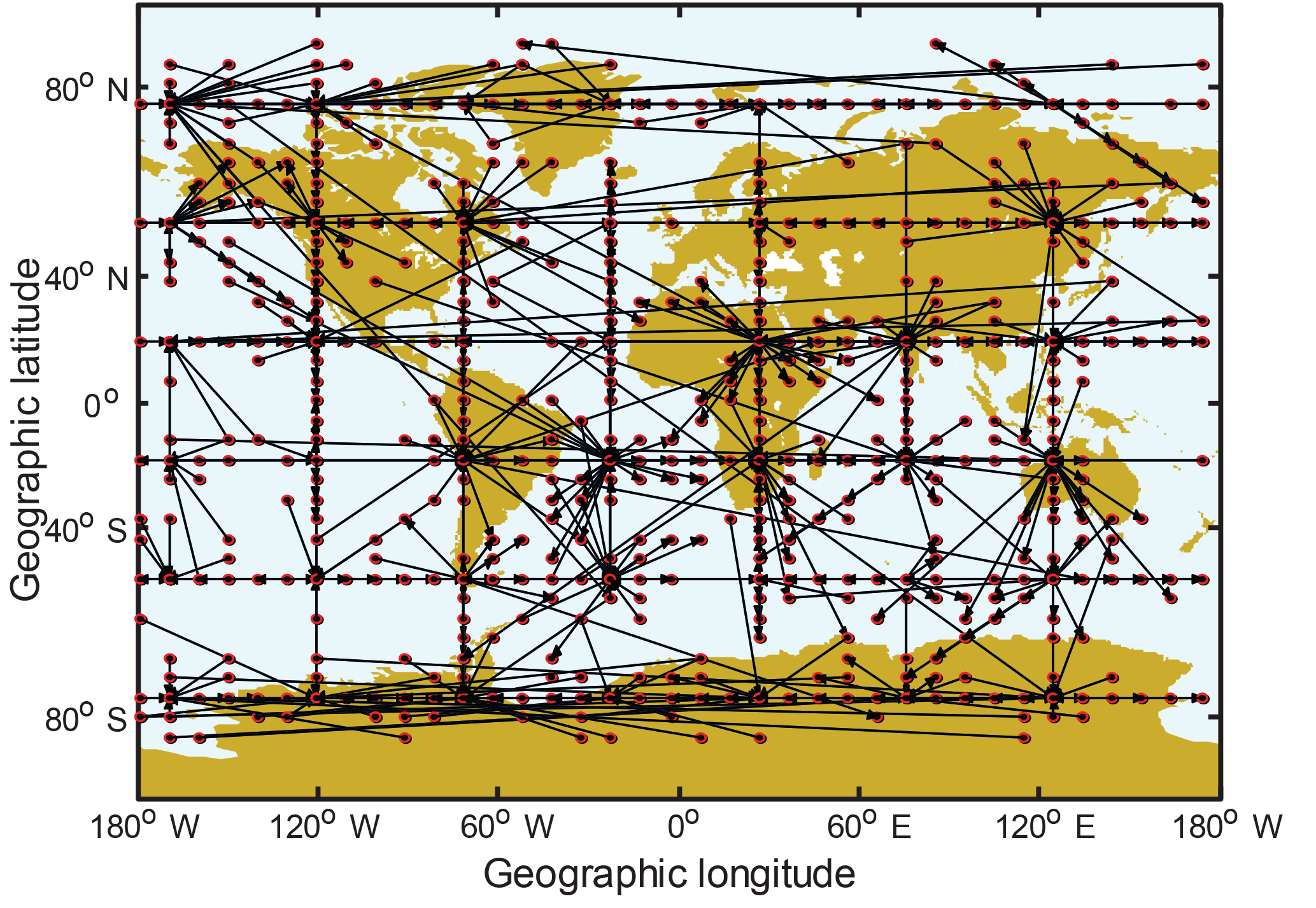
Figure 1The directed complex network of the ionosphere (in part). The network is developed from the GIM dataset by the FGS algorithm. The nodes indicate the GIM cells, while the directed edges represent causal interactions between cells.

Figure 2The degree distributions of the ionospheric network. Panel (a) shows the out-degree distribution; panel (b) shows the in-degree distribution. The red curves delineate the distribution fitting.
3.1 Degree distribution of the ionospheric network
To explore the influence of the VTEC's variation over a certain GIM cell, the degree of the ionospheric complex network is employed. As one of the most critical parameters to depict the nodes in a complex network, the degree is the number of edges the node possesses. Concerning ionospheric networks, the degree of a cell can be selected to quantify how many GIM cells display a causal interaction with that given cell in the globe; that is to say, cells with a large degree can influence large numbers of GIM cells. In the complex network, “hubs” refer to the nodes with large numbers of links that significantly exceed the average. Hubs have a significant effect on the system, which is described by the network. The emergence of hubs results from the scale-free property of networks (Barabási and Albert, 1999). Hence, to study the hub positions where the dynamic ionospheric processes mainly originate or converge, we have to check the scale-free topology of the degree distribution of the ionospheric network. The degree distribution is the probability distribution of these degrees over the whole network. For the directed ionospheric network, the degree distribution is divided into two different kinds, the out-degree distribution (the distribution of outgoing edges) and the in-degree distribution (the distribution of incoming edges). The degree distributions of the ionospheric network are shown in Fig. 2.
It has been reported that real complex networks often exhibit scale-free properties (Barabási and Albert, 1999). This means their degree distribution follows a power law, at least asymptotically; that is, the number of links of a given node exhibits a power-law distribution, , where k is the number of links. P(k) can be calculated by the statistical frequency, and γ is a parameter whose value is typically in the range . From the distributions shown in Fig. 2, it is hard to determine whether the observed degree is drawn from a power-law distribution or not. Clauset et al. (2009) presented a principled statistical framework for discerning power-law behavior in empirical data. As for the method shown in Clauset et al. (2009), we have tested the power-law hypothesis quantitatively. Both the results of the out-degree and in-degree distribution reject the hypothesis, indicating that the ionospheric network is not scale-free. Thus, most GIM cells have approximately the same number of edges, indicating that the causal interactions shown by the network of the global ionosphere are homogeneous. For the dynamic processes in the ionosphere, there is no unique spatial position acting as the source or sink. This property is completely different from that of the geomagnetic field. In other words, there are no visible hub GIM cells for the ionospheric variations. Moreover, from the curves of distribution fitting shown in Fig. 2, we can see that both the distributions are more likely Poisson, just like the network of climate (Tsonis et al., 2007).
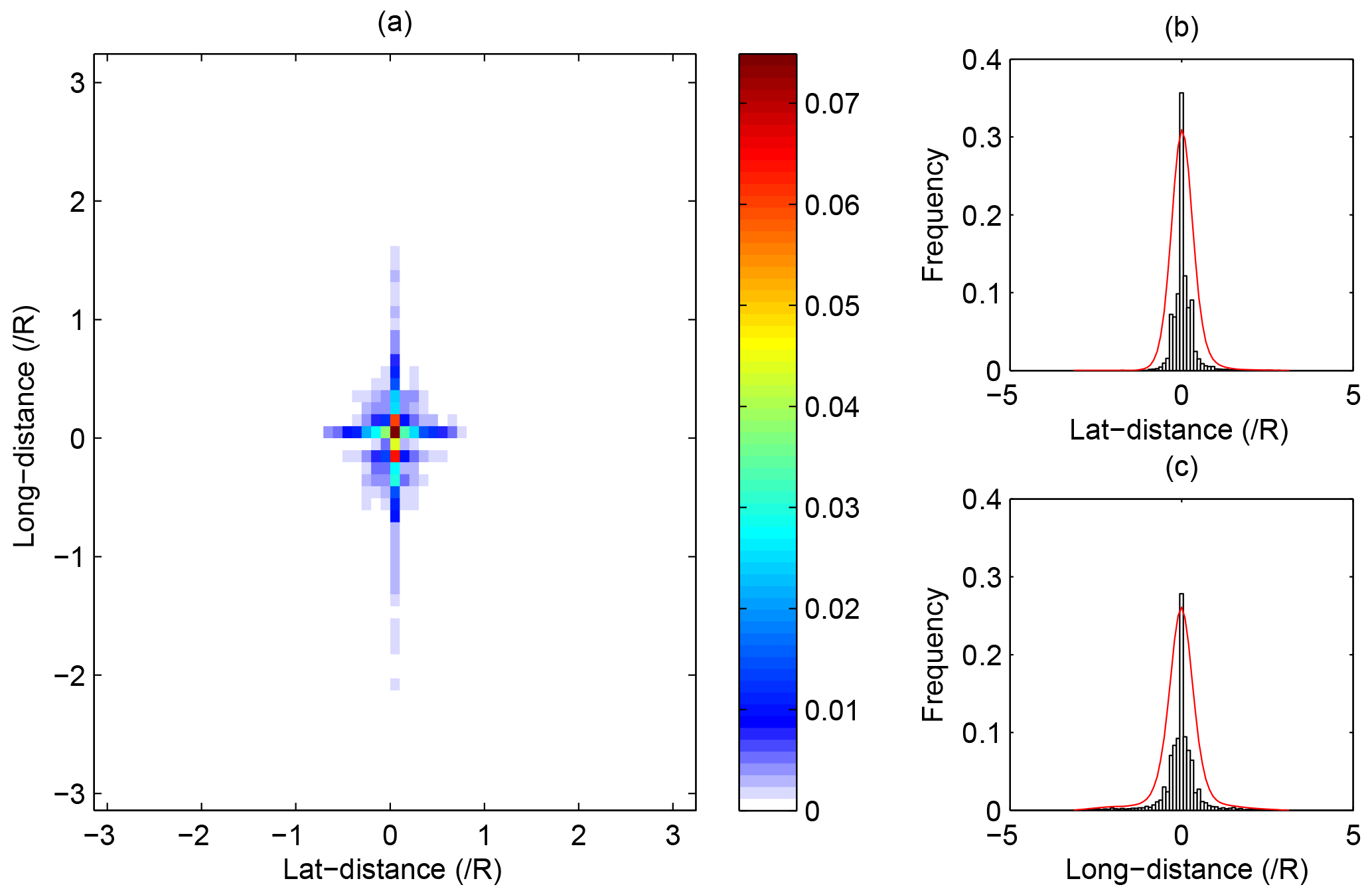
Figure 3The distribution of the directed edge distances in the global ionospheric network. Panel (a) shows the distribution of edges against the latitudinal and longitudinal distances; panel (b) shows the distribution of edges against their latitudinal distances; panel (c) shows the distribution of edges against their longitudinal distances. The red curves delineate the distribution fitting.
3.2 Distribution of the edge distances
The propagation of the dynamic processes is related to the transmission of energy or particles in the ionosphere. To analyze such a transport property, the distribution of the edge distances is calculated. The edge distance is defined by the geographical distance between the origin and destination of an edge. The height of the VTEC supplied by CODE is H = 450 km. As the measurements are on the earth which can be regarded as a sphere, the distances between any two positions can be calculated by the arc lengths on the sphere d=Rθ, where , R0 is the earth radius and θ is the corresponding central angle. Compared with the undirected probabilistic graphs, the directed ones can provide additional knowledge about the directions of the causal interactions within the ionosphere. To study the directional characteristics of the propagation of the dynamic ionospheric processes, the edge distances are mapped in the latitude and longitude directions.
The latitudinal distances are calculated by , where lat1 and lat2 are the latitudes of the origin and destination of the given edge. Meanwhile, the longitudinal distances are calculated by , where long1 and long2 are the longitudes of the origin and destination of the given edge. As the radii of different latitudinal circles are different, the radius of an equivalent latitudinal circle is calculated by the average of the radii of the two latitude circles on which the origin and destination of the given edge are located; i.e., . The positive signs of the distances represent the directions of edges and can either be eastward or northward. The result is shown in Fig. 3.
As is shown in Fig. 3a, the edges are mainly distributed around the origin of the coordinate system in the ionospheric network. Thus, the GIM cells are mostly connected with their spatial neighbors. The local connections indicate that, in the ionosphere, the propagation of the dynamic processes is primarily affected by the geospatial distance and almost satisfies the proximity principle in geospace. Furthermore, from the approximate symmetry along the x axis in Fig. 3b and c, we can discover that it is almost the same for the westward and eastward propagation of the dynamic processes, and also for the southward and northward. From Fig. 3b and c, we can see that the number of edges decreases as the absolute value of latitudinal and longitudinal distance increases. This phenomenon also reveals that the local interactions account for a considerable proportion in the ionospheric network. The proximal propagation may be due to the diffusion effects of charged particles in the ionosphere. In addition, comparing the standard deviations (SDs) of the edges' longitudinal and latitudinal distances, which are 0.53 and 0.28, we find that the distribution curve in the latitude direction is steeper than that in the longitude direction. Therefore, the rate of decrease along the latitude is larger than that along the longitude. Accordingly, the dynamic processes are propagated more efficiently along the longitude than along the latitude. Such a phenomenon may relate to the north–south currents or geomagnetic field in the ionosphere. Moreover, the ionospheric network is not entirely connected locally. Long-range edges emerge both along the latitude and longitude. The long-range propagation may be caused by the geomagnetic field or other global factors. Thus, the ionospheric network possesses a primarily ordered structure with some exceptional long-range connections.
3.3 Small-world structure of the ionospheric network
As for a complex network, the concept of being “stable” is defined as the high capability of the dynamics in the network to withstand disturbance attacks. In other words, the topology structure of the stable network cannot be easily destroyed and the dynamics can still be propagated throughout the network, even when some edges are removed by the disturbance attacks. “Efficient” is defined as the ability of rapid and easy propagation of dynamics in the network. In this subsection, we explore the small-world structure of the ionospheric network to examine the stability and efficiency of the ionosphere, which is regarded as a dynamical system.
Lying between the completely random and completely regular network, the small-world network is a type of graph in which any given node is likely to reach every other node by a small number of steps compared with the total number of network nodes (Gallos et al., 2007). The “six degrees of separation” in social networks is one of the most famous examples. Watts and Strogatz (1998) initially found that some networks can be highly clustered, like regular lattices, yet have small characteristic path lengths, like random graphs. Networks of such a nature are called small-world networks. To investigate the small-world structure of the ionospheric network, the original network has to be reduced to an undirected graph (Abe and Suzuki, 2006, 2009). Furthermore, to mathematically describe the small-world property, two critical parameters are often selected, which are the average clustering coefficient C and the average shortest path length L. Their definitions are shown in Eqs. (2)–(2).
Here, Ci is the local clustering coefficient of node i; ki is the degree of node i and Δi denotes the number of edges between the neighbors of node i, with node i itself being excluded. The global clustering coefficient C is defined as the average of all local clustering coefficients Ci. N is the number of nodes and dij denotes the length of the shortest path between the nodes i and j; dij is calculated by Dijkstra's algorithm (Newman, 2010). Thus, C describes the local connections in the ionospheric networks, while L characterizes a network's connectivity structure globally (Zerenner et al., 2014).
To quantitatively define a small-world network, values for the network properties must be compared with those values acquired from the equivalent random networks, which have the same degree as the given network on average. A measurement of “small-world-ness” is proposed as follows (Humphries and Gurney, 2008; Humphries et al., 2011):
Here, C and L are the average clustering coefficient and the average shortest path length of the given network, while Cr and Lr are those of the equivalent random network. If the given network fulfills the conditions σ>1 and , it meets the small-world criterion. To reduce the impact of randomness during the analysis of the ionospheric network, the results shown in Fig. 4 are calculated by 150 random networks.
From Fig. 4a and c, we can see that the results all satisfy σ>1 and . Shown in Fig. 4b and d, the frequencies are approximately Gaussian, and the SDs are 0.028 and 0.035. Such small SDs indicate that the results are close to the real values (the averages) 6.64 and 8.08. Therefore, the ionospheric network behaves as a small-world graph. The propagation of the dynamic processes in the ionosphere exhibits a small-world property. As was defined by Watts and Strogatz (1998), the small-world network possesses a small average shortest path length (compared to the regular network) and a large clustering coefficient (compared to the random network). When the number of edges per node is high, networks have a high clustering coefficient. In this case, accidental removal of some edges does not break the network into unconnected parts; the network is stable. On the other hand, a small average shortest path length L means faraway nodes can be connected as easily as nearby nodes. The smaller the L, the easier the propagation in the network. Within the networks with small L, the propagation of dynamics is efficient. Thus, small-world networks are stable and efficient in reacting to the abrupt variations (Tsonis et al., 2007).
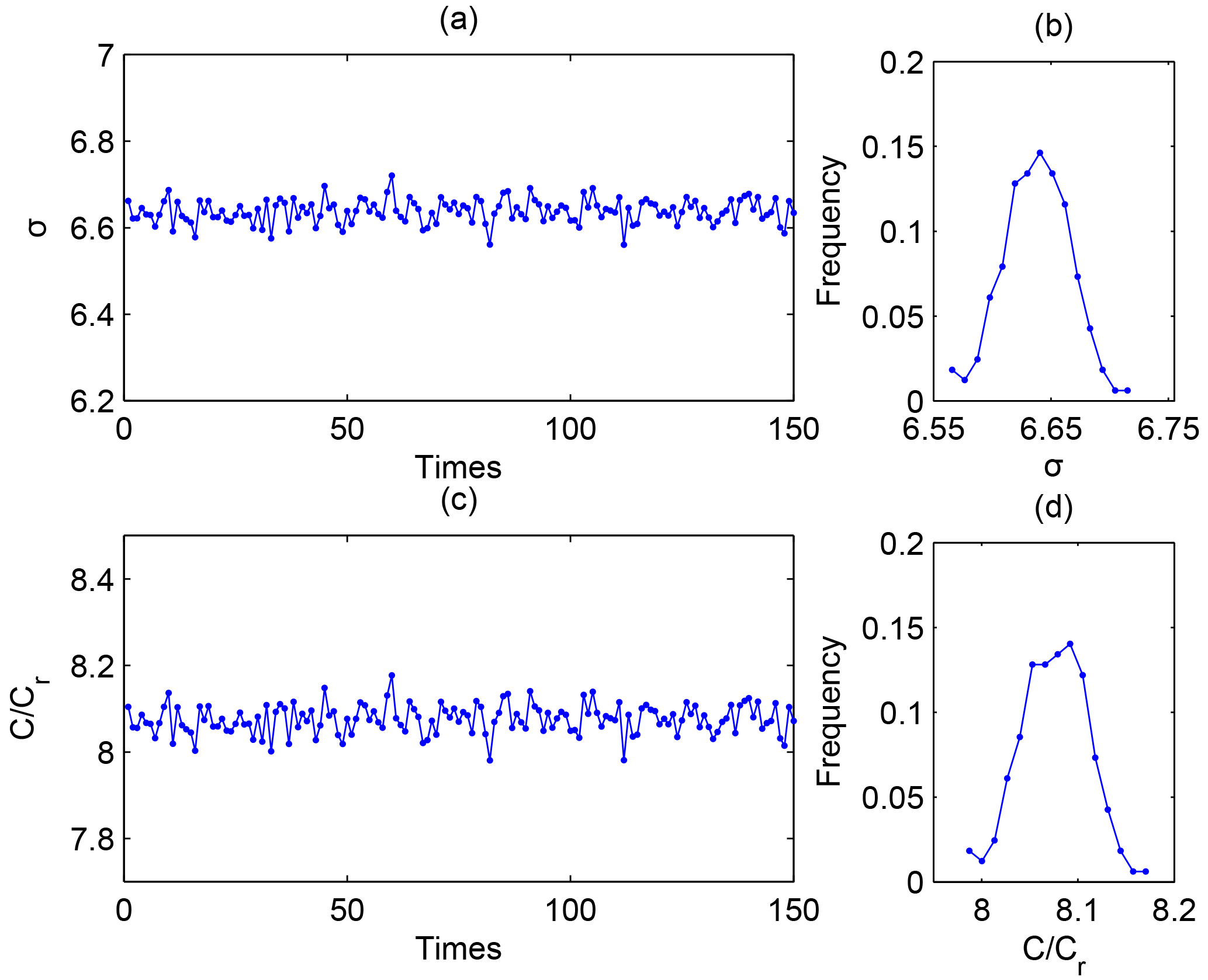
Figure 4The test of the small-world structure in the ionospheric network. Panel (a) shows the 150 results of σ; panel (b) shows the frequency of the results of σ; panel (c) shows the 150 results of C∕Cr; panel (d) shows the frequency of the results of C∕Cr.
As is shown by the results above, the ionospheric network is small-world with a small average shortest path length and a large clustering coefficient. Thus, the ionospheric network exhibits properties of stable networks and of networks where dynamic processes are transferred efficiently. For example, a solar flare may create a disturbance in the ionosphere at high latitudes. However, the small-world property of the ionospheric network allows the system to respond quickly and coherently to the anomalies introduced into the system. This dynamic propagation diffuses local anomalies, thereby reducing the possibility of prolonged local extremes and providing greater stability for the global ionosphere system. Thus, chances of major ionospheric shifts are reduced. The above theory and its application to the ionosphere data suggest that the ionosphere system may be inherently stable and efficient in transferring dynamics. Just as the small-world property in the atmosphere does (Donges et al., 2009b), such an ionospheric property also results from the teleconnections beyond the geospatial distance in the ionospheric network. Such teleconnections play an important role in stabilizing the ionosphere system and cause the dynamic ionospheric processes to be transferred efficiently (Donges et al., 2009b; Tsonis et al., 2007).
The ionosphere can be regarded as a spatially extended complex system. Therefore, the complex network is used to analyze the dynamic processes in the global ionosphere based on the VTEC from CODE. As a Bayesian probabilistic graph, the ionospheric network is constructed based on the conditional independence theory by the FGS algorithm. The edges of the network represent the causal relationships between any two GIM cells from a holistic perspective. We have analyzed the structure of the directed ionospheric network. The results of the power-law hypothesis test show that both the out-degree and in-degree distribution of the ionospheric network are not scale-free. The ionospheric network is homogenous. None of the geospatial positions play an eminently important role in the propagation of dynamic ionospheric processes. The importance of the ionosphere over various spatial locations in the propagation of the ionospheric dynamic processes is similar. Based on the latitudinal and longitudinal distances between the beginnings and ends of the edges, the joint distribution is analyzed to explore the propagation of the dynamic processes in the ionosphere. The results show that the edges principally exist between adjacent geographical locations, indicating that the propagation of the dynamic processes mainly satisfies the proximity principle in the ionosphere. Moreover, the joint distribution of the edge latitudinal and longitudinal distances shows that the dynamic processes travel more efficiently along the longitude than along the latitude. Also, the small-world structure is studied to examine the stability of the ionosphere. The small-world-ness of the ionospheric network is found to be larger than 1. Meanwhile, the clustering coefficient is larger than those of the equal random networks. Thus, the ionospheric network possesses a small-world property, which makes the ionosphere stable and efficient in the propagation of the dynamic processes. In general, the complex network provides a unique perspective in ionosphere research. Depending on the choice of nodes, edges and methods, ionospheric networks may take different forms to study different properties of the ionosphere.
Code is available by email request.
VTEC data are derived from CODE (ftp://ftp.aiub.unibe.ch/CODE/) (AIUB, 2018) in the form of a global ionospheric map.
The authors declare that they have no conflict of interest.
This work was supported by the National Natural Science Foundation of China
(41374154 and 41774156). We are grateful to Adam Woods from CIRES, University
of Colorado, David Skaggs Research Center, and Rolf Dach and Stefan Schaer
from the Astronomical Institute, University of Bern. They are all so kind to help us
with obtaining the data. Moreover, Shikun Lu would like to thank, in
particular, the ongoing and unwavering support from Taotao Sun over the
years.
Edited by: Stéphane
Vannitsem
Reviewed by: three anonymous referees
Abe, S. and Suzuki, N.: Complex-network description of seismicity, Nonlin. Processes Geophys., 13, 145–150, https://doi.org/10.5194/npg-13-145-2006, 2006. a, b
Abe, S. and Suzuki, N.: Main shocks and evolution of complex earthquake networks, Braz. J. Phys., 39, 428–430, 2009. a
AIUB: VTEC data, available at: ftp://ftp.aiub.unibe.ch/CODE/, last access: 22 March 2018.
Baiesi, M. and Paczuski, M.: Complex networks of earthquakes and aftershocks, Nonlin. Processes Geophys., 12, 1–11, https://doi.org/10.5194/npg-12-1-2005, 2005. a
Barabási, A. L. and Albert, R.: Emergence of Scaling in Random Networks, Science, 286, 509–512, 1999. a, b
Clauset, A., Shalizi, C. R., and Newman, M. E. J.: Power-Law Distributions in Empirical Data, Siam Rev., 51, 661–703, 2009. a, b
Donges, J. F., Zou, Y., Marwan, N., and Kurths, J.: The backbone of the climate network, Europhys. Lett., 87, 48007–48012, 2009a. a
Donges, J. F., Zou, Y., Marwan, N., and Kurths, J.: Complex networks in climate dynamics – Comparing linear and nonlinear network construction methods, The European Physical Journal Special Topics, 174, 157–179, 2009b. a, b, c
Ebert-Uphoff, I. and Deng, Y.: A new type of climate network based on probabilistic graphical models: Results of boreal winter versus summer, Geophys. Res. Lett., 39, L19701-1–L19701-7, 2012. a
Ercha, A., Huang, W., Yu, S., Liu, S., Shi, L., Gong, J., Chen, Y., and Hua, S.: A regional ionospheric TEC mapping technique over China and adjacent areas on the basis of data assimilation, J. Geophys. Res.-Space, 120, 1–13, 2015. a
Gallos, L. K., Song, C., and Makse, H. A.: A review of fractality and self-similarity in complex networks, Physica A, 386, 686–691, 2007. a
Guo, J., Li, W., Liu, X., and Kong, Q.: Temporal-Spatial Variation of Global GPS-Derived Total Electron Content 1999–2013, Plos One, 10, 1–21, https://doi.org/10.1371/journal.pone.0133378, 2015. a
Hlinka, J., Hartman, D., Vejmelka, M., Runge, J., Marwan, N., Kurths, J., and Palus, M.: Reliability of Inference of Directed Climate Networks Using Conditional Mutual Information, Entropy, 15, 2023–2045, 2013. a
Humphries, M. D. and Gurney, K.: Network 'small-world-ness': a quantitative method for determining canonical network equivalence, Plos One, 3, e0002051-1–e0002051-10, 2008. a
Humphries, M. D., Gurney, K., and Prescott, T. J.: The brainstem reticular formation is a small-world, not scale-free, network, P. Roy. Soc. B-Biol. Sci., 273, 503–511, 2011. a
Jiménez, A., Tiampo, K. F., and Posadas, A. M.: Small world in a seismic network: the California case, Nonlin. Processes Geophys., 15, 389–395, https://doi.org/10.5194/npg-15-389-2008, 2008. a
Kelly, M.: The Earth's Ionosphere: Plasma Physics and Electrodynamics, 2nd edn., Academic Press (Elsevier), San Diego, CA, USA, 2009. a
Koller, D. and Friedman, N.: Probabilistic Graphical Models: Principles and Techniques – Adaptive Computation and Machine Learning, MIT Press, Cambridge, MA, USA, 2009. a, b, c
Murphy, K. P.: Machine Learning: A Probabilistic Perspective, MIT Press, Cambridge, MA, USA, 2012. a
Newman, M.: Networks: An Introduction, Oxford University Press Inc., Oxford, UK, 2010. a
Nocke, T., Buschmann, S., Donges, J. F., Marwan, N., Schulz, H.-J., and Tominski, C.: Review: visual analytics of climate networks, Nonlin. Processes Geophys., 22, 545–570, https://doi.org/10.5194/npg-22-545-2015, 2015. a
Peron, T. K. D., Comin, C. H., Amancio, D. R., da F. Costa, L., Rodrigues, F. A., and Kurths, J.: Correlations between climate network and relief data, Nonlin. Processes Geophys., 21, 1127–1132, https://doi.org/10.5194/npg-21-1127-2014, 2014. a
Podolská, K., Truhlík, V., and Tísková, L.: Analysis of ionospheric parameters using graphical models, in: EGU General Assembly Conference, 2–7 May 2010, Vienna, Austria, 2010. a
Podolská, K., Truhlík, V., and Tísková, L.: Study of Correlationships between Main Ionospheric Parameters by Stochastic Modeling, in: EGU General Assembly Conference, 22–27 April 2012, Vienna, Austria, 2012. a
Ramsey, J., Glymour, M., Sanchezromero, R., and Glymour, C.: A million variables and more: the Fast Greedy Equivalence Search algorithm for learning high-dimensional graphical causal models, with an application to functional magnetic resonance images, International Journal of Data Science and Analytics, 3, 121–129, 2017. a
Schwarz, G.: Estimating the Dimension of a Model, Ann. Stat., 6, 15–18, 1978. a
Suteanu, M.: Scale free properties in a network-based integrated approach to earthquake pattern analysis, Nonlin. Processes Geophys., 21, 427–438, https://doi.org/10.5194/npg-21-427-2014, 2014. a
Tsonis, A. A., Swanson, K. L., and Wang, G.: On the Role of Atmospheric Teleconnections in Climate, J. Climate, 21, 2990–3001, 2007. a, b, c
Wang, J., Jiang, C., Quek, T. Q., and Ren, Y.: The Value Strength Aided Information Diffusion in Online Social Networks, in: IEEE Global Conference on Signal and Information Processing (GlobalSIP), 1–6, Washington, DC, USA, 2016a. a
Wang, J., Jiang, C., Quek, T. Q., Wang, X., and Ren, Y.: The Value Strength Aided Information Diffusion in Socially-Aware Mobile Networks, IEEE Access, 4, 3907–3919, 2016b. a
Watts, D. J. and Strogatz, S. H.: Collective dynamics of 'small-world' networks, Nature, 393, 440–442, 1998. a, b
Wei, N., SHI, and Zou, R.: Analysis and Assessments of IGS Products Consistencies, Geomatics and Information Science of Wuhan University, 34, 1363–1367, 2009. a
Zerenner, T., Friederichs, P., Lehnertz, K., and Hense, A.: A Gaussian graphical model approach to climate networks, Chaos an Interdisciplinary Journal of Nonlinear Science, 24, 023103-1–023103-10, 2014. a, b, c