Evolution of fractality in space plasmas of interest to geomagnetic activity

We studied the temporal evolution of fractality for geomagnetic activity, by calculating fractal dimensions from the Dst data and from a magnetohydrodynamic shell model for turbulent magnetized plasma, which may be a useful model to study geomagnetic activity under solar wind forcing. We show that the shell model is able to reproduce the relationship between the fractal dimension and the occurrence of dissipative events, but only in a certain region of viscosity and resistivity values. We also present preliminary results of the application of these ideas to the study of the magnetic field time series in the solar wind during magnetic clouds, which suggest that it is possible, by means of the fractal dimension, to characterize the complexity of the magnetic cloud structure.

1 Introduction

There is a nontrivial magnetic interaction between Sun and Earth, coupled by the solar wind, leading to a rich variety of phenomena, which has attracted interest to the study of space plasmas for decades, and more recently to the possibility of forecasting space weather, an issue of large relevance in our increasingly technology-dependent society.

Various models and techniques have been developed to study the plasma behavior in the Sun–Earth system. Of these, the study of complexity has been of great interest, as it is capable of providing new insights regarding universal behavior related to geomagnetic activity, turbulence in laboratory plasmas or the solar wind, to name a few (Dendy et al., 2007; Klimas et al., 2000; Takalo et al., 1999; Chang and Wu, 2008; Valdivia et al., 1988). In particular, it has been suggested that various magnetized plasma systems are in a self-organized critical state, exhibiting fractal and multifractal features which relate them to a broader class of complex systems. This has been the case in studies on the Earth's magnetosphere (Chang, 1999; Valdivia et al., 2005, 2003, 2006, 2013), the solar wind (Macek, 2010), the solar photosphere, and solar corona (Berger and Asgari-Targhi, 2009; Dimitropoulou et al., 2009). Some authors have discussed the relationship between the fractal dimension and physical processes in magnetized plasmas in the Sun–Earth system, including the possibility of forecasting geomagnetic activity (Aschwanden and Aschwanden, 2008; Uritsky et al., 2006; Georgoulis, 2012; McAteer et al., 2005, 2010; Dimitropoulou et al., 2009; Conlon et al., 2008; Chapman et al., 2008; Kiyani et al., 2007).

In our work we use the box-counting fractal dimension (Addison, 1997), which is a simple measure of complexity, and which has an intuitive meaning. Certainly, a single fractal dimension cannot provide all information on complexity for systems in general. Moreover, most systems of interest also have multifractal features, such as the magnetospheric system (Chang, 1999), models of turbulence (Kadanoff et al., 1995; Pisarenko et al., 1993), and the solar wind (Chapman et al., 2008); but it is interesting to note that it does describe some relevant features of these time series' complexity, as it has been successfully used in previous works relevant to the Sun–Earth system (Osella et al., 1997; Kozelov, 2003; Gallagher et al., 1998; Georgoulis, 2012; Lawrence et al., 1993; Cadavid et al., 1994; McAteer et al., 2005). We will thus use the box-counting as a fast approach and a first step to detect universal features worth further study. In addition, we will calculate fractal dimensions based on a scatter diagram (see e.g., Witte and Witte, 2009), unlike some previous studies, where different methods or data (Kozelov, 2003; Uritsky et al., 2006; Balasis et al., 2006; Dias and Papa, 2010) were used.

These ideas were implemented by us in Domínguez et al. (2014) to study the Dst time series and solar magnetograms and the possible correlation between solar and geomagnetic activities as evidenced by the box-counting fractal dimension. Individual events, complete years of high geomagnetic activity, and the full 23rd solar cycle were studied with this technique, successfully finding that the fractal dimension, and more specifically its evolution, has – despite its simplicity – relevant information on the complex behavior of these systems and their eventual correlation.

The results mentioned above were robust, in the sense that they were observed across a wide range of timescales, which suggests that any model describing the dynamics of geomagnetic activity should reproduce a similar fractal behavior. This is our motivation to study a shell model for magnetohydrodynamic (MHD) turbulence within this framework.

Evidence of turbulence in the Earth's magnetosphere has been found by various spacecraft observations (Nykyri et al., 2006; Sundkvist et al., 2005; Zimbardo et al., 2008), and several authors have studied magnetospheric MHD turbulence (see, e.g., Borovsky, 2004; Hwang et al., 2011; El-Alaoui et al., 2012). However, given the large number of degrees of freedom, simulation of turbulent systems has a large computational cost, which has led to the development of analytical models, which, while sharing statistical properties of the systems under study, depend only on a few degrees of freedom (Chapman et al., 1998; Valdivia et al., 2006).

At an intermediate level between these models and first-principles approaches we find shell models, consisting of a set of coupled equations which are similar to the spectral Navier–Stokes equation, but which are also low dimensional models. They have been successfully used to describe turbulence in magnetized fluids, being able to deal with large Reynolds numbers without the associated computational cost of simulations based on first principles and nonlinear fluid equations (Ditlevsen, 2011), and describing the main statistical properties of MHD turbulence (Chapman et al., 2008).

In fact, it has been shown that dissipative events in shell models can be taken to represent solar flares and that their distribution follows the same power-law statistics as observed in turbulent magnetized plasmas (Boffetta et al., 1999; Lepreti et al., 2004; Carbone et al., 2002). As suggested in Lepreti et al. (2004), flares and geomagnetic activity could be the results of dissipation bursts within a turbulent environment.

In a previous work (Domínguez et al., 2017), we have applied the box-counting fractal dimension to study the complexity in an MHD shell model, analyzing the correlation between it and the energy dissipation rate, showing that, for certain values of the viscosity and the magnetic diffusivity, the fractal dimension exhibits correlation with the occurrence of bursts, similar to what had been found with geomagnetic data (Domínguez et al., 2014). This suggests that shell models do not only reproduce the power-law statistics of dissipative events in turbulent plasmas but also some features of its fractal behavior.

In this paper we review our results in this field, where complexity in magnetic field time series is measured by means of the fractal dimension. Thus, we characterize events such as geomagnetic storms by means of analyzing the Dst time series on various timescales (described in Sects. 2–3, and discussed previously in more detail in Domínguez et al., 2014) and the occurrence of dissipative events in an MHD shell model simulation (Sect. 4; see Domínguez et al., 2017 for more details). We also present preliminary results dealing with spacecraft data for the solar wind, related to the appearance of magnetic clouds (Sect. 5).

2 Fractal dimension

We are interested in estimating the fractal dimension to various time series for magnetic data. We now explain the method, using the hourly Dst time series as an example (World Data Center for Geomagnetism, http://wdc.kugi.kyoto-u.ac.jp/caplot/index.html).

Fractal dimensions can be defined in various ways in general, and for a specific time series in particular ways as well (Addison, 1997; Theiler, 1990). In general it can be said that they are numbers, which can be noninteger, measuring the complexity of a data set. In this work, we estimate the fractal dimension using the box-counting method (Addison, 1997) as shown below. First, a scatter diagram is obtained from each Dst time series, by plotting each datum versus the next one (see Fig. 1).

Then, the scatter diagram is divided into square cells of a certain size ϵ. By decreasing ϵ, we eventually find a region where the number of cells containing points scales as a power law with ϵ:

$$\begin{array}{}\text{(1)}& N\left(\mathit{ϵ}\right)\propto {\mathit{ϵ}}^{-D},\end{array}$$

where D is the scatter plot box-counting dimension. We estimate the error in D through the least-squares fit for the slope.

Further details and discussion on the method can be found in Domínguez et al. (2014).

The method as stated above was applied to the Dst time series where, given the width of the data windows used (the criterion is discussed in Sect. 3) and the time resolution of the data (one point per hour), it only made sense to build the scatter plot with consecutive data points.

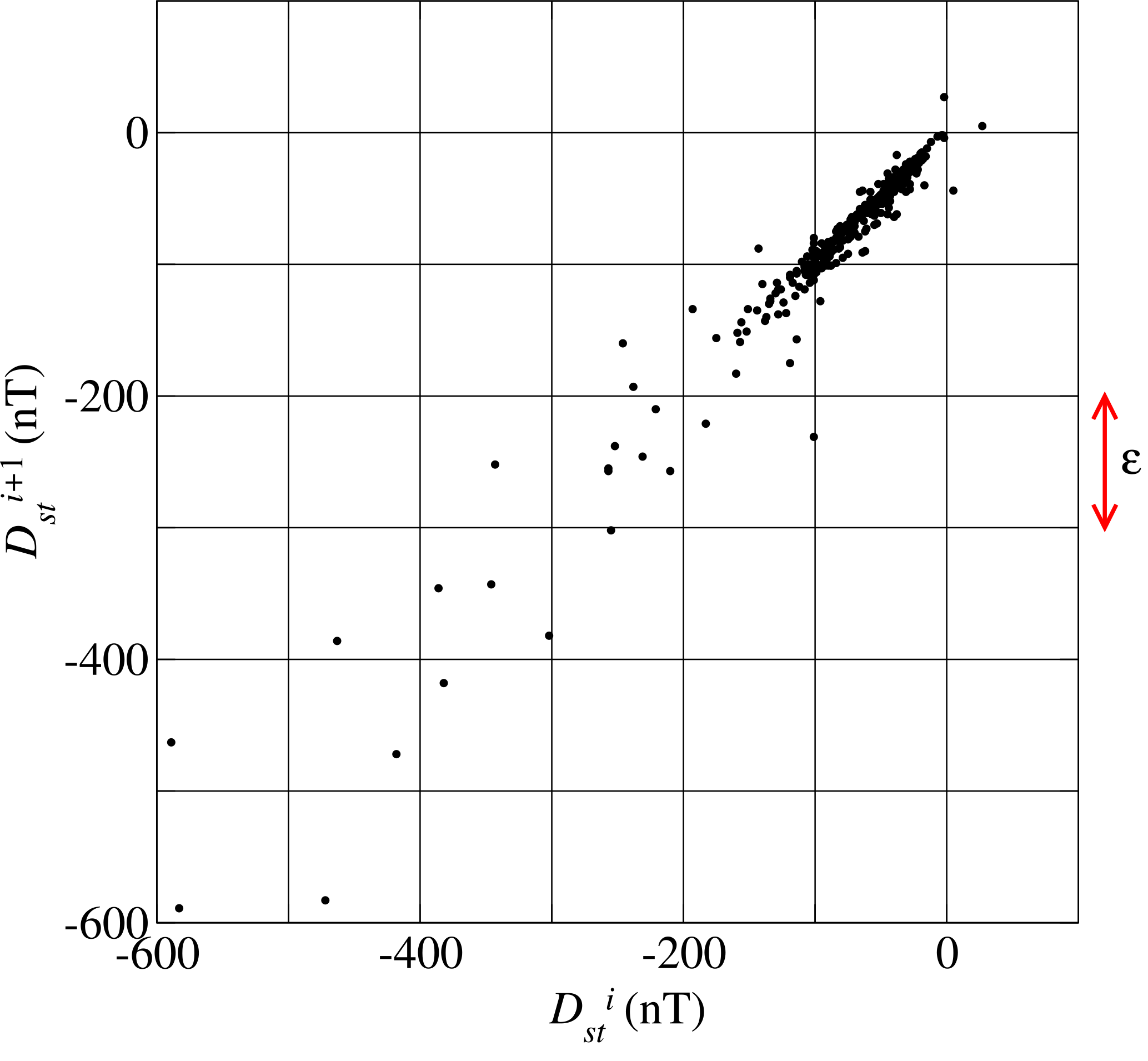
Figure 1 Scatter diagram for Dst time series, using data from 6 to 20 March 1989, containing a large geomagnetic storm. (Taken from Domínguez et al., 2014.)

However, when resolution is larger, as is the case with simulation and solar wind data, it is possible to consider different time delays. Thus, the scatter plot can be built by plotting the ith data in the set, versus the (i+j)th data, with j≥1 in general, and then the fractal dimension calculated depends on j, D_j. This was the approach in Domínguez et al. (2017), and it is presented here in Sects. 4 and 5.

3 Dst time series

Some studies (Balasis et al., 2009; Papa and Sosman, 2008) have suggested that there is a relationship between the intensity and the complexity of the Dst time series. Here, we will first apply the technique discussed in Sect. 2 to investigate whether there is a connection between the level of geomagnetic activity and the fractal dimension of the Dst index.

Following Domínguez et al. (2014), we are interested in testing the usefulness of the method by first studying strong, clear events. Thus, we identify “storm states” and “quiet states” by locating Dst peaks, such that Dst < −220 nT, which corresponds to intense magnetic storms. A storm state is defined by a 2-week window centered on the minimum Dst value. This is done considering the typical timescale of a geomagnetic storm (Tsurutani and Gonzalez, 1994; Gonzalez et al., 1994). Quiet states simply correspond to the time window between consecutive storm states. This is illustrated in Fig. 2, corresponding to the year 1989, where four peaks are found.

In the following, states within a year are labeled by integer numbers starting from 1. A fractal dimension is then calculated for each storm and each quiet state in the same year. Results for 1989 are shown in Fig. 3.

Similar plots for 5 years of high geomagnetic activity were obtained (Domínguez et al., 2014). In general, storm states are found to have a smaller fractal dimension than quiet states immediately before and after them, although there does not seem to be a clear correlation with the value of Dst itself (Domínguez et al., 2014). Thus, our statement on the decrease of the fractal dimension is an argument about its variation, rather than about its actual value. These results are consistent with Balasis et al. (2009), where it is shown that the Tsallis entropy of the Dst time series decreases during intense magnetic storms (Dst < −150 nT in their case).

We have also studied variable width windows around a storm and moving windows across storms, and results have been consistent with the findings discussed.

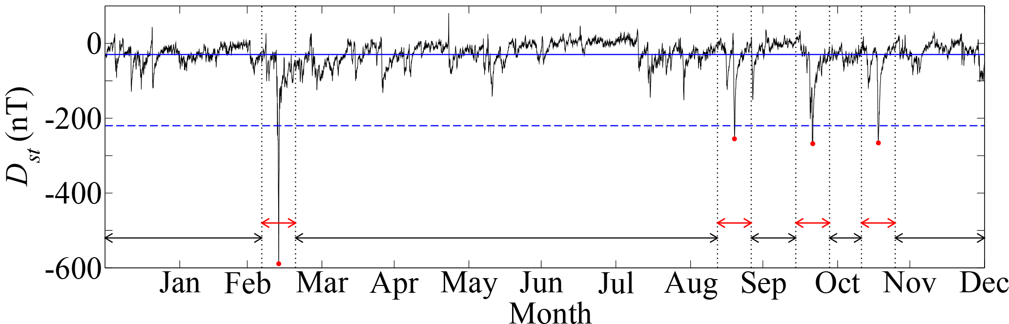
Figure 2 Storm and quiet states in the Dst time series for 1989, also indicating the average value of the Dst index (horizontal line), and the threshold used to identify storms (dashed line). Red (black) arrows indicate storm (quiet) states. (Taken from Domínguez et al., 2014.)

In effect, as a window is widened around a storm, more “quiet” data are considered, and thus the fractal dimension of the data inside the window should increase. This is actually the case, as shown for instance in Fig. 4, where results for four storms are taken, selected because they are isolated enough to allow enlargement of the window around them without overlapping with neighboring storms (Domínguez et al., 2014).

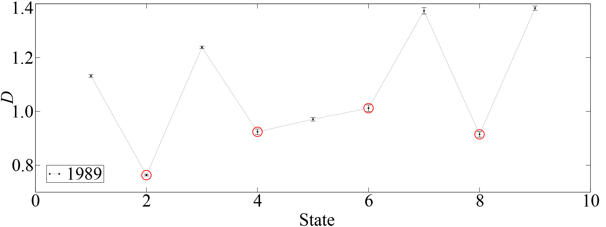
Figure 3 Box-counting dimension D for storm and quiet states for the year 1989. Labels in the horizontal axis represent consecutive states as mentioned in Sect. 3. Storm states are marked with red circles, whereas errors are taken from the least-squares linear fit. (Taken from Domínguez et al., 2014.)

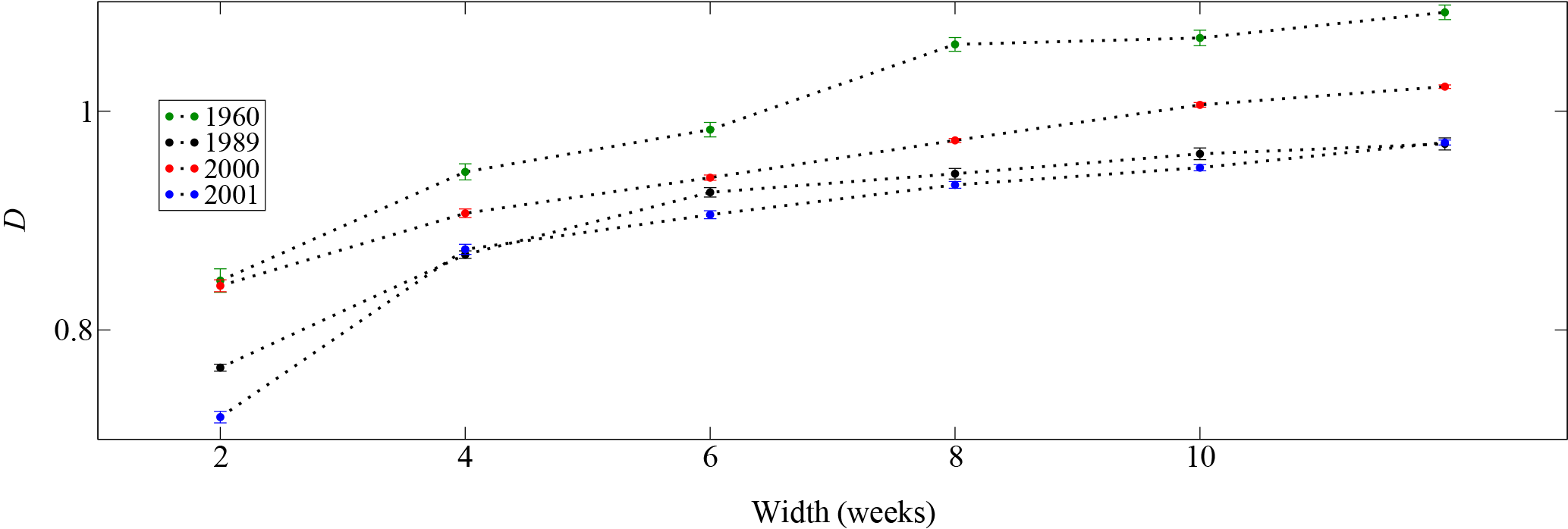
Figure 4 Box-counting dimension D for a storm state, as a function of window width. Lines correspond to storms on 1 April 1960, 13 March 1989, 6 April 2000, and 30 March 2001. (Taken from Domínguez et al., 2014.)

Regarding the moving windows analysis, results are illustrated for the 13 March 1989 storm in Fig. 5, comparing it with the Dst index.

As shown in Domínguez et al. (2014), the box-counting dimension of the Dst index decreases as the storm approaches for all cases studied. Moreover, this decrease occurs before the window includes the geomagnetic storm, as marked by the vertical lines in Fig. 5. Whether this is relevant for forecasting geomagnetic storms needs further study, as it may simply be due to an increase of the intermittency in the time series, unrelated to the upcoming dissipative event.

In Domínguez et al. (2014), systematic calculations of cross correlation between Dst and D were performed using year-long data for 1960, 1989, 2000, 2001, and 2003, suggesting that the decrease of the box-counting dimension is a robust feature.

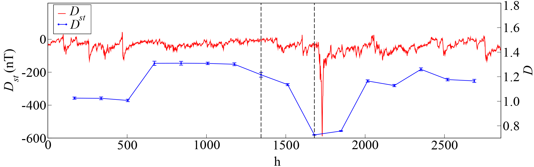
Figure 5 Box-counting dimension D (blue) and Dst index (red) for the 13 March 1989 geomagnetic storm. D decreases before the storm in the windows within the vertical lines. (Taken from Domínguez et al., 2014.)

4 MHD shell model

Given the intrinsic difficulties in using direct numerical simulations to describe turbulent flows, especially for large Reynolds numbers, shell models have been used for years in order to reproduce the nonlinear dynamics of fluid systems in large dynamical ranges, but with fewer degrees of freedom (Obukhov, 1971; Gledzer, 1973; Yamada and Ohkitani, 1988). An MHD shell model (Boffetta et al., 1999), in particular, is a dynamical system which aims to reproduce the main features of MHD turbulence. The model corresponds to a simplified version of the Navier–Stokes or MHD equations for turbulence, which conserves some of its invariants in the limit of no dissipation.

In this work, we use the MHD shell model proposed by Gledzer, Okhitani, and Yamada (GOY shell model), which describes the dynamics of the energy cascade in MHD turbulence (Lepreti et al., 2004). The model is built up by dividing the wave-vector space (k-space) in N discrete shells of radius k_n=k₀2ⁿ ($n=\mathrm{0},\mathrm{1},\mathrm{\dots },N$). Then, two complex dynamical variables u_n(t) and b_n(t), representing velocity and magnetic field increments on an eddy scale $l\sim k_n^{-\mathrm{1}}$, are assigned to each shell.

The model consists of the following set of ordinary differential equations:

$$\begin{array}{ll}{\displaystyle \frac{\mathrm{d}{u}_n}{\mathrm{d}t}}=& {\displaystyle }-\mathit{\nu }{k}_n^{\mathrm{2}}{u}_n+i{k}_n\left(u_{n+\mathrm{1}}{u}_{n+\mathrm{2}}-b_{n+\mathrm{1}}{b}_{n+\mathrm{2}}\right)\\ {\displaystyle }& {\displaystyle }-i{k}_n\left\{{\displaystyle \frac{\mathrm{1}}{\mathrm{4}}}\left(u_{n-\mathrm{1}}{u}_{n+\mathrm{1}}-b_{n-\mathrm{1}}{b}_{n+\mathrm{1}}\right)\right.\\ \text{(2)}& {\displaystyle }& {\displaystyle }{\left.+{\displaystyle \frac{\mathrm{1}}{\mathrm{8}}}\left(u_{n-\mathrm{2}}{b}_{n-\mathrm{1}}-b_{n-\mathrm{2}}{u}_{n-\mathrm{1}}\right)\right\}}^{\ast }+f_n,{\displaystyle \frac{\mathrm{d}{b}_n}{\mathrm{d}t}}=& {\displaystyle }-\mathit{\eta }{k}_n^{\mathrm{2}}{b}_n+i{k}_n{\displaystyle \frac{\mathrm{1}}{\mathrm{6}}}\left(u_{n+\mathrm{1}}{b}_{n+\mathrm{2}}-b_{n+\mathrm{1}}{u}_{n+\mathrm{2}}\right)\\ {\displaystyle }& {\displaystyle }-i{k}_n{\displaystyle \frac{\mathrm{1}}{\mathrm{6}}}\left\{\left(u_{n-\mathrm{1}}{b}_{n+\mathrm{1}}-b_{n-\mathrm{1}}{u}_{n+\mathrm{1}}\right)\right.\\ \text{(3)}& {\displaystyle }& {\displaystyle }{\left.+\left(u_{n-\mathrm{2}}{b}_{n-\mathrm{1}}-b_{n-\mathrm{2}}{u}_{n-\mathrm{1}}\right)\right\}}^{\ast }+g_n,\end{array}$$

where ν and η are, respectively, the kinematic viscosity and the resistivity; f_n and g_n are external forcing terms acting, respectively, on the velocity and magnetic fluctuations. The symbol ^* represents a complex conjugate quantity. The nonlinear terms have been obtained by imposing quadratic nonlinear coupling between neighboring shells and the conservation of three MHD ideal invariants (Gloaguen et al., 1985; Lepreti et al., 2004).

The forcing terms are calculated according to the Langevin equation

$$\begin{array}{}\text{(4)}& {\displaystyle \frac{\mathrm{d}{\stackrel{\mathrm{̃}}{f}}_n}{\mathrm{d}t}}=-{\displaystyle \frac{{\stackrel{\mathrm{̃}}{f}}_n}{{\mathit{\tau }}_{\mathrm{0}}}}+\stackrel{\mathrm{̃}}{\mathit{\mu }},\end{array}$$

where ${\stackrel{\mathrm{̃}}{f}}_n=f_n$ or g_n, τ₀ is a characteristic time of the largest shell, and $\stackrel{\mathrm{̃}}{\mathit{\mu }}$ is a Gaussian white noise of width σ.

The magnetic energy dissipation rate is defined as

$$\begin{array}{}\text{(5)}& {\mathit{ϵ}}_b\left(t\right)=\mathit{\eta }\sum _{n=\mathrm{1}}^N{k}_n^{\mathrm{2}}\left|b_n^{\mathrm{2}}\right|.\end{array}$$

In our simulation, we set σ=0.01, τ₀=0.25, take N=19 shells, and force the system on the largest shell ($f_{\mathrm{1}},g_{\mathrm{1}}\ne \mathrm{0}$). Similar parameters have been considered in previous studies using this model for the modeling of solar flares' statistics (Boffetta et al., 1999; Lepreti et al., 2004; Nigro et al., 2004).

We numerically integrate the shell model Eqs. (2)–(2) for various values of ν and η, and then we calculate the magnetic energy dissipation rate ϵ_b(t) (Eq. 3).

Figure 6 shows a typical time behavior for ϵ_b(t).

Previous works have compared the statistics of bursts in turbulent systems with the statistics of dissipative events in the shell model (Boffetta et al., 1999; Lepreti et al., 2004; Carbone et al., 2002). There, peaks in the ϵ_b(t) time series have been associated with dissipative events in the magnetized plasma. Following the ideas in Sect. 3 regarding the size of events considered, we focus only on the largest peaks in the ϵ_b(t) time series, specifically, on dissipative events where the maximum value is larger than $\langle {\mathit{ϵ}}_b\rangle +n\stackrel{\mathrm{̃}}{\mathit{\sigma }}$ where 〈ϵ_b〉 is the average value of ϵ_b over all simulation time, $\stackrel{\mathrm{̃}}{\mathit{\sigma }}$ is the standard deviation of the ϵ_b time series in that window, and n is a certain integer. In this paper we discuss only results for n=10, but in Domínguez et al. (2017) n=5 was also considered, in order to assess the robustness of the results. Our aim is to study the dependence of the conclusions on ν and η in Eqs. (2) and (2).

We now apply the same techniques used to study the Dst index, as described in Sects. 2–3, to the ϵ_b(t) time series.

We first notice that, in general, setting parameters ν and η with arbitrary values yields ϵ_b(t) series, which do not have the necessary intermittency level to resemble the Dst time series. Compare, for instance, the different panels in Fig. 16 in Domínguez et al. (2017), which show that Pm=0.2 leads to a very noisy output, unlike simulations with Pm=1.0 or 2.0, where individual, large peaks can be easily identified from the background. In fact, previous studies have shown that the statistics of bursts follows a power law for Pm=1 (Boffetta et al., 1999; Lepreti et al., 2004; Carbone et al., 2002), and for this reason we start by taking $\text{Pm}=\mathit{\nu }/\mathit{\eta }=\mathrm{1}$.

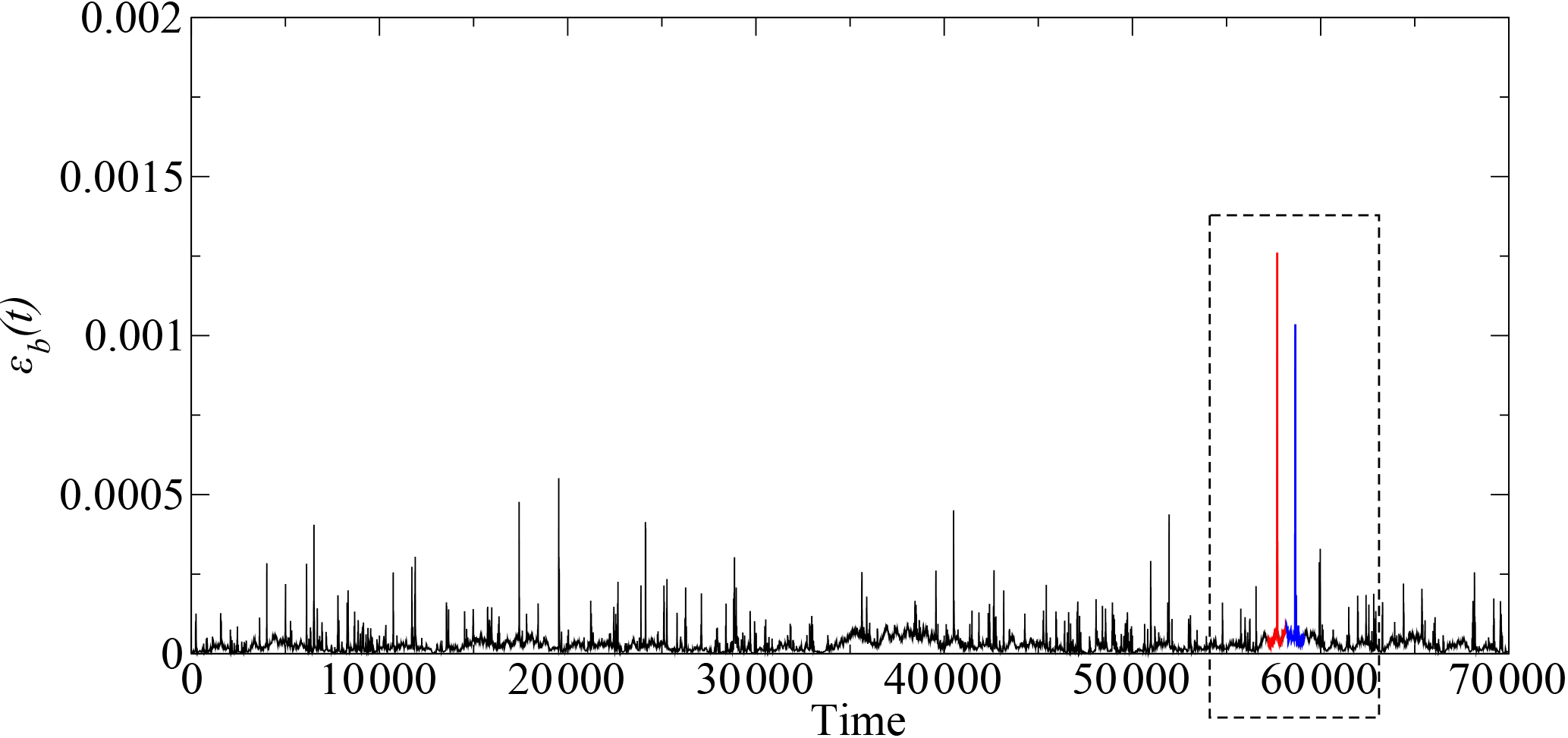
Figure 6 Time series of ϵ_b(t), Eq. (3), with $\mathit{\nu }=\mathit{\eta }={\mathrm{10}}^{-\mathrm{4}}$ in the shell model. The red and blue regions inside the dashed box correspond to an active state, as explained later in the text. (Taken from Domínguez et al., 2017.)

Now, we need to define “active states” and quiet states. For the Dst case (Domínguez et al., 2014) there are natural timescales which were used to define the occurrence and the duration of a geomagnetic storm. However this is not available for the output of the shell model, and our approach was to inspect the data to gain intuition on this. As described in detail in Domínguez et al. (2017), we take $\text{Pm}=\mathit{\nu }/\mathit{\eta }=\mathrm{1}$ as fixed, and then a wide range of values of ν, in the interval ${\mathrm{10}}^{-\mathrm{12}}\le \mathit{\nu }\le {\mathrm{10}}^{-\mathrm{1}}$. For each parameter set, we solve the shell model equations using a time step of $\mathrm{d}t={\mathrm{10}}^{-\mathrm{4}}$ and for 7×10⁸ iterations. We conclude that n=10 is enough to filter most events, except for the largest ones.

Regarding the width of an active state, Fig. 6 is, among the various simulations we performed, the only case where two clear dissipative events were both close and distinguishable from each other. Thus we take this as a reference run, and since the separation between both peaks is 96 000 time steps, we define an active state in the shell model output as a window of 96 000 time steps, centered around a peak in the magnetic energy dissipation. Therefore, Fig. 6 shows two adjacent active states.

We now analyze the output of the simulation for given values of ν and n, identify active and quiet states, and calculate the scatter box-counting dimension for each state for various values of the sampling j. Figure 7 shows the results for $\mathit{\nu }=\mathit{\eta }={\mathrm{10}}^{-\mathrm{3}}$, n=10. Integer numbers label states across the simulation, as previously explained in Sect. 3. In Fig. 7, active states correspond to labels “2” and “4”. Errors in D are calculated from the least-squares linear fit.

For all values of j, we notice that active states have smaller fractal dimensions than neighboring quiet ones, although the difference between quiet and active states decreases for lower values of j. In fact, it can be seen that the fractal dimension depends on the value of the sampling parameter j, which suggests multifractal features of the data (Kadanoff et al., 1995; Pisarenko et al., 1993). We follow this idea by plotting the fractal dimension of each state as a function of j (see Fig. 8).

Notice that for the smallest value of j (j=1), the scatter plot is a straight line; thus its fractal dimension is D=1. On the other hand, as j increases and is larger than the number of data points, D=0, since such a sampling leaves only one point in the curve. Both limits are satisfied for all curves in Fig. 8. The nontrivial dependence of D for intermediate values of j reflects, as mentioned above, a multifractal nature of the ϵ_b(t) times series, since the fractal dimension depends on the sampling timescale.

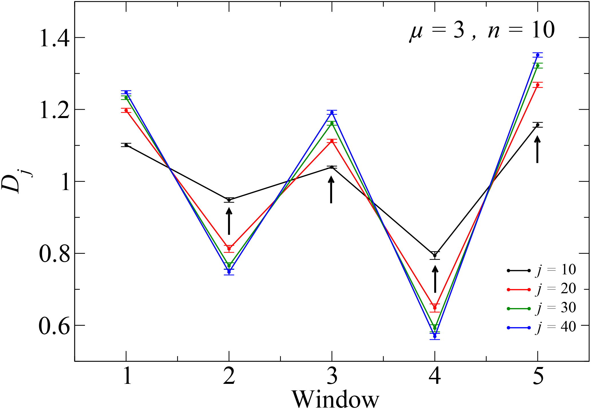
Figure 7 Box-counting fractal dimension for ϵ_b(t) during quiet and active states for n=10, with μ=3. Active states correspond to states labeled “2” and “4”. (Taken from Domínguez et al., 2017.)

As observed in Fig. 7, in Fig. 8 we also find lower fractal dimensions for active states than for quiet states. However, this does not hold for arbitrarily large values of j (see Figs. 6 and 7 in Domínguez et al., 2017). We only find it for j>1, but for values that are not too large, suggesting that it is within this range of values of j where the box-counting fractal dimension has statistical information on the dissipative events in the time series. This, in turn, suggests that the findings in Sect. 3 and Domínguez et al. (2014) are not trivial.

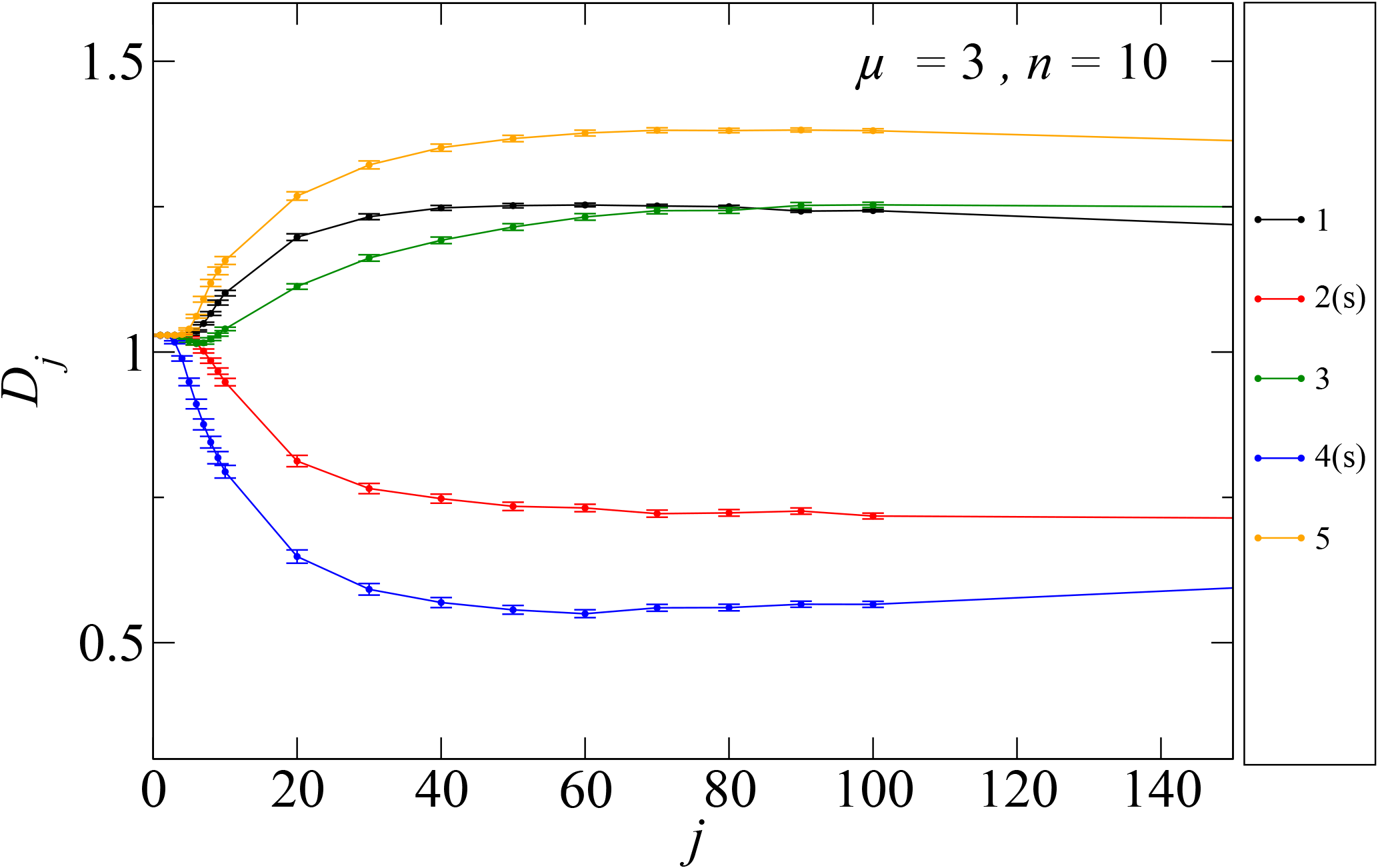
Figure 8 Box-counting fractal dimension for quiet and active states, as a function of j, with μ=3. Numbers for each curve label the states. We added an “(s)” in the legends, in order to highlight the active states. (Taken from Domínguez et al., 2017.)

In Domínguez et al. (2017) a more detailed analysis is carried out on the shell model results, exploring other simulation parameters (ν, η, magnetic Prandtl number), another criterion for defining active states (n=5), and a systematic study of the correlations between the fractal dimension and the occurrence of dissipative events by means of the Student's t-test. Results suggest that the intermittency level of the output time series is relevant, which has led us to perform the analyses for the shell model within a certain range of values of the magnetic Prandtl number, as well as of the viscosity and resistivity.

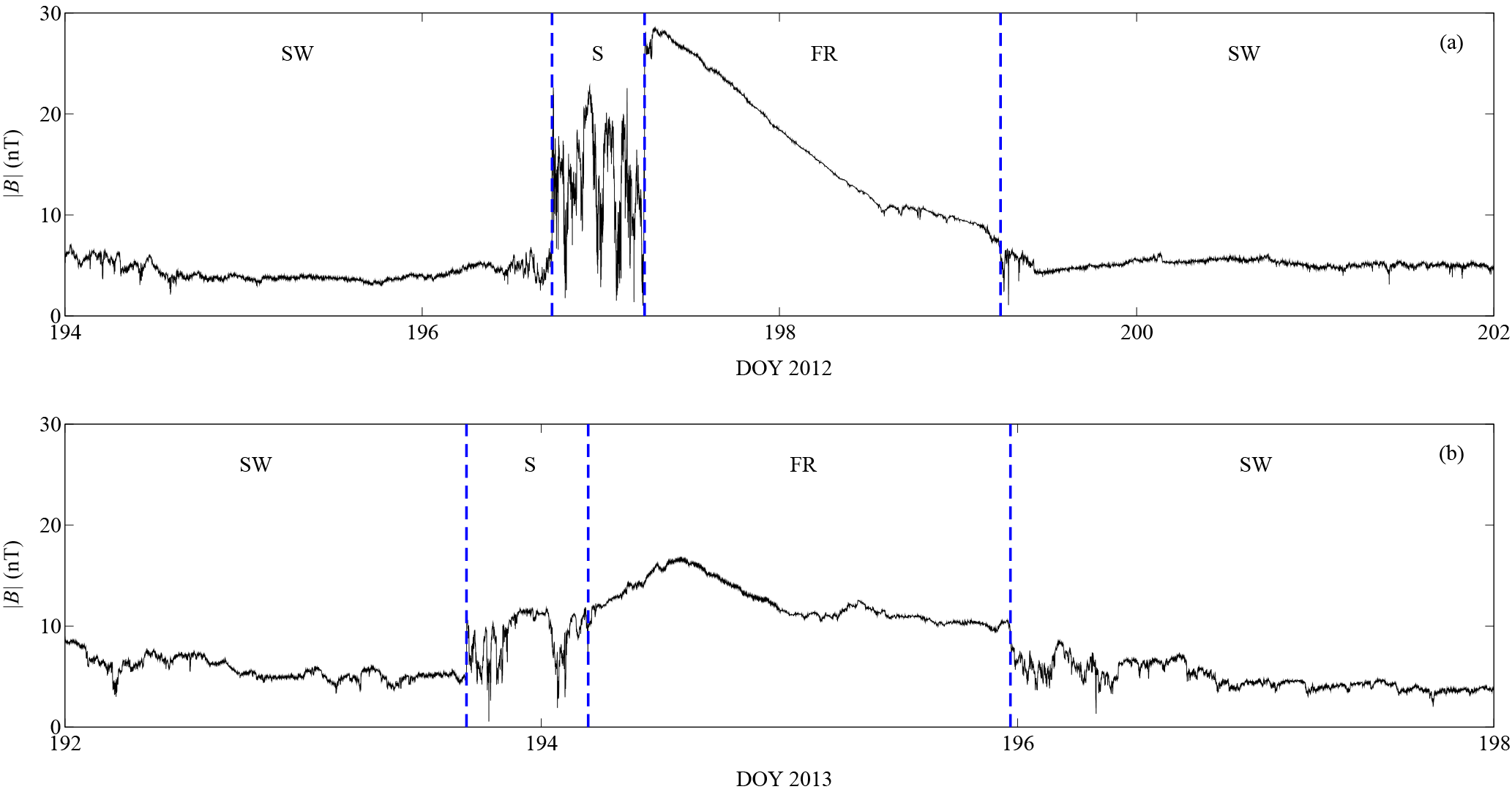
Figure 9 Time series for the magnetic field for the two magnetic cloud events analyzed. The different stages in the data are identified: solar wind (SW), sheath (S), and flux rope (FR). (a) MC1 event: 12 July 2012; (b) MC2 event: 11 July 2013.

5 Magnetic clouds

As a way to illustrate how the ideas described so far could be used to characterize structures in space plasmas, we apply the method to study the time series for the magnetic field during magnetic clouds (Burlaga et al., 1981), as found in ACE interplanetary magnetic field data (ACE Science Center, http://www.srl.caltech.edu/ACE/ASC/index.html) and measured in the proximity of the L1 Lagrangian point. Magnetic clouds are transient structures ejected from the Sun, characterized by a large and smooth rotation of the magnetic field. Typically, a magnetic cloud event can be identified from single spacecraft measurements by studying the evolution of the observed fields. During a given event, various stages can be identified: first, observation of solar wind prior to the cloud's arrival, then a sheath of compressed solar wind plasma immediately preceding a flux rope, where the magnetic field varies smoothly, and finally the background solar wind again. Note that slower moving clouds traveling at speeds comparable to that of the ambient solar wind will not display prominent sheath regions.

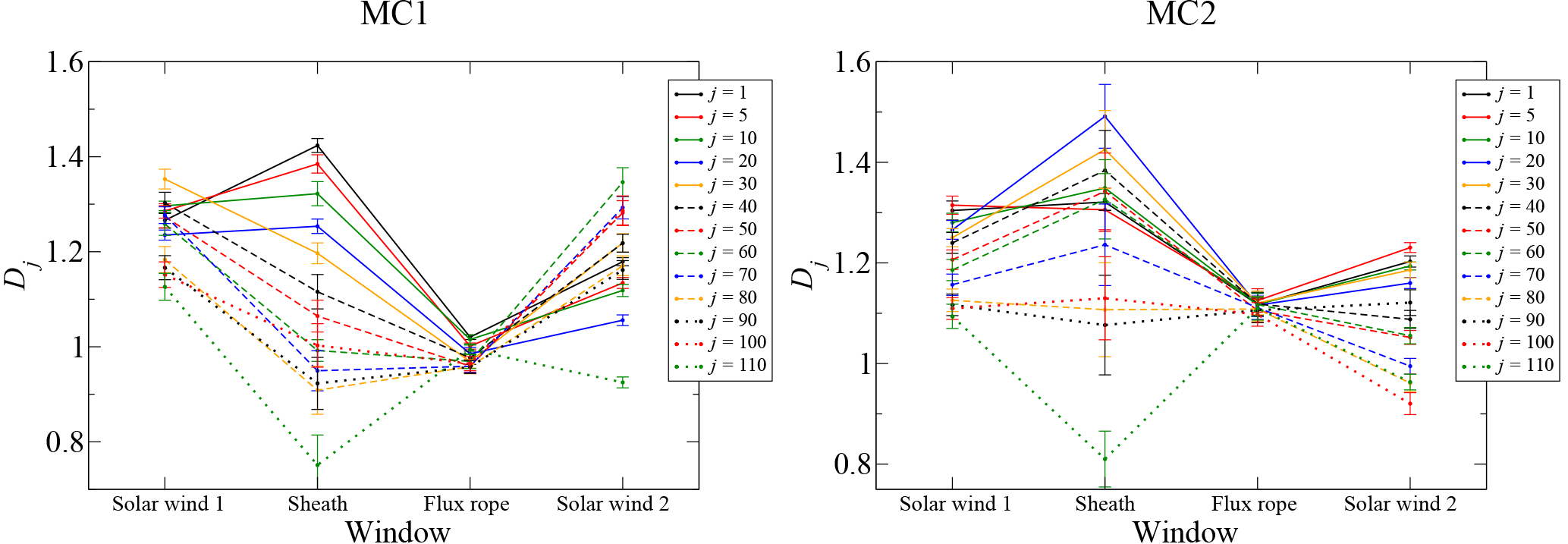
Figure 10 Box-counting fractal dimension for two magnetic cloud events during the four stages of the time series: first the solar wind, then the sheath, then the flux rope, and finally the solar wind again. Several values for data sampling j are used.

Two events were selected: an event occurring on 12 July 2012 (MC1) and another on 11 July 2013 (MC2). Resolution for the magnetic field time series for these events is 16 s, covering a time span of 8 days for MC1 and 6 days for MC2, of which about 2 days correspond to the cloud events themselves.

Figure 9 shows the time series corresponding to the two events analyzed, with the various stages marked.

It is found that the calculated fractal dimension evolves in a distinctive way through the various stages of the event as it passes by the spacecraft (namely surrounding solar wind, sheath, and flux rope). Given the high resolution of the data, it is possible to calculate the box-counting dimension for several delays, given by j, as was shown in Figs. 7 and 8 for the shell model analysis. In Fig. 10 the fractal dimension is calculated for each magnetic cloud stage, and various values of the sampling j are considered.

It can be noted that the fractal dimension, as calculated here, is indeed able to characterize magnetic cloud structures. The sheath state has a large dispersion of fractal dimension values as j is varied, consistent with its more turbulent regime; on the other hand, the quieter and more organized flux rope state exhibits a very low variation with j, basically a single fractal dimension at all timescales explored. As for the surrounding solar wind, it shows dispersion of D_j, which is between the dispersion of values in the sheath and the flux rope.

The results above suggest that, from the point of view of the time series, the level of multifractality is large in the sheath, consistent with its more turbulent nature, intermediate in the solar wind, and that the flux rope magnetic field is essentially monofractal, consistent with the organized, smoother structure of the magnetic field expected in this region. We plan to carry out other multifractal analyses to complement these findings in a future publication.

Also, these results suggest that the fractal approach discussed in this paper may be useful to characterize the various stages of magnetic clouds, and in particular to set up a system to automatically identify similar magnetic structures in spacecraft data.

6 Conclusions

In this paper, we have reviewed recent results obtained by us, regarding the evolution of complexity in magnetized plasmas, as described by geomagnetic data, simulation results for MHD turbulence, and spacecraft data in the solar wind.

This has been done by calculating a box-counting fractal dimension for time series of magnetic field data for the Dst geomagnetic index (Domínguez et al., 2014), the GOY shell model (Domínguez et al., 2017), and ACE data for two magnetic cloud events.

In general, it is found that the fractal dimension D decreases during dissipative events. In the case of the Dst time series this was verified for three different types of time windows: fixed width and stationary, variable width, and moving windows (Sect. 3). And it was also found across several timescales, namely individual storms, full years, and the complete 23rd solar cycle, as detailed in Domínguez et al. (2014).

A similar behavior is found for the MHD shell model (Sect. 4). Thanks to the larger resolution of the simulation data as compared with the Dst data, several values of the time delay for data sampling could be found, showing that the results found in Domínguez et al. (2014) are nontrivial, in the sense that not all samplings yield similar results. Only intermediate values of the time delay that are not too large (as represented by the value of j in Sect. 2) are able to clearly distinguish between active and quiet states. But, within the useful range of values for j, the fractal dimension of the active states is consistently smaller than the dimension of quiet states, and is always lower than 1, whereas the active states always have a dimension larger than 1. The dependence on j of the fractal dimension is interesting in itself, as it suggests that data have a multifractal structure, which is consistent with suggestions and findings by other authors studying space plasmas (Chapman et al., 2008, 1998; Valdivia et al., 2005).

Also, a more systematic test for the correlation between burst events in the shell model and the decrease in fractal dimension was performed, by means of the Student's t-test, as well as a more detailed exploration of the parameter space for the simulation. These results can be found in Domínguez et al. (2017).

As an application of these ideas, we take two magnetic cloud events in the solar wind, and use the techniques described here to study the corresponding magnetic field time series. Our results, although preliminary, suggest that this method can characterize the various stages of the magnetic cloud structure.

Given the rich and complex dynamics governing the evolution of magnetized plasmas, we would not expect that a single index would be able to capture all their relevant information. In fact, multifractal analysis should be conducted in order to represent the dynamics of the systems studied more accurately, and such an analysis is currently being prepared for future publication. However, the findings summarized here suggest that some relevant correlations can be observed, and that the dimension used here, although simple, may give some insight into the evolution of complexity of plasmas in the Sun–Earth system and MHD turbulent states.