Quantum data assimilation: a new approach to solving data assimilation on quantum annealers

Data assimilation is a crucial component in the Earth science field, enabling the integration of observation data with numerical models. In the context of numerical weather prediction (NWP), data assimilation is particularly vital for improving initial conditions and subsequent predictions. However, the computational demands imposed by conventional approaches, which employ iterative processes to minimize cost functions, pose notable challenges in computational time. The emergence of quantum computing provides promising opportunities to address these computation challenges by harnessing the inherent parallelism and optimization capabilities of quantum annealing machines.

In this investigation, we propose a novel approach termed quantum data assimilation, which solves the data assimilation problem using quantum annealers. Our data assimilation experiments using the 40-variable Lorenz model were highly promising, showing that the quantum annealers produced an analysis with comparable accuracy to conventional data assimilation approaches. In particular, the D-Wave Systems physical quantum annealing machine achieved a significant reduction in execution time.

1 Introduction

Data assimilation is a mathematical discipline that integrates numerical models and observation data to improve the interpretation and predictions of dynamical systems (Reichle, 2008; Evensen, 2009). In particular, data assimilation has been intensively investigated in numerical weather prediction (NWP) during the past 2 decades to provide optimal initial conditions by combining model forecasts and observation data (Kalnay, 2003; Houtekamer and Zhang, 2016). Among data assimilation methods, variational and ensemble–variational data assimilation methods, which iteratively reduce cost functions via gradient-based optimization, are widely used in most operational NWP centers such as the European Centre for Medium-Range Weather Forecasts (ECMWF), the United Kingdom Met Office (Met Office), the National Oceanic, Atmospheric Administration of the United States (NOAA) and the Japan Meteorological Agency (JMA). However, data assimilation methods require vast computational resources in NWP systems because of the iterations needed for sufficient cost function reduction. For example, in JMA's global forecast system, data assimilation requires about 25 times more computational resources than forecast computations.

In recent years, quantum computing has attracted research interest as a new paradigm of computational technologies since it has a large potential to overcome computational challenges of conventional approaches through quantum effects such as tunneling, superposition and entanglement. In particular, quantum annealing machines (Kadowaki and Nishimori, 1998), such as D-Wave Systems quantum annealers (Johnson et al., 2011), are powerful and feasible tools for solving optimization problems. Since the quantum annealer 2000Q was released by D-Wave Systems in 2017, quantum computing research has rapidly progressed in various applications, such as for machine learning (Hu et al., 2019; Willsch et al., 2020), graph partitioning (Ushijima-Mwesigwa et al., 2017), clustering (O'Malley et al., 2018), and model predictive control (Inoue et al., 2021).

In this study, we design a data assimilation method for the quantum annealing machines. Although quantum machines have been used in several engineering applications, to our knowledge, this is the first study to apply quantum annealing to data assimilation problems. We focus on the four-dimensional variational data assimilation (4DVAR) since it is the most widely used data assimilation method in operational NWP systems. We reformulate 4DVAR into a quadratic unconstrained binary optimization (QUBO) problem, which can be solved by quantum annealers. We subsequently apply the proposed method for a series of 4DVAR experiments using a low-dimensional chaotic Lorenz 96 model (Lorenz, 1996; Lorenz and Emanuel, 1998), which has been widely used in theoretical data assimilation studies (e.g., Anderson, 2011; Whitaker and Hamill, 2002; Miyoshi, 2011; Kotsuki et al., 2017).

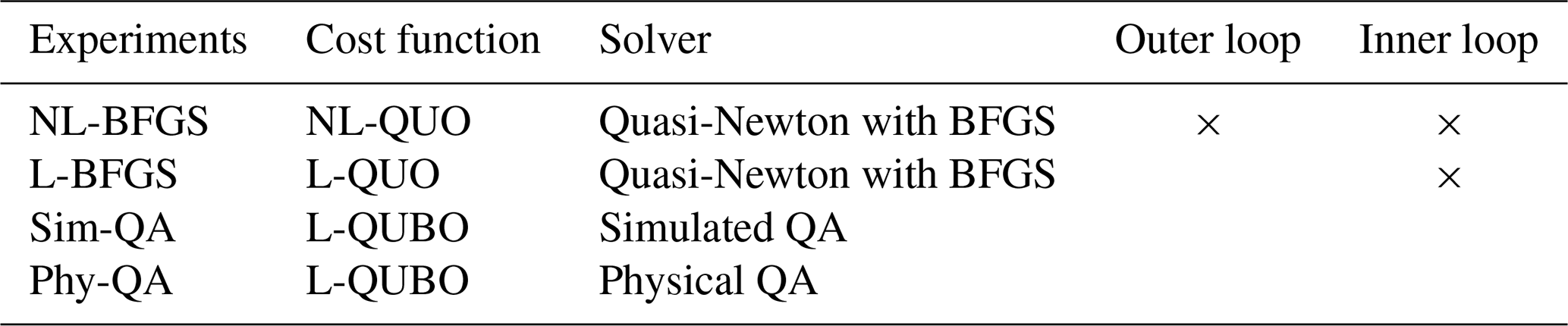
The original 4DVAR cost function is, as elaborated in Sect. 2.1, a quadratic unconstrained optimization (QUO) problem including a nonlinear operator with respect to the analysis increment (NL-QUO). To solve 4DVAR using quantum annealers, we first approximate the problem so as to include only linear operations with respect to the analysis (L-QUO), which is then reformulated to a be quadratic unconstrained binary optimization (L-QUBO) problem. The L-QUBO problem is solved using the D-Wave Advantage physical quantum annealer (Phy-QA) and the Fixstars Amplify simulated quantum annealer (Sim-QA). We also employ the conventionally used quasi-Newton method with the Broyden–Fletcher–Goldfarb–Shanno formula (BFGS) to solve the NL-QUO and L-QUO, which are denoted as NL-BFGS and L-BFGS hereafter. Numerical techniques and practical implementations specifically tailored to quantum data assimilation are also presented.

The rest of paper is organized as follows. Section 2 provides the method of quantum data assimilation, and Sect. 3 provides results and discussion. Finally, a summary is presented in Sect. 4.

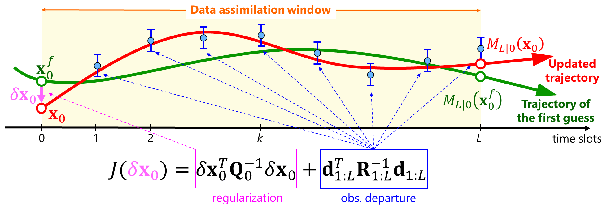
Figure 1 Conceptual image of 4DVAR data assimilation. Green and red lines indicate the trajectories of the first guess and updated analysis, respectively. Blue circles with error bars represent observations.

2 Methodology and experiments

2.1 Conventional data assimilation

This study focuses on the four-dimensional variational data assimilation (4DVAR), which is among the most widely used data assimilation methods in operational NWP centers such as ECMWF, Met Office, NOAA, and JMA. 4DVAR assimilates observations over a time window to produce an analysis trajectory that minimizes its cost function (Fig. 1). The cost function of 4DVAR is derived from Bayes' theorem and is given by

$$\begin{array}{}\text{(1)}& J\left(\mathit{\delta }{\mathbf{x}}_{\mathrm{0}}\right)=\mathit{\delta }{\mathbf{x}}_{\mathrm{0}}^T{\mathbf{Q}}_{\mathrm{0}}^{-\mathrm{1}}\mathit{\delta }{\mathbf{x}}_{\mathrm{0}}+{\mathit{d}}_{\mathrm{1}:L}^T{\mathbf{R}}_{\mathrm{1}:L}^{-\mathrm{1}}{\mathit{d}}_{\mathrm{1}:L},\end{array}$$

where $\mathit{\delta }{\mathbf{x}}_{\mathrm{0}}={\mathbf{x}}_{\mathrm{0}}-{\mathbf{x}}_{\mathrm{0}}^{\mathrm{f}}$ (∈R^N) is the analysis increment, Q ($\in R^{N\times N}$) is the background error covariance, d_1:L (∈R^PL) is the observation departure, and R_1:L ($\in R^{PL\times PL}$) is the observation error covariance. The superscript f represents the forecast, the subscript 0 denotes time t=0 of the time window, and 1:L indicates observation time slots from t=1 to t=L. Here, N is the system size, L is the number of observation time slots, and P is the number of observations per time slot. The observation departure is given by

$$\begin{array}{}\text{(2)}& {\displaystyle }{\mathit{d}}_{\mathrm{1}:L}^T=\left[{\mathit{d}}_{\mathrm{1}}^T,\mathrm{\dots },{\mathit{d}}_k^T,\mathrm{\dots },{\mathit{d}}_L^T\right],\text{(3)}& {\displaystyle }{\mathit{d}}_k={\mathbf{y}}_k^{\mathrm{o}}-\mathbf{H}{M}_{k\mathrm{|}\mathrm{0}}\left({\mathbf{x}}_{\mathrm{0}}^{\mathrm{f}}+\mathit{\delta }{\mathbf{x}}_{\mathrm{0}}\right),\end{array}$$

where ${\mathbf{y}}_k^{\mathrm{o}}$ (∈R^P) is the observation at time k, and M_k|0() is the nonlinear model forecast from time t=0 to k, and H ($\in R^{P\times N}$) is the linear observation operator. The superscript o denotes the observation. Conventional 4DVAR iteratively updates the analysis increment, δx₀, by reducing the cost function using the quasi-Newton method based on the gradient

$$\begin{array}{}\text{(4)}& \partial J\left(\mathit{\delta }{\mathbf{x}}_{\mathrm{0}}\right)/\partial \mathit{\delta }{\mathbf{x}}_{\mathrm{0}}=\mathrm{2}{\mathbf{Q}}_{\mathrm{0}}^{-\mathrm{1}}\mathit{\delta }{\mathbf{x}}_{\mathrm{0}}-\mathrm{2}{\mathbf{M}}_{\mathrm{1}:L}^T{\mathbf{H}}_{\mathrm{1}:L}^T{\mathbf{R}}_{\mathrm{1}:L}^{-\mathrm{1}}{\mathit{d}}_{\mathrm{1}:L},\end{array}$$

where

$$\begin{array}{}\text{(5)}& {\mathbf{H}}_{\mathrm{1}:L}^T=\left[\begin{array}{ccc}{\mathbf{H}}^T& & \mathbf{O}\\ & \mathrm{\ddots }& \\ \mathbf{O}& & {\mathbf{H}}^T\end{array}\right]\end{array}$$

and O is the zero matrix. The adjoint model ${\mathbf{M}}_{\mathrm{1}:L}^T$ ($\in R^{N\times NL}$) is given by

$$\begin{array}{}\text{(6)}& {\displaystyle }{\mathbf{M}}_{\mathrm{1}:L\mathrm{|}\mathrm{0}}^T=\left[{\mathbf{M}}_{\mathrm{1}\mathrm{|}\mathrm{0}}^T,\mathrm{\dots },{\mathbf{M}}_{k\mathrm{|}\mathrm{0}}^T,\mathrm{\dots },{\mathbf{M}}_{L\mathrm{|}\mathrm{0}}^T\right],\text{(7)}& {\displaystyle }{\mathbf{M}}_{k\mathrm{|}\mathrm{0}}^T={\prod }_{l=\mathrm{1}}^k{\mathbf{M}}_{l\mathrm{|}l-\mathrm{1}}^T,\end{array}$$

where M_l|l−1 ($\in {\mathrm{R}}^{N\times N}$) is the tangent liner model that approximates

$$\begin{array}{}\text{(8)}& \begin{array}{rl}{M}_{l\mathrm{|}l-\mathrm{1}}& \left(M_{l-\mathrm{1}\mathrm{|}\mathrm{0}}\left({\mathbf{x}}_{\mathrm{0}}^{\mathrm{f}}+\mathit{\delta }{\mathbf{x}}_{\mathrm{0}}\right)+\mathit{\epsilon }\right)\\ & \simeq M_{l\mathrm{|}\mathrm{0}}\left({\mathbf{x}}_{\mathrm{0}}^{\mathrm{f}}+\mathit{\delta }{\mathbf{x}}_{\mathrm{0}}\right)+{\mathbf{M}}_{l\mathrm{|}l-\mathrm{1}}\mathit{\epsilon },\end{array}\end{array}$$

where ε (∈R^N) is the vector with very small real numbers and $\mathit{\epsilon }={\mathrm{10}}^{-\mathrm{5}}\times {\left[\mathrm{1},\mathrm{\cdots },\mathrm{1}\right]}^T$ is used in this study. This optimization minimizes the quadratic cost function (Eq. 1), including the nonlinear operator with respect to the analysis increment (Eq. 3), and is referred to as NL-QUO in this study. In NL-QUO, the tangent linear model, M, and its adjoint model, M^T, are updated at every iteration based on the latest analysis; ${\mathbf{x}}_{\mathrm{0}}={\mathbf{x}}_{\mathrm{0}}^{\mathrm{f}}+\mathit{\delta }{\mathbf{x}}_{\mathrm{0}}$.

As an intermediate step toward QUBO, the original cost function is approximated as follows:

$$\begin{array}{}\text{(9)}& J\left(\mathit{\delta }{\mathbf{x}}_{\mathrm{0}}\right)\simeq \stackrel{\mathrm{̃}}{J}\left(\mathit{\delta }{\mathbf{x}}_{\mathrm{0}}\right)=\mathit{\delta }{\mathbf{x}}_{\mathrm{0}}^T{\mathbf{Q}}_{\mathrm{0}}^{-\mathrm{1}}\mathit{\delta }{\mathbf{x}}_{\mathrm{0}}+{\stackrel{\mathrm{̃}}{\mathit{d}}}_{\mathrm{1}:L}^T{\mathbf{R}}_{\mathrm{1}:L}^{-\mathrm{1}}{\stackrel{\mathrm{̃}}{\mathit{d}}}_{\mathrm{1}:L},\end{array}$$

where

$$\begin{array}{}\text{(10)}& {\displaystyle }{\stackrel{\mathrm{̃}}{\mathit{d}}}_{\mathrm{1}:L}^T=\left[{\stackrel{\mathrm{̃}}{\mathit{d}}}_{\mathrm{1}}^T,\mathrm{\dots },{\stackrel{\mathrm{̃}}{\mathit{d}}}_k^T,\mathrm{\dots },{\stackrel{\mathrm{̃}}{\mathit{d}}}_L^T\right],\text{(11)}& {\displaystyle }{\mathit{d}}_k\simeq {\stackrel{\mathrm{̃}}{\mathit{d}}}_k={\mathbf{y}}_k^{\mathrm{o}}-{\mathbf{Hx}}_k^{\mathrm{f}}-\mathbf{H}{\stackrel{\mathrm{̃}}{\mathbf{M}}}_{k\mathrm{|}\mathrm{0}}\mathit{\delta }{\mathbf{x}}_{\mathrm{0}},\text{(12)}& {\displaystyle }{\stackrel{\mathrm{̃}}{\mathbf{M}}}_{k\mathrm{|}\mathrm{0}}={\prod }_{l=\mathrm{0}}^{k-\mathrm{1}}{\stackrel{\mathrm{̃}}{\mathbf{M}}}_{l\mathrm{|}l-\mathrm{1}}.\end{array}$$

Here, ${\mathbf{x}}_k^{\mathrm{f}}=M_{k\mathrm{|}\mathrm{0}}\left({\mathbf{x}}_{\mathrm{0}}^{\mathrm{f}}\right)$, and the tilde indicates linear approximations. Unlike NL-QUO, this optimization retains the same tangent linear model and its adjoint model during the iteration. Namely, the tangent linear model is expanded not around the trajectory from the latest analysis (${\mathbf{x}}_{\mathrm{0}}^{\mathrm{f}}+\mathit{\delta }{\mathbf{x}}_{\mathrm{0}}$) but around the trajectory from the first guess (${\mathbf{x}}_{\mathrm{0}}^{\mathrm{f}}$) as follows:

$$\begin{array}{}\text{(13)}& M_{l\mathrm{|}l-\mathrm{1}}\left(M_{l-\mathrm{1}\mathrm{|}\mathrm{0}}\left({\mathbf{x}}_{\mathrm{0}}^{\mathrm{f}}\right)+\mathit{\epsilon }\right)\simeq M_{l\mathrm{|}\mathrm{0}}\left({\mathbf{x}}_{\mathrm{0}}^{\mathrm{f}}\right)+{\stackrel{\mathrm{̃}}{\mathbf{M}}}_{l\mathrm{|}l-\mathrm{1}}\mathit{\epsilon }.\end{array}$$

The substitution of Eqs. (10)–(12) into Eq. (9) gives the following quadratic unconstraint optimization (L-QUO) that has only linear operations with respect to the analysis increment as follows:

$$\begin{array}{}\text{(14)}& \begin{array}{rl}\stackrel{\mathrm{̃}}{J}\left(\mathit{\delta }{\mathbf{x}}_{\mathrm{0}}\right)& =\mathit{\delta }{\mathbf{x}}_{\mathrm{0}}^T\left({\mathbf{Q}}_{\mathrm{0}}^{-\mathrm{1}}+{\stackrel{\mathrm{̃}}{\mathbf{M}}}_{\mathrm{1}:L\mathrm{|}\mathrm{0}}^T{\mathbf{H}}_{\mathrm{1}:L}^T{\mathbf{R}}_{\mathrm{1}:L}^{-\mathrm{1}}{\mathbf{H}}_{\mathrm{1}:L}{\stackrel{\mathrm{̃}}{\mathbf{M}}}_{\mathrm{1}:L\mathrm{|}\mathrm{0}}\right)\\ & \cdot \mathit{\delta }{\mathbf{x}}_{\mathrm{0}}-\mathrm{2}{\mathbf{s}}_{\mathrm{1}:L}^T{\mathbf{R}}_{\mathrm{1}:L}^{-\mathrm{1}}{\mathbf{H}}_{\mathrm{1}:L}{\stackrel{\mathrm{̃}}{\mathbf{M}}}_{\mathrm{1}:L\mathrm{|}\mathrm{0}}\mathit{\delta }{\mathbf{x}}_{\mathrm{0}}+C,\end{array}\end{array}$$

where the constant C is

$$\begin{array}{}\text{(15)}& {\displaystyle }C={\mathbf{s}}_{\mathrm{1}:L}^T{\mathbf{R}}_{\mathrm{1}:L}^{-\mathrm{1}}{\mathbf{s}}_{\mathrm{1}:L},\text{(16)}& {\displaystyle }{\mathbf{s}}_{\mathrm{1}:L}^T=\left[{\mathbf{s}}_{\mathrm{1}}^T,\mathrm{\dots },{\mathbf{s}}_k^T,\mathrm{\dots },{\mathbf{s}}_L^T\right],\text{(17)}& {\displaystyle }{\mathbf{s}}_k={\mathbf{y}}_k^{\mathrm{o}}-{\mathbf{Hx}}_k^{\mathrm{f}}.\end{array}$$

The gradient of $\stackrel{\mathrm{̃}}{J}$ is given by

$$\begin{array}{}\text{(18)}& \begin{array}{rl}{\displaystyle \frac{\partial \stackrel{\mathrm{̃}}{J}\left(\mathit{\delta }{\mathbf{x}}_{\mathrm{0}}\right)}{\partial \mathit{\delta }{\mathbf{x}}_{\mathrm{0}}}}& =\mathrm{2}\left({\mathbf{Q}}_{\mathrm{0}}^{-\mathrm{1}}+{\stackrel{\mathrm{̃}}{\mathbf{M}}}_{\mathrm{1}:L\mathrm{|}\mathrm{0}}^T{\mathbf{H}}_{\mathrm{1}:L}^T{\mathbf{R}}_{\mathrm{1}:L}^{-\mathrm{1}}{\mathbf{H}}_{\mathrm{1}:L}{\stackrel{\mathrm{̃}}{\mathbf{M}}}_{\mathrm{1}:L\mathrm{|}\mathrm{0}}\right)\\ & \cdot \mathit{\delta }{\mathbf{x}}_{\mathrm{0}}-\mathrm{2}{\stackrel{\mathrm{̃}}{\mathbf{M}}}_{\mathrm{1}:L\mathrm{|}\mathrm{0}}^T{\mathbf{H}}_{\mathrm{1}:L}^T{\mathbf{R}}_{\mathrm{1}:L}^{-\mathrm{1}}{\mathbf{s}}_{\mathrm{1}:L}.\end{array}\end{array}$$

2.2 Quantum data assimilation

Quantum annealers require only the cost function in contrast to conventional 4DVAR that requires the cost function and its gradient. However, the cost function should be represented by binary variables (i.e., 0 or 1) for quantum annealers. In this study, we represent a real number with Z qubits, where Z is a natural number. In accordance with the method of Inoue et al. (2021), a mapping matrix, G ($\in R^{N\times NZ}$), is used in this study.

$$\begin{array}{}\text{(19)}& {\displaystyle }\mathit{\delta }{\mathbf{x}}_{\mathrm{0}}\simeq {\displaystyle \frac{\mathrm{1}}{\mathit{\alpha }}}\mathbf{G}\mathit{b}={\displaystyle \frac{\mathrm{1}}{\mathit{\alpha }}}\left[\begin{array}{ccc}{\mathbf{g}}^T& & \mathbf{0}\\ & \mathbf{\ddots }& \\ \mathbf{0}& & {\mathbf{g}}^T\end{array}\right]\mathit{b},\text{(20)}& {\displaystyle }{\mathbf{g}}^T=\left[-{\mathrm{2}}^{Z-\mathrm{1}},{\mathrm{2}}^{Z-\mathrm{2}},{\mathrm{2}}^{Z-\mathrm{3}},\mathrm{\dots },{\mathrm{2}}^{\mathrm{1}},{\mathrm{2}}^{\mathrm{0}}\right],\end{array}$$

where α is the tunable scaling parameter, b (∈R^NZ) is the binary vector whose elements are all either 0 or 1, and 0 is the vector whose elements are all 0. Thus, Eq. (14) is reformulated into QUBO as follows:

$$\begin{array}{}\text{(21)}& \stackrel{\mathrm{̃}}{J}\left(\mathit{\delta }{\mathbf{x}}_{\mathrm{0}}\right)\simeq H\left(\mathit{b}\right)={\mathit{b}}^T\mathbf{Ab}+{\mathbf{u}}^T\mathit{b}+C,\end{array}$$

where H is the Hamiltonian. A ($\in R^{NZ\times NZ}$) and u (∈R^NZ) are given as follows:

$$\begin{array}{}\text{(22)}& {\displaystyle }\mathbf{A}={\displaystyle \frac{\mathrm{1}}{{\mathit{\alpha }}^{\mathrm{2}}}}{\mathbf{G}}^T\left({\mathbf{Q}}_{\mathrm{0}}^{-\mathrm{1}}+{\stackrel{\mathrm{̃}}{\mathbf{M}}}_{\mathrm{1}:L\mathrm{|}\mathrm{0}}^T{\mathbf{H}}_{\mathrm{1}:L}^T{\mathbf{R}}_{\mathrm{1}:L}^{-\mathrm{1}}{\mathbf{H}}_{\mathrm{1}:L}{\stackrel{\mathrm{̃}}{\mathbf{M}}}_{\mathrm{1}:L\mathrm{|}\mathrm{0}}\right)\mathbf{G},\text{(23)}& {\displaystyle }{\mathbf{u}}^T=-{\displaystyle \frac{\mathrm{2}}{\mathit{\alpha }}}{\mathbf{s}}_{\mathrm{1}:L}^T{\mathbf{R}}_{\mathrm{1}:L}^{-\mathrm{1}}{\mathbf{H}}_{\mathrm{1}:L}{\stackrel{\mathrm{̃}}{\mathbf{M}}}_{\mathrm{1}:L\mathrm{|}\mathrm{0}}\mathbf{G}.\end{array}$$

Note that the constant C is irrelevant to the minimization problem. Quantum annealers solve the QUBO problem (Eq. 21) by inputting A and u into the solvers.

Table 1 Experiments conducted in this study. Outer loop indicates that the trajectory is updated during 4DVAR. Inner loop indicates that the analysis increments are computed iteratively by the quasi-Newton method with the BFGS formula.

2.3 Experiments with the Lorenz 96 model

This study performs twin idealized experiments using the 40-variable Lorenz 96 model, which has been used widely in theoretical data assimilation studies (e.g., Anderson, 2011; Whitaker and Hamill, 2002; Miyoshi, 2011; Kotsuki et al., 2017). The Lorenz 96 model is defined as follows:

$$\begin{array}{}\text{(24)}& {\displaystyle \frac{\mathrm{d}{x}_i}{\mathrm{d}t}}=\left(x_{i+\mathrm{1}}-x_{i-\mathrm{2}}\right)x_{i-\mathrm{1}}-x_i+F,i=\mathrm{1},\mathrm{2},\mathrm{\dots },N,\end{array}$$

where the boundary is cyclic (i.e., $x_i=x_{i+N}=x_{i-N}$) and the model dimension, N, is 40. The forcing is fixed at F=8.0, which makes the model behave chaotically. The model is integrated using a fourth-order Runge–Kutta scheme with a non-dimensional time step of 0.05. A time step of 0.05 is considered to be 6 h, following Lorenz and Emanuel (1998). This study uses the identity matrix for the observation error covariance such that variance of the uncorrelated observation error is 1.0. We first employed the nature run by running the Lorenz 96 model, and observation data were generated based on the nature run every 6 h (0.05 time units). All grid points are observed. The background error covariance is tuned to be Q=0.15I. As in conventional 4DVAR, NL-QUO and L-QUO are solved using the quasi-Newton method with Broyden–Fletcher–Goldfarb–Shanno (BFGS) formula (Table 1). In our BFGS-based 4DVAR experiments, we use the AMD Ryzen 7 5800U with a Radeon graphics card as the CPU. All source codes are written in the Python v3.8.10. The NumPy and SciPy libraries are used for numerical computations. We first conducted NL-QUO 4DVAR data assimilation cycles 50 times over a period of 100 d, with a 2 d time window. Then, we preserved the 50 pieces of first-guess data, which were subsequently used for the other three approaches: L-QUO by BFGS and L-QUBO by simulated and physical quantum annealers. Namely, our experiments purely compare the optimization processes of data assimilation among the four approaches.

2.4 Quantum annealers

As the experimental environment of the Phy-QA, we use D-Wave Advantage System 4.1 which consists of 5627 physical qubits and 177 logical qubits, respectively (D-Wave, 2022). Because the D-Wave Advantage performs computations using the logical qubits, the 177 logical qubits are available for computations. Because of this limitation, we represent a real number (an analysis increment for one variable of the Lorenz 96 model) with four logical qubits (Z=4) to limit the size of binary vector b less than 177 logical qubits (i.e., $N\times Z=\mathrm{40}\times \mathrm{4}=\mathrm{160}\le \mathrm{177}$). The computational time of the D-Wave optimizations are measured using the execution_time function. Quantum annealers give b as a solution of the QUBO problem by submitting input parameters A and u to the solvers (Eq. 21). Here, it is essential to emphasize that physical quantum annealers do not employ traditional algorithms to solve QUBO problems; instead, they obtain solution b as a result of quantum effects. Additional details on quantum annealers can be found in Appendix A.

For the simulated quantum annealer, we use the Fixstars Amplify simulated quantum annealer (Fixstars Amplify Annealing Engine), which incorporates ≥65 536 physical and logical qubits (Matsuda, 2020). The simulated quantum annealer emulates quantum effects via digital computations using the graphics processing unit (GPU). Although the simulated quantum annealers cannot cause real quantum effects, they are applicable to large-scale calculations due to their logical qubits being larger than those of Phy-QA. The computational time is also measured by the execution_time function for Sim-QA. Despite the larger number of logical qubits available in the Fixstars Amplify Sim-QA, we use four logical qubits for a real number (Z=4) in numerical experiments to compare with the D-Wave Phy-QA. Consequently, we use 160 logical qubits for both of Sim-QA and Phy-QA experiments.

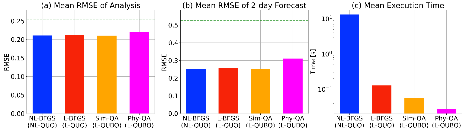
Figure 2 (a) Mean analysis root mean square errors (RMSEs) at the initial time of the 4DVAR data assimilation window (a-RMSE), (b) mean 2 d forecast RMSEs (f-RMSE), and (c) mean execution time (s) over 50 data assimilations for NL-BFGS (a-RMSE = 0.2109; f-RMSE = 0.2520; 13.18 s; blue), L-BFGS (a-RMSE = 0.2120; f-RMSE = 0.2554; 0.129 s; red), Fixstars Amplify Sim-QA (a-RMSE = 0.2105; f-RMSE = 0.2531; 0.057 s; orange), and D-Wave Phy-QA (a-RMSE = 0.2209; f-RMSE = 0.3101; 0.028 s; magenta). The dashed green lines in (a) and (b) indicate the first guess prior to data assimilation (a-RMSE = 0.2530; f-RMSE = 0.5267). The num_reads of Phy-QA was set to 50. The scaling factor, α, was set to 20 and 50 for Sim-QA and Phy-QA, respectively.

3 Results and discussion

3.1 Performance of quantum data assimilation

Figure 2a and b show a comparison of the mean analysis and 2 d forecast root mean square errors (RMSEs) with respect to the nature run for the four different approaches. As anticipated, the NL-BFGS achieved the lower RMSEs as it did not approximate the original cost function. Approximating the nonlinear operations of the original cost function led to a slight increase in the analysis and forecast RMSEs, as observed in L-BFGS. Solving QUBO using the quantum annealers resulted in reduced analysis errors compared to the first guess, as demonstrated by the Sim-QA and Phy-QA. Here, tunable parameters for quantum annealers, namely the scaling factor, α, and num_reads, were calibrated prior to experiments and are discussed in the following subsection (Sect. 3.2). Although Phy-QA successfully reduced analysis errors when compared to the first guess, it exhibited a slightly larger analysis RMSE than the other three approaches. The larger RMSE of Phy-QA is intensified when we see the 2 d forecast RMSE. This discrepancy could be attributed to the stochastic quantum effects inherent in D-Wave's quantum annealer, as discussed in detail in the next subsection.

On the other hand, Phy-QA demonstrated the fastest execution time among the four approaches (Fig. 2c). Here, NL-BFGS exhibited the longest computation time due to the iterative updates of the trajectory and its tangent linear and adjoint models. In contrast, L-BFGS, which retains the first-guess-based trajectory, was significantly faster than NL-BFGS. Sim-QA required a longer execution time than Phy-QA, presumably because GPU-based simulated quantum annealers involve computations for the artificial emulation of quantum effects. The D-Wave Phy-QA obtained a significant reduction in computation time compared to the other three approaches (NL-BFGS, L-BFGS, and Sim-QA), taking less than 0.05 s to find a solution.

It should be noted that there are slight differences in analysis and forecast RMSEs between NL-BFGS and L-BFGS in Fig. 2a and b. The degradations of L-BFGS with respect to NL-BFGS would be more pronounced for stronger nonlinear cases, such as those with longer time windows of 4DVAR, since Eqs. (9)–(13) directly simplify the nonlinear operator in 4DVAR to a linear operator. Here, our quantum data assimilation solves the QUBO problem (Eq. 21), which is an approximation of the cost function solved in L-BFGS (Eq. 14). Therefore, Sim-QA and Phy-QA would worsen too for stronger nonlinear cases.

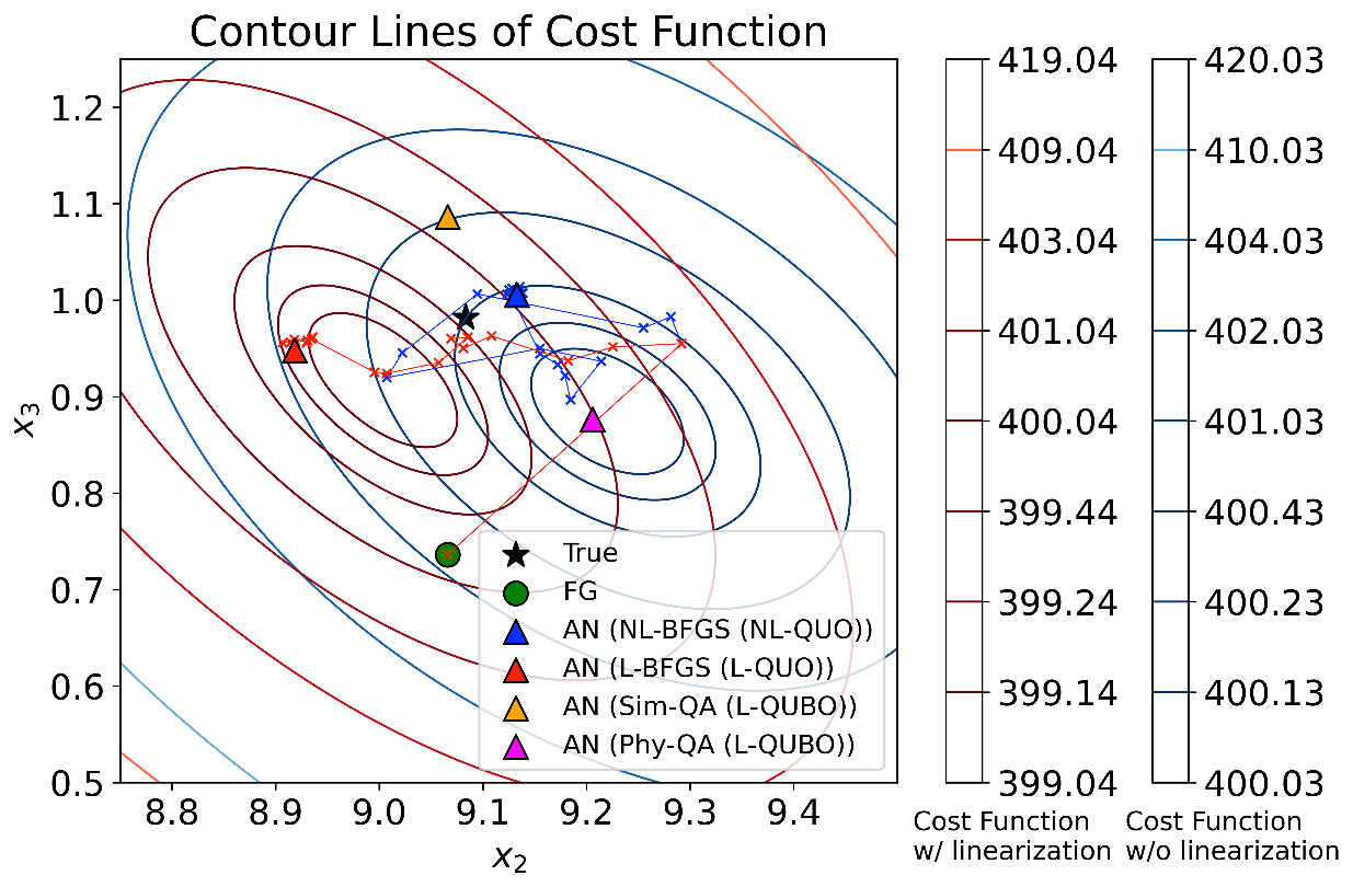
Figure 3 An illustration of data assimilations from an arbitrarily selected first guess. The black star and the green circle indicate the truth and the first guess, respectively. Blue, red, orange, and magenta triangles are the analyses of NL-BFGS, L-BFGS, Sim-QA, and Phy-QA, respectively. Blue and red lines represent the analysis updates over iterations for NL-BFGS and L-BFGS, whose internal analyses are indicated by the cross marks. Red and blue contours show the cost functions with and without the linearization (L-QUO and NL-QUO), respectively. These cost functions were computed in a grid search for 2 variables (x₂ and x₃) of the Lorenz 96 model, with true data used for the other 38 variables. Since the BFGS-based 4DVAR algorithm updates 40 variables, analyses of NL-QUO and L-QUO (blue and red circles) are not exactly placed at the minima of their cost functions. The num_reads of Phy-QA was set to 50. The scaling factor α was set to 20 and 50 for Sim-QA and Phy-QA, respectively.

Figure 3 provides an arbitrarily selected data assimilation example, where the cost functions of NL-QUO and L-QUO are depicted by blue and red contour lines, respectively. Note that Fig. 3 shows an example of analysis while Fig. 2a provides the mean RMSEs averaged over 50 data assimilations. The BFGS-based 4DVAR (NL-BFGS and L-BFGS) gradually converged towards their respective analyses through iterative updates. Consequently, both NL-BFGS and L-BFGS yielded analyses that are closer to the minima of their respective cost functions compared to the first guess (blue and red triangles in Fig. 3). In contrast, Sim-QA and Phy-QA produced a single analysis each as they do not involve iterations. In this specific example, Sim-QA, aiming to minimize L-QUBO, generated an analysis (as a yellow triangle) that was distant from the bottom of L-QUO. Conversely, the analysis produced by Phy-QA (a magenta triangle) is closer to the minima of NL-QUO. Notably, despite solving the same L-QUBO problem, Sim-QA and Phy-QA yielded greatly different analyses in this example. This discrepancy is presumed to be a result of stochastic quantum effects, which will be further investigated in the next subsection.

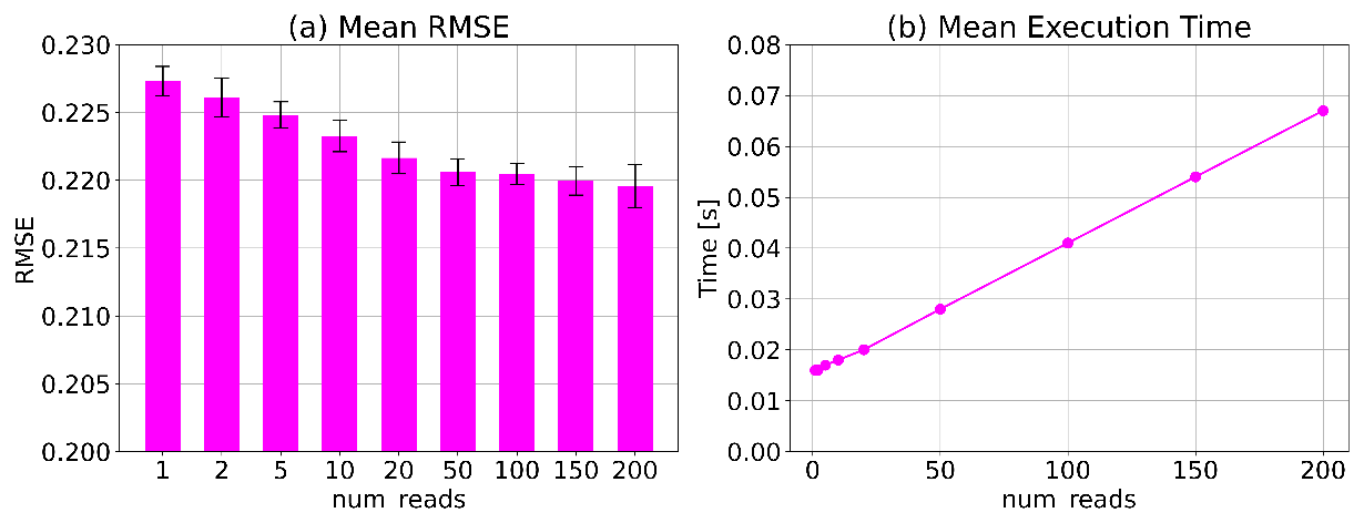
Figure 4 Sensitivity of (a) analysis RMSE and (b) mean execution time to the tunable parameter num_reads in D-Wave Phy-QA. We conducted 50 data assimilations 10 times, and their means and standard deviations over 10 samples are represented by bars and error bars. The scaling factor α is set to 50.

3.2 Sensitivity to tunable parameters

It is important to mention that the D-Wave physical quantum annealer produces non-deterministic outputs due to stochastic quantum effects. Therefore, the quantum annealer includes a tunable parameter called num_reads, which defines the number of states (output solutions) to be read from the solver. Generally, a larger value of num_reads increases the probability of obtaining a better solution. Here, the better solution, which results in smaller Hamiltonian H (Eq. 21), is expected to yield smaller analysis RMSEs. In this study, we investigated the sensitivity of Phy-QA to the num_reads parameter. Figure 4 illustrates the sensitivity of the analysis RMSE and the mean computational time with respect to the num_reads parameter. For each num_reads value, we repeated 50 data assimilations 10 times. The mean RMSE and standard deviation over the 10 samples are presented in Fig. 4a. Increasing the value of num_reads generally resulted in a reduction in the analysis RMSE. While the execution time exhibited a linear increase with respect to num_reads (Fig. 4b), reading out solutions from the solver multiple times proved beneficial in achieving stable and improved analyses. Importantly, the standard deviation of the mean RMSE was found to be insensitive to the num_reads parameter. This observation indicates that even if we read out the output from the solver over 100 times, the stochastic effects persist and cannot be eliminated for Phy-QA.

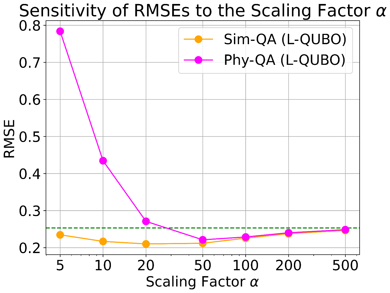
Figure 5 Sensitivity of analysis RMSEs to the scaling factor α for Sim-QA (orange) and Phy-QA (magenta). The dashed green line in (a) represents the first-guess RMSE prior to data assimilation. The parameter num_reads of Phy-QA is set to 50.

The scaling factor α is an important parameter for regulating analysis accuracy in quantum annealers (see Eq. 19). Due to the limited number of available logical qubits for Phy-QA, this study represented real numbers using only four logical qubits. In other words, both our Phy-QA and Sim-QA could only represent 2⁴=16 distinct real numbers. For instance, a scaling factor of α=20 indicates that numerical experiments can handle real numbers ranging from −0.40 to 0.35 in increments of 0.05. Our sensitivity experiments to the scaling factor, α, revealed similar increasing trends for Phy-QA and Sim-QA when α≥50 (Fig. 5). Increasing the scaling factor, α, resulted in degraded analysis accuracy, approaching the RMSE of the first guess. This is because excessively large scaling factors can lead to slight changes in the analysis increment. For instance, when α=500, the minimum and maximum analysis increments are −0.016 and 0.014, respectively. It indicates that when α=500, Phy-QA and Sim-QA can manage a limited increment (from −0.016 to 0.014); as a result, their RMSEs approach the RMSE of the first guess. Interestingly, noticeable discrepancies were observed between Phy-QA and Sim-QA for α≤20, presumably due to the stochastic quantum effects specific to Phy-QA. As observed in Fig. 4, we cannot eliminate stochastic effects for Phy-QA even if we read out output from the solver over 100 times. For smaller scaling factors, a stochastic change in a single qubit can induce larger changes in the analysis increment. Consequently, the optimal scaling factor for Phy-QA was found to be larger than that for Sim-QA. Based on the results of the sensitivity experiments, scaling factors of α=20 and α=50 were used for Sim-QA and Phy-QA in Sect. 3.1. These sensitivity experiments also indicate that the optimal scaling factor may differ between Sim-QA and Phy-QA.

4 Summary

This study proposed the quantum data assimilation which solves data assimilation problems on quantum annealing machines. The main results of this investigation are as follows:

1. We reformulated the data assimilation problem into the quadratic unconstrained binary optimization (QUBO) problem so that quantum annealing machines can solve data assimilation.

2. Using the 40-variable Lorenz model, we succeeded in solving data assimilation on quantum annealers for the first time. The results of our experiments were highly promising, demonstrating that the quantum annealers can yield an analysis whose accuracy is comparable to the conventional quasi-Newton-based iterative approach.

3. The D-Wave physical quantum annealing machine needed an execution time of less than 0.05 s, which is significantly smaller than conventional approaches.

4. Since the D-Wave physical quantum annealer produces non-deterministic outputs due to stochastic quantum effects, reading out solutions multiple times was beneficial in achieving stable and improved analyses.

5. The scaling factor for quantum data assimilation is an important parameter for regulating analysis accuracy in our configuration. Due to the stochastic quantum effects, the optimal scaling factor for D-Wave's physical quantum annealing machine was different from the simulated quantum annealer.

At the time of writing this paper, the number of logical qubits in the physical quantum annealer (O(10²)) is far from meeting the large-scale computation requirements of practical NWP models (>O(10⁸)). To extend our approach to high-dimensional models such as NWP models, employing dimensional reduction would be necessary and helpful. Dimensional reduction techniques have been used in data assimilations such as operational 4DVARs that solve the inverse problem in spectral space (e.g., Bonavita et al., 2016). Furthermore, recent studies proposed solving data assimilation in low-dimensional latent space spanned by deep-learning-based nonlinear functions (e.g., Peyron et al., 2021). A multi-dimensional inverse problem can be converted into a unitless and normalized inverse problem using these dimensional reduction techniques. Therefore, these dimensional techniques are also beneficial for avoiding tuning the scaling parameter, α, for each variable. Future research is necessary to explore how to integrate these dimensional reduction methods with quantum data assimilation.

We anticipate that our findings will inspire future developments in the application of quantum technologies to advance data assimilation to reach a deeper understanding and improved predictions of real-world complex systems in NWP and beyond. In addition, our work would advance the practical applications of quantum annealing machines in solving complex optimization problems in Earth science.

Appendix A: Quantum annealer

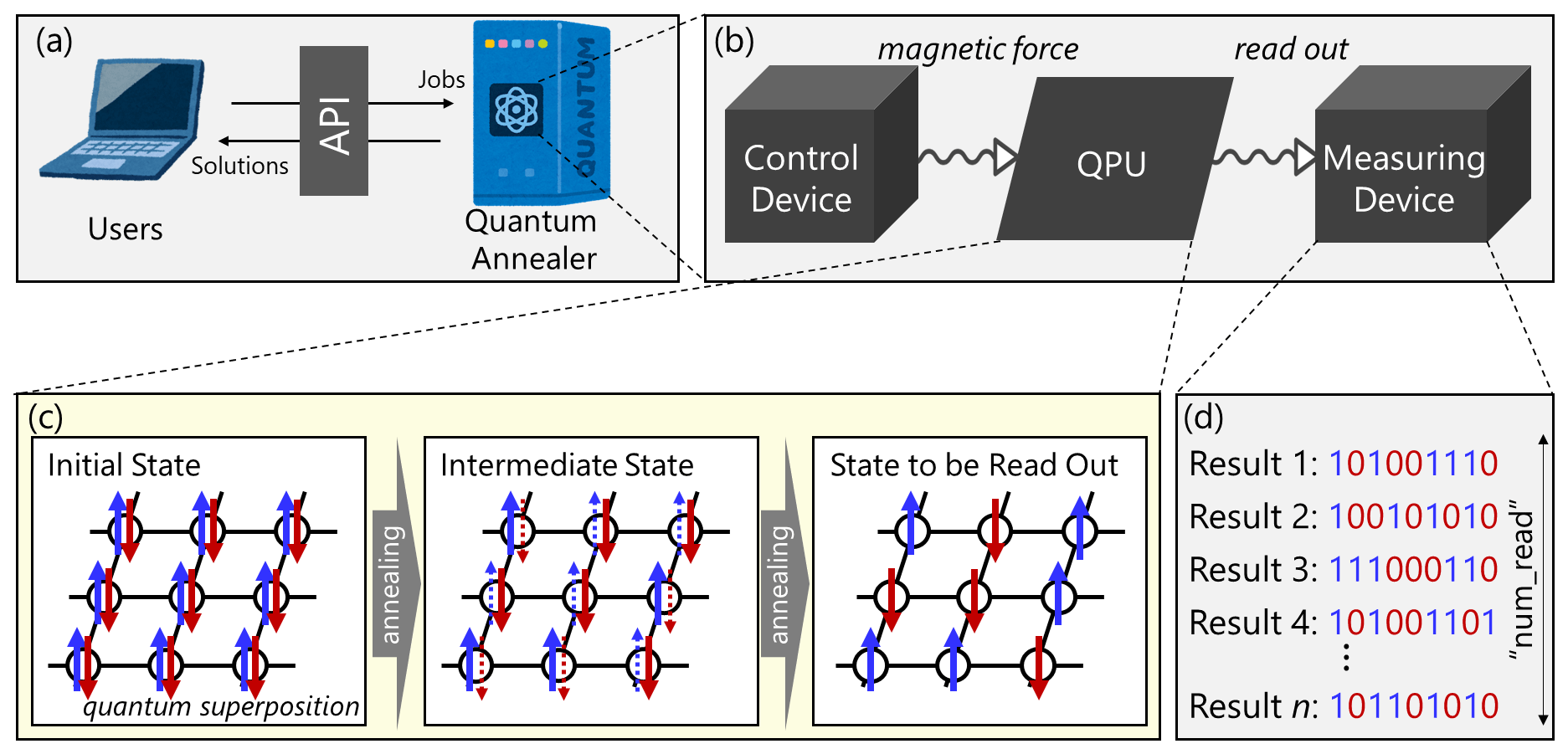
Figure A1 A conceptual image of the quantum annealing, showing (a) how users submit jobs to quantum annealers through an application programming interface (API), (b) a schematic image of the control device, quantum processing unit (QPU), and measuring device in the D-Wave quantum annealers, and (c) a schematic image of quantum annealing from an initial state with quantum superposition to a final state to be read out. Blue and red arrows in (c) represent the upward and downward spins of qubits, respectively. (d) A schematic image of states that are read out by the measuring device. Here, num_read indicates the number of times the quantum annealing process is executed and the resulting states are read out. Finally, the best result, which yielded the smallest Hamiltonian among the num_reads results, is returned to users.

This Appendix describes how quantum annealers reach the solutions of the QUBO problems. First of all, it should be noted that there are two kinds of quantum computers at this moment: quantum annealing machines and quantum gate machines. Quantum gate machines are general-purpose quantum devices capable of performing a wide range of quantum computations. The quantum gate machines enable users to design quantum circuits which manipulate qubits through gate operations to solve complex problems efficiently.

Quantum annealers are devices specialized for solving optimization problems written by the QUBO problem or Ising model. Here, a problem written by the Ising model can be reformulated to a mathematically equivalent QUBO problem and vice versa. Figure A1 provides a conceptual image of quantum annealing. Users can submit jobs (i.e., problems written by the QUBO or Ising model) to quantum annealers through an application programming interface (API) (Fig. A1a). This study used the Fixstars Amplify software development kit (known as Amplify SDK) as an API to submit jobs to D-Wave's physical quantum annealer and the Fixstars Amplify simulated quantum annealer. Figure A1b shows the functions of the control device, quantum processing unit (QPU), and measuring device, respectively. The control device regulates magnetic fields to tune the Hamiltonian of the quantum system, guiding to a low-energy state which corresponds to an optimal solution of QUBO. In QPU, quantum effects (superposition and entanglement) are leveraged to explore potential solutions of the QUBO problem through quantum annealing (Fig. A1c). The measuring device reads the final state of the QPU. Here, num_reads defines the number of states to be read from the QPU by the measuring device. Finally, a user can obtain a solution (binary vector b in this study) that yielded the smallest Hamiltonian among the num_reads states read by the measuring device.