Scaling and intermittent properties of oceanic and atmospheric pCO₂ time series and their difference in a turbulence framework

In this study, the multiscale dynamics of 38 oceanic and atmospheric pCO₂ time series from fixed Eulerian buoys recorded with 3 h resolution are considered, and their multifractal properties are demonstrated. The difference between these time series, the sea surface temperature data and the sea surface salinity data were also studied. These series possess multiscale turbulent-like fluctuations and display scaling properties from 3 h to the annual scale. Scaling exponents are estimated through Fourier analysis, and their average quantities were considered globally for all parameters, as well as for different ecosystems such as coastal shelf, coral reefs and open ocean. Sea surface temperature is the only parameter for which a spectral slope close to $\mathrm{5}/\mathrm{3}$ is found, corresponding to a passive scalar in homogeneous and isotropic turbulence. The other parameters had smaller spectral slopes, from 1.22 to 1.45. By using empirical mode decomposition of the time series, together with generalized Hilbert spectral analysis, the intermittency of the time series was considered in the multifractal framework. Concave moment functions were estimated, and Hurst indices H and intermittency parameters μ were determined in the framework of a lognormal multifractal fit. We obtained mean values of H=0.26 and 0.21, respectively, for oceanic and atmospheric pCO₂ time series and μ=0.08 for both. It is the first time that atmospheric and oceanic pCO₂ and their difference ΔpCO₂ are studied using such an intermittent turbulence framework. The ΔpCO₂ time series was shown to possess a power-law scaling with an exponent of $\mathit{\beta }=\mathrm{1.36}\pm \mathrm{0.19}$.

1 Introduction: turbulent CO₂ fluxes at the air–sea interface

Anthropogenic global carbon dioxide (CO₂) emissions have been rising since the last century (Pathak et al., 2022; Liu et al., 2022), increasing from around 4.6±0.7 GtC yr⁻¹ in the 1960s to around 11.1±0.9 GtC yr⁻¹ in recent years (Friedlingstein et al., 2023), and are linked with climate change (Anderson et al., 2016; Alola and Kirikkaleli, 2021). These emissions are partially counterbalanced by different mechanisms at different scales, from climate to small-scale turbulence. This is especially true in the oceans (Sabine et al., 2004), which absorb around 25 % of annual anthropogenic emissions (Friedlingstein et al., 2023). It is known that several other mechanisms influence the CO₂ dynamics in the ocean and the atmosphere at different spatial and temporal scales. For example, terrestrial biology (Keenan et al., 2012; Crisp et al., 2022), land chemistry (Roland et al., 2013), volcanism and human activities (Yue and Gao, 2018) can lead to variations in atmospheric CO₂. Furthermore, the ocean plays a major role in the carbon cycle through its interactions with the atmosphere and can absorb or release CO₂ via physical and biological pumps (De La Rocha and Passow, 2014; Yamamoto et al., 2018). These pumps are composed of numerous oceanic processes which also enable carbon sequestration at different timescales in the water column, e.g., through phytoplankton blooms and the thermohaline circulation (Falkowski et al., 2000; De La Rocha and Passow, 2014) and in the sediment (Henson et al., 2019).

Globally, at large temporal (e.g., annual) and spatial (e.g., planetary) scales, the ocean is a sink of CO₂. However, locally in time and space, the ocean may be a sink or a source of CO₂. In order to understand this better, in situ observations are necessary. Here we consider high-frequency fixed-point data for different parts of the global ocean, and we focus on the influence of multiscale turbulence on their fluxes. The air–sea CO₂ flux is usually written as (Wanninkhof, 2014)

$$\begin{array}{}\text{(1)}& F_{{\mathrm{CO}}_{\mathrm{2}}}=k\left(U\right)\cdot K_{\mathrm{0}}\cdot \mathrm{\Delta }p{\mathrm{CO}}_{\mathrm{2}},\end{array}$$

where K₀ is the solubility (mol L⁻¹ atm⁻¹), k(U) is the gas transfer velocity (cm h⁻¹) that depends on the surface wind speed U, and $\mathrm{\Delta }p{\mathrm{CO}}_{\mathrm{2}}=p{\mathrm{CO}}_{\mathrm{2}\mathrm{sw}}-p{\mathrm{CO}}_{\mathrm{2}\mathrm{air}}$ is the difference between partial pressures of CO₂ in equilibrium with surface water and in the air above the seawater. Turbulence has a direct influence on the different components of this formula: K₀ depends on temperature and salinity, which are turbulent scalars; k depends on wind turbulence on the atmospheric surface; and ΔpCO₂ depends on two scalars both advected by turbulence. Since k and K₀ are both positive parameters, the direction of the flux is determined by the difference ΔpCO₂: when ΔpCO₂>0, the flux goes from the sea to the atmosphere, and when ΔpCO₂<0, the ocean is locally a sink of CO₂. In this work, we focus on the scaling properties of atmospheric and oceanic CO₂ partial pressures and on their difference, using a database of Eulerian time series recorded at a time resolution of 3 h. This is considered a high-frequency measurement compared to lower-frequency measurements done from, for example, weekly or monthly sampling. In oceanography, previous work from Eulerian temperature sampling (Derot et al., 2016) on pH and carbonate dynamics (Schmitt et al., 2008; Zongo and Schmitt, 2011), as well as studies on atmospheric turbulence in the boundary layer (Schmitt et al., 1994; Katul et al., 1995; Schmitt, 2007; Calif and Schmitt, 2012, 2014), has shown that turbulent fluctuations at fixed points can be detected from hourly scales to a large scale of about 3 months. This means that, in agreement with the Richardson cascade theory (Richardson, 1922), there is an inertial range where the turbulence influence is present over a rather large range of scales from the largest (e.g., months) to the smallest (e.g., seconds). The present dataset is therefore analyzed here using methods from the field of turbulence in order to consider pCO₂ scaling properties.

The database chosen in this work is presented in Sect. 2. Then the power spectral exponents are given, and their averaged values are discussed in Sect. 3. Section 4 presents the intermittency analysis, and the discussion and conclusion of this work are in Sect. 5.

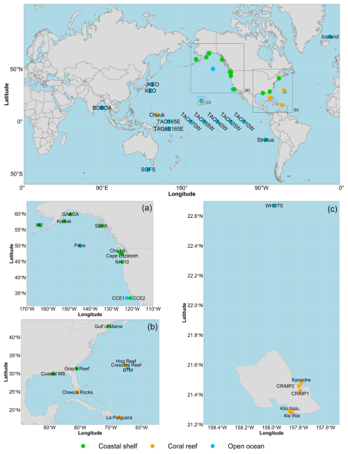
Figure 1 Maps of the positions of 38 fixed-position observation time series adapted from Sutton et al. (2018) with the same classification corresponding to a color code for coastal shelf buoys, coral reefs and open ocean ecosystems. Publisher's remark: please note that the above figure contains disputed territories.

Figure 2 Portions of time series from the BOBOA (Bay of Bengal, Indian Ocean), Cheeca Rocks (Caribbean, North Atlantic Ocean) and Gulf of Maine (North Atlantic Ocean) buoys: (a) the sea surface temperature and salinity, (b) the atmospheric and oceanic pCO₂, and (c) their difference ΔpCO₂.

2 Presentation of the database

In this work, a published in situ observational database provided by Sutton et al. (2018, 2019) is analyzed. It contains observations from 40 fixed-point autonomous buoys distributed in the Pacific, Indian, Southern and Atlantic oceans. Two sites were discarded due to different sampling frequencies, and we have considered 38 time series, whose locations are illustrated in Fig. 1 and are listed in Appendix A. For each buoy, the following parameters are recorded every 3 h: sea surface temperature (SST), sea surface salinity (SSS), seawater partial pressure of CO₂ (pCO_2 sw) and atmospheric partial pressure of CO₂ (pCO_2 air). SST and SSS are measured using a multiparameter sonde (Sea-Bird Electronics 16plus V2 SeaCAT or a SBE-37 MicroCAT, depending on the site) in the upper layer at a depth of about 0.5 m. The pCO₂ time series are calculated from the molar fraction xCO₂ by the MAPCO₂ sensor, which is an optical sensor measuring the infrared absorption by the air in comparison with the infrared absorption of a reference gas. Atmospheric measurements are done between 0.5 and 1 m from the sea surface (Sutton et al., 2014, 2019).

These buoys are classified by Sutton et al. (2019) into three categories based on the type of ecosystem in which the buoy is located. In the present work, different properties according to these ecosystems are considered. Among the 38 series, there are 11 series belonging to the coastal shelf, 10 series belonging to coral reefs and 17 series belonging to the open ocean. Sutton et al. (2019) have highlighted the appearance of anthropogenic trends and seasonality. The database has also been used in other studies: Torres et al. (2021) were interested in the mean and extreme diurnal variability of these series and have highlighted their spatial and temporal properties. These data were also used for pCO₂ data modeling purposes (Chau et al., 2022; Kwiatkowski et al., 2023).

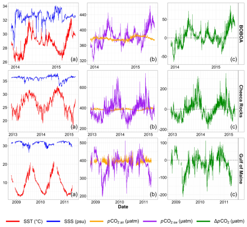
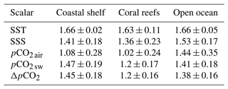
As an example, data from three sites, one from each ecosystem type, are shown in Fig. 2. They correspond to the BOBOA (Bay of Bengal, open ocean), Cheeca Rocks (Gulf of Mexico, coral reefs) and Gulf of Maine (North Atlantic Ocean, coastal shelf) time series and illustrate the multiscale variability of all the studied parameters. It is also visible in this figure that for all cases the time series of pCO_2 air presents fewer relative fluctuations than pCO_2 sw. In order to consider this property for all series, the mean, the standard deviation and the variation coefficient (ratio of the standard deviation to the mean value) of atmospheric and oceanic CO₂ partial pressures are estimated for all buoys. These quantities averaged for the three buoy categories are reported in Table 1. It shows that pCO_2 air presents much fewer relative fluctuations than pCO_2 sw: the mean values are on the same order of magnitude, whereas the variation coefficients are 6 to 8 times lower. For pCO_2 air it is between 2 % and 3 %, and for pCO_2 sw it is between 13 % and 25 %. Globally, the variation coefficient for coastal shelves is larger for atmospheric series and much larger for oceanic time series. For coral reefs and open ocean ecosystems, the mean and standard deviations are similar.

This property can be explained by the better mixing of the atmosphere (Sarmiento and Gruber, 2002). Indeed, the diffusivity coefficient of CO₂ in the atmosphere (0.16 cm² s⁻¹ at 20.1 °C; Pritchard and Currie, 1982) is about 10 000 times higher than in the seawater (1.6×10⁵ cm² s⁻¹ at 20 °C; Emerson and Hamme, 2022).

Table 1 Statistical values based on all the raw pCO₂ time series available in Sutton et al. (2019). The mean and standard deviation values are given in microatmosphere units (µatm), and variation coefficients are given in percent (%).

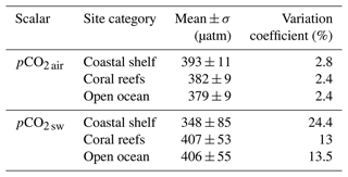
Table 2 Conditional means, standard deviations, and average proportions of positive and negative values of all the δ=ΔpCO₂ (µatm) time series averaged for each buoy site category. Conditional averages are first estimated for each time series. Then the means and standard deviations indicated in the table are estimated from these mean values.

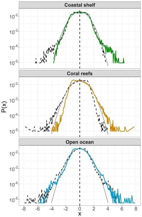
Figure 3 Probability density function (PDF) of centered time series of ΔpCO₂ considered for each site category. The dashed black lines are the symmetric PDFs, and the grey continuous lines are the Gaussian PDFs. The density has been calculated using a bandwidth of 0.05. The value represented on the x axis is the middle value of each range.

Next, the difference ΔpCO₂ is considered. First, the conditional means and standard deviations of positive and negative values are estimated, averaged over each site of each category, and shown in Table 2. The order of magnitude of the conditional mean for positive values is of the same order for the three categories, while large variations (a ratio greater than 4) are found for the conditional average of negative values. For coral reefs and open ocean ecosystems, the overall average of positive values is much larger (almost double) than the average of negative values (in amplitude). For coastal shelf ecosystems, this proportion is reversed, and the conditional average of positive values is much smaller in amplitude than the conditional average of negative values. The sink or source status of CO₂ for the different ecosystems depends on the proportion of time spent in the negative or positive values: the global mean can be written as $\langle \mathit{\delta }\rangle =p^{+}\langle \mathit{\delta }|\mathit{\delta }>\mathrm{0}\rangle +p^{-}\langle \mathit{\delta }|\mathit{\delta }<\mathrm{0}\rangle$. Table 2 indicates that when it is a sink, globally the coastal shelf ecosystems are more active sinks compared to coral reefs or open ocean ecosystems. Concerning the proportion of negative and positive values shown in the same table, it is seen that the coastal shelf sites are much more often sinks than sources (75 % versus 25 %). For the coral reef sites, it is the opposite: they are more often sources than sinks (70 % versus 30 %). In the open ocean, there is a slight proportion in favor of sinks. The probability density functions (PDFs) of ΔpCO₂ are also presented in Fig. 3 on a log scale. In these panels, the time series of ΔpCO₂ are centered (subtraction of the mean and division by the standard deviation) and then considered globally for each ecosystem (coral reefs, open ocean, coastal shelf). A Gaussian PDF is also shown for comparison. These panels show that the difference ΔpCO₂ is non-Gaussian, except for the negative values of the coastal shelf buoys. In all cases, there are more large positive values than in the Gaussian law. For open ocean buoys, the PDF is symmetric, whereas for the two other categories it is asymmetric, with more large positive values than negative ones.

3 Fourier spectral analysis

Fourier spectral analysis was applied to all series. Some portions of these time series have a time step shorter than 3 h: in order to have homogeneous time steps, these portions have been averaged to have a regular sampling of 3 h. As shown in Fig. 2, there are also large portions of missing values due to failures in measuring devices or maintenance operations. In such a case, no interpolation or averaging was performed, and the following method was used. First, the autocorrelation function was estimated, which by definition can only be considered for existing data and can deal with missing values: $C\left(\mathit{\tau }\right)=\langle X\left(t\right)X(t+\mathit{\tau })\rangle$, where X is a stationary time series with zero mean, and τ is a time increment. Then the Wiener–Khinchin theorem is used to consider the power spectrum as the Fourier transform of the autocorrelation function:

$$\begin{array}{}\text{(2)}& E\left(f\right)=\underset{-\mathrm{\infty }}{\overset{+\mathrm{\infty }}{\int }}C\left(\mathit{\tau }\right)\exp (-\mathrm{2}i\mathit{\pi }\mathit{\tau }f)\text{d}\mathit{\tau },\end{array}$$

where f is the frequency, and E(f) is the Fourier spectral density. Since the time series are considered within the framework of turbulence forcing, scaling regimes are expected with the following power-law relation (Gao et al., 2021):

$$\begin{array}{}\text{(3)}& E\left(f\right)\sim f^{-\mathit{\beta }},\end{array}$$

where “∼” means proportionality, and β>0 is the spectral slope. Let us recall that in homogeneous and isotropic turbulence the famous Kolmogorov 1941 (K41) relation corresponds to a scaling law for the velocity field with a value of $\mathit{\beta }=\mathrm{5}/\mathrm{3}$ (Kolmogorov, 1941). In such a framework, passive scalars advected by the turbulent velocity are also scaling with a scaling slope value of $\mathit{\beta }=\mathrm{5}/\mathrm{3}$ (Obukhov, 1949; Corrsin, 1951). In the ocean, temperature and salinity are generally considered to be passive scalars advected by the turbulent velocity field, whereas other scalars can also be studied, such as dissolved oxygen, concentrations of nutrients, pH, and the concentration or partial pressure of CO₂. Other values of the spectral slope have been reported and can be interpreted as the signature of a chemical or biological activity (Seuront et al., 1996; Schmitt et al., 2008; Zongo and Schmitt, 2011).

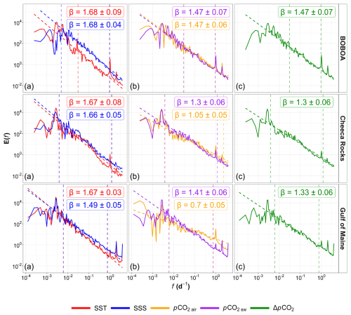
Figure 4 Fourier spectra represented in log–log format for data from BOBOA (Bay of Bengal, Indian Ocean), Cheeca Rocks (Caribbean, North Atlantic Ocean) and Gulf of Maine (North Atlantic Ocean) buoys (see Fig. 2). The dashed lines represent the power-law fits, and the slopes are given in each panel for (a) SST and SSS, (b) atmospheric and oceanic pCO₂, and (c) their difference ΔpCO₂. The dashed horizontal lines represent the range used for the estimation of the slope.

3.1 Mean values of spectral slopes

Raw Fourier spectra can be quite noisy, preventing a clear detection of scaling ranges. To prevent this, each spectrum is averaged by decade; this does not destroy spectral peaks but suppresses random fluctuations and provides smoother spectra. Over scaling ranges detected visually, the precise value of the spectral slope is estimated by using a least-squares linear fit applied to the logarithmic values. To illustrate the scaling power spectra, the Fourier spectral plots are displayed for the three time series in Fig. 4, chosen as representative of each ecosystem: BOBOA (Bay of Bengal, open ocean), Cheeca Rocks (Gulf of Mexico, coral reefs) and Gulf of Maine (North Atlantic Ocean, coastal shelf). In most cases, the scaling is found from the smallest scale (3 h to a large scale of 1 year). Peaks are found in many cases for the annual cycle, as well as for the daily and 12 h timescales, with the latter potentially corresponding to the tidal influence. The amplitude of the peaks is not the same for each series. In some cases (i.e., salinity), the scaling at high frequency is not found below the daily timescale.

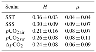
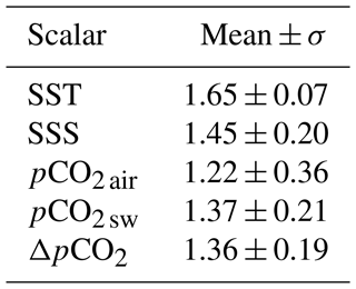
As shown in these figures, the values of the spectral slopes are variable in the range of 0.7 to 2.26, depending on the time series. This is performed for all 38 × 5 series: a spectral slope is extracted in each case, and finally the mean and standard deviations estimated over the series of both ecosystems are given in Table 3. It is found that the SST is the scalar with the lowest standard deviation in spectral slopes. The averaged SST spectral slope is also close to the value of $\mathrm{5}/\mathrm{3}$, i.e., the theoretical value expected in the case of homogeneous and isotropic turbulence. Only in a few cases are the SST spectral slopes much smaller than $\mathrm{5}/\mathrm{3}$: TAO8S165E and Kaneohe. The mean spectral slopes for the other scalars are less than $\mathrm{5}/\mathrm{3}$. The mean values for SSS, seawater pCO₂ and ΔpCO₂ are close to each other. For atmospheric pCO₂, the averaged spectral slope is the lowest. These differences in spectral slopes could be due to biological or chemical activity.

Table 3 Means and standard deviations of spectral slopes for all five parameters, estimated for the 38 global time series.

The scaling properties of atmospheric CO₂ have been reported in previous work. Spectral slopes close to $\mathrm{5}/\mathrm{3}$ have been found at high frequencies (typically for scales smaller than a few seconds, from 0.2 to 10 or 25 Hz) for measurements in the atmospheric boundary layer over a forest (Anderson et al., 1986), over a crop surface (Anderson and Verma, 1985), over vegetated fields (Ohtaki, 1985; Gao et al., 2020), over the ocean (Ohtaki et al., 1989) or over a littoral area (Sahlée et al., 2008). A more recent study reported measurements of atmospheric CO₂ using a tower 5 m above the ground in a continental zone. Scaling properties were found for scales of 10 s to 15 min, with a scaling slope of β=1.2 (Gao et al., 2020). This value is closer to the mean value found here for this parameter. However, the scales considered in the present study are much larger than the ones used in these studies and cannot be directly compared.

Figure 5 represents scatterplots of the spectral slope of some parameters. The first panel (Fig. 5a) shows that there is no direct link between the spectral slopes of the atmospheric and oceanic pCO₂; the central panel (Fig. 5b) demonstrates that there is a direct link between the spectral slope of the marine measurements and of the difference ΔpCO₂: this comes from the fact that, as seen above, the atmospheric measurements display much fewer relative fluctuations, so the oceanic fluctuations dominate in the difference ΔpCO₂. This dominance is reflected in the spectral slopes. The last panel (Fig. 5c) shows that the temperature values are very close to the theoretical value of $\mathrm{5}/\mathrm{3}$ obtained for homogeneous and isotropic turbulence, while SSS, which is also often assumed to be a turbulent passive scalar (Thorpe, 2005, 2007), displays scaling properties but with spectral slopes which are not compatible with a turbulent passive scalar.

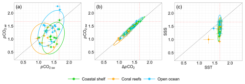
Figure 5 Scatterplots of the Fourier spectral slopes, with each dot corresponding to a given time series and its color corresponding to the ecosystem site: (a) atmospheric versus seawater pCO₂, (b) seawater pCO₂ versus the difference ΔpCO₂ and (c) SSS versus SST. The ellipses are calculated for each ecosystem from a 95 % confidence interval of the multivariate t distribution. The vertical and horizontal dashed red lines represent the value $\mathrm{5}/\mathrm{3}$. The dashed black line represents the first bisector y=x.

3.2 Analysis of spectral slopes for each ecosystem

Here statistical analysis is done over the spectral slopes of time series belonging to different ecosystems (coastal areas, coral reefs and open ocean). The different spectral slopes for all three ecosystems are represented as boxplots in Fig. 6; the mean values are also given in Table 4. Concerning SSS, the departure from the passive scalar values is smaller for open ocean sites. In coastal areas, the departures from a passive scalar slope could be due to coastal forcing induced by river flows associated with shallow depths (Crossland et al., 2005). Some sites in the equatorial Pacific (coral reef ecosystem) have slopes very different from $\mathrm{5}/\mathrm{3}$, which could be due to the associated rainfall in these areas (Turk et al., 2010). For pCO_2 air, the values for coral reefs and coastal shelf ecosystems seem similar, while for the open ocean steeper slopes are found. As mentioned above for global values, for each ecosystem the spectral slopes for the difference ΔpCO₂ are very similar to those for pCO_2 sw. Regarding the latter, it is visible that the spectral slopes are less steep for coral reef sites: such a strong departure from a passive scalar could be the effect of strong biological activity in coral reefs. The ellipses shown in Fig. 5 are calculated for each ecosystem from a 95 % confidence interval of the multivariate t distribution. They do not differentiate the ecosystems in Figs. 5.

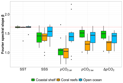
Figure 6 Representation using boxplots of all Fourier spectral slopes according to the site ecosystem (coastal shelf, coral reefs and open ocean). The dashed horizontal line corresponds to the theoretical value of $\mathrm{5}/\mathrm{3}$ that is expected for passive scalars in homogeneous and isotropic turbulence. The dots signify outliers, indicating values that fall below or above the first or third quartile (respectively) by more than 1.5 times the interquartile range (distance between the first and third quartiles).

Table 4 Means and standard deviations based on extracted Fourier spectral slopes β for each studied scalar and for each ecosystem.

3.3 Latitudinal variability of pCO₂ spectral slopes

The spatial variation of the spectral exponents of pCO₂ is considered in this section, for all series, regardless of the ecosystem to which they belong. Different bins of unequal length are chosen to perform averages, with approximately the same number of series in each bin. The result is shown in Fig. 7 where the limits of the bins are shown as dashed lines, and the mean values for atmospheric and oceanic partial pressures in CO₂ are displayed. The pattern is similar for both curves, with a minimal slope for tropical values (latitudes around 20–30°) in the Northern Hemisphere and an increase of the spectral slope as one moves away from this position. This latitudinal gradient can also be explained by the fact that there are more series belonging to the coral reef ecosystem in the database for latitudes between 20 and 30° N.

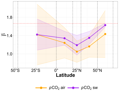
Figure 7 Average Fourier spectral slope $\stackrel{\mathrm{‾}}{\mathit{\beta }}$ as a function of latitude. The dashed red line represents the value $\mathrm{5}/\mathrm{3}$. The ranges of values used for each point are represented by the dashed black lines: [46.8° S, 0°) (3 stations), [0°, 20° N) (9 stations), [20° N, 30° N) (7 stations), [30° N, 50° N) (13 stations) and [50° N, 69° N) (6 stations).

4 Multifractal intermittency

4.1 Extraction of intermittency exponents for a time series with periodicities

Turbulent time series are intermittent and possess large fluctuations on many different scales. Such fluctuations are classically studied by considering structure functions of the form $\mathrm{\Delta }{X}_{\mathit{\tau }}=X(t+\mathit{\tau })-X\left(t\right)$, corresponding to time increments at scale τ. The scaling intermittent properties are considered by estimating the moments of order q of the structure functions (Frisch, 1995; Schmitt and Huang, 2016):

$$\begin{array}{}\text{(4)}& 〈\mathrm{|}\mathrm{\Delta }{X}_{\mathit{\tau }}{\mathrm{|}}^q〉\sim {\mathit{\tau }}^{\mathit{\zeta }\left(q\right)},\end{array}$$

where q>0 is the moment order (which can be non-integer), and ζ(q) is the scaling exponent of the corresponding moment function. Larger moments correspond to more-intense fluctuations, and the whole ζ(q) curve characterizes the multiscale intermittency of the time series. The Fourier spectrum corresponds to a moment of order 2, and the spectral exponent β is related with ζ(2): $\mathit{\beta }=\mathrm{1}+\mathit{\zeta }\left(\mathrm{2}\right)$.

Unfortunately, the periodicity in the series, even if weak, is known to destroy the scaling properties of structure functions (Huang et al., 2011; Schmitt and Huang, 2016), and in this case other methods are needed to extract the scaling exponent ζ(q). This is done here in the spectral space by using the Hilbert spectral analysis (HSA) associated with empirical mode decomposition (EMD-HSA), using the generalized HSA method. This method first uses the EMD, which is an algorithm developed to decompose the original time series into N other time series called intrinsic mode functions (IMFs; Huang et al., 1998, 1999; Flandrin et al., 2004). This signal analysis has already been used to study multiscale variability of CO₂ time series (Landschützer et al., 2016; Zhang et al., 2022). The sum of IMFs C_i(t) and a residue r_n(t) gives the original signal X(t):

$$\begin{array}{}\text{(5)}& X\left(t\right)=\sum _{i=\mathrm{1}}^N{C}_i\left(t\right)+r_n\left(t\right).\end{array}$$

This iterative algorithm is based on a spline interpolation of local minima and maxima. Each IMF is a zero-mean time series localized in the frequency space. Their Hilbert transform is denoted ${\stackrel{\mathrm{̃}}{C}}_i\left(t\right)$:

$$\begin{array}{}\text{(6)}& {\stackrel{\mathrm{̃}}{C}}_i\left(t\right)={\displaystyle \frac{\mathrm{1}}{\mathit{\pi }}}\mathrm{PV}\underset{-\mathrm{\infty }}{\overset{+\mathrm{\infty }}{\int }}{\displaystyle \frac{C_i\left(\mathit{\tau }\right)}{t-\mathit{\tau }}}\text{d}\mathit{\tau },\end{array}$$

where PV indicates the Cauchy principal value. The analytic signal $z_i=C_i+j{\stackrel{\mathrm{̃}}{C}}_i$ is a complex number that can be written as $z_i=A_i\left(t\right)e^{j{\mathit{\theta }}_i\left(t\right)}$, where A_i(t) is the local amplitude and θ_i(t) the local phase of C_i(t). Leaving the residual, the original signal can be rewritten as the sum of the real part of all the analytic signals z_i as $X\left(t\right)=Re{\sum }_{i=\mathrm{1}}^N{A}_i\left(t\right)e^{j{\mathit{\theta }}_i\left(t\right)}$. This transformation needs regular time steps as is done when using the fast Fourier transform (Huang and Schmitt, 2014). The missing data were so replaced by the value 0. Here, a local instantaneous frequency is extracted from ω = d$\mathit{\theta }/$dt (where the phase θ(t) is given by ${\mathit{\theta }}_i\left(t\right)={\tan }^{-\mathrm{1}}{\stackrel{\mathrm{̃}}{C}}_i\left(t\right)/C_i\left(t\right)$). When we have the instantaneous frequency information, missing data parts are then excluded in the following steps. A joint probability density function of frequency and amplitude p(ω,A) is extracted from the data, and a Hilbert power spectrum is computed as $L_{\mathrm{2}}\left(\mathit{\omega }\right)={\int }_{\mathrm{0}}^{+\mathrm{\infty }}p(\mathit{\omega },A)A^{\mathrm{2}}\text{d}A$. This Hilbert spectrum is similar to the Fourier spectrum E(f) (Huang et al., 2008). To consider the intermittency of the signal in the EMD-HSA framework, the Hilbert marginal spectrum L_q(ω) is calculated for different statistical moments q (Huang et al., 2008, 2011; Schmitt and Huang, 2016) as $L_q\left(\mathit{\omega }\right)={\int }_{\mathrm{0}}^{+\mathrm{\infty }}p(\mathit{\omega },A)A^q\text{d}A$. For scaling time series, it has been shown that this can be written as

$$\begin{array}{}\text{(7)}& L_q\left(\mathit{\omega }\right)\sim {\mathit{\omega }}^{-\mathit{\xi }\left(q\right)}\end{array}$$

for frequencies belonging to the scaling range, where the scaling exponent in the amplitude–frequency space ξ(q) is related to the structure function scaling exponents (also called scaling moment function) as $\mathit{\zeta }\left(q\right)=\mathit{\xi }\left(q\right)-\mathrm{1}$. It was previously shown using simulations that this EMD-HSA approach, with the estimation of multifractal exponents in the frequency space, is not affected by the periodicity in the original series (Huang et al., 2011).

This method is applied here to the time series to extract intermittency exponents. There are several intermittency models published in the literature (Schmitt and Huang, 2016). The classical one is the lognormal model originally proposed by Kolmogorov (Kolmogorov, 1962). This model provides a quadratic expression which is chosen here as a fit of the nonlinear curve of the ζ(q) function. In this framework, the scaling exponent can be written as $\mathit{\zeta }\left(q\right)=qH-K\left(q\right)$, where H=ζ(1) is the Hurst exponent (usually $\mathrm{0}\le H\le \mathrm{1}$) and K(q) captures the intermittency corrections. In the lognormal framework, only one more parameter is needed here, the intermittency parameters $\mathit{\mu }=K\left(\mathrm{2}\right)=\mathrm{2}H-\mathit{\zeta }\left(\mathrm{2}\right)$. These two parameters are extracted from the EMD-HSA exponents ξ(q).

4.2 Intermittency analysis of the database

The EMD-HSA method has only been applied here to 28 stations among the 38 studied stations: for the remaining 10 stations (8 coral reefs and 2 open ocean sites), the scaling of moments of order larger than 2 was destroyed due to too low a number of data points in the series. The results for the three specific stations chosen as representative of the three ecosystems are shown in Fig. 8 for moments from 0 to 4. The shape of scaling exponent ζ(q) is concave as expected. Some scaling exponents are almost linear, which means that the intermittency correction is weak. The overall nonlinear and concave shapes are captured by the two parameters H and μ. The larger μ is, the more important the intermittency corrections are. These parameters are estimated for each series, and their mean and standard deviation are provided in Table 5. The values of H are estimated from the first-order moment using the EMD-HSA method, whereas the values of the spectral slopes β are estimated using Fourier analysis: this means that there may be some slight differences due to the method and intermittency corrections, but globally the relation $\mathit{\beta }\simeq \mathrm{1}+\mathrm{2}H$ is approximately valid.

Concerning the intermittency parameter, let us note that if the same procedure is applied to the velocity and passive scalar in fully developed hydrodynamic turbulence (H=ζ(1) and $\mathit{\mu }=\mathrm{2}\mathit{\zeta }\left(\mathrm{1}\right)-\mathit{\zeta }\left(\mathrm{2}\right)$), we obtain values of H=0.37 and μ=0.04 for the velocity field (Schmitt, 2006) and H=0.38 and μ=0.12 for the passive scalar field (Schmitt et al., 1996). The values found here for μ are on the same order of magnitude and sometimes slightly smaller than what is found for the passive scalar in hydrodynamic turbulence. The results obtained also show that, overall, the intermittency parameter is greater for the salinity and partial pressure of CO₂ time series. It also shows for the first time the multifractal intermittency of oceanic and atmospheric pCO₂ fields.

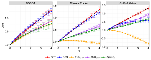
Figure 8 The scaling moment function $\mathit{\zeta }\left(q\right)=\mathit{\xi }\left(q\right)-\mathrm{1}$ of the BOBOA, Cheeca Rocks and Gulf of Maine buoy time series for different statistical moments q from 0 to 4. The dashed line represents the theoretical relation $q/\mathrm{3}$ that is linked to monofractal dynamics with $H=\mathrm{1}/\mathrm{3}$ as in homogeneous and isotropic turbulence with no intermittency.

Table 5 For all five parameters, the Hurst index H and the intermittency parameter μ are shown with means and standard deviations estimated for the 28 time series. For homogeneous and isotropic turbulence, the expected value for H is $\mathrm{1}/\mathrm{3}$ with an experimental intermittency parameter μ≃0.04.

5 Discussion and conclusion

Here, a database of high-frequency fixed-point buoys recording at 3 h resolution has been considered. The dynamics of sea surface temperature, sea surface salinity, seawater and atmospheric partial pressures of CO₂ and the difference ΔpCO₂ have been considered for each site. These quantities are scalars forced and transported by turbulence; they display large turbulence-like fluctuations at many different scales, and their multiscale dynamics have been considered by using the Fourier transform: it was found that these series have scaling properties from the smallest scale (3 h) to 1 year. Mean spectral slopes have been estimated: the SST possessed spectral slopes on average close to the value of $\mathrm{5}/\mathrm{3}$, corresponding to 3D passive scalars in homogeneous and isotropic turbulence. The other scalars displayed values of the spectral slope β that are much smaller, from about 1.22 to 1.45, indicating a behavior different from a purely passive scalar of turbulence. Such values have already been found for other scalars (fluorescence, pH) in marine waters for the same range of scales (Seuront et al., 1996; Schmitt et al., 2008; Zongo and Schmitt, 2011). Mean values were also estimated on average for different ecosystems (coastal shelf, coral reefs and the open ocean), and some differences could be detected. There were also latitudinal variations in these slopes.

The Kolmogorov–Obukhov–Corrsin slope of $\mathrm{5}/\mathrm{3}$ for passive scalars was obtained through dimensional analysis. Let us emphasize here that similar theoretical explanations for slopes close to $\mathrm{6}/\mathrm{5}$, $\mathrm{4}/\mathrm{3}$ or $\mathrm{5}/\mathrm{2}$ for the scalars considered are not presently available; in future studies, dimensional analysis could be explored in this framework.

Power spectra correspond to second-order moments and medium fluctuations. To study the intermittent and multifractal properties of the series, the EMD-HSA method was used, since the classical structure function approach cannot be used for series possessing periodicity as is the case here, with daily and tidal forcing. This approach could not be used for all series since it needs rather large datasets. It was used for 28 series, and the multifractal properties were characterized by considering a lognormal fit, with the estimation of the Hurst exponent H and the intermittency parameter μ. This showed that, in general, the different time series possess multifractal properties with various intensities of the intermittency exponent (the largest being found in SSS and pCO₂). We may note also that the approach used here is consistent with previous studies involving singular spectral analysis and assumptions of multifractality for oceanic pCO₂ data (Hernández-Carrasco et al., 2015, 2018).

Considering pCO₂ series, one of the interesting points in the present time series is the fact that simultaneous measurements of atmospheric and oceanic pCO₂ are estimated. It was found that the variation coefficient of atmospheric pCO₂ (ratio of standard deviation to the mean) is much lower than for the marine waters with a ratio of 6 to 8. Furthermore, the difference ΔpCO₂ was studied here and shown to be scaling and multifractal, and, to the best of our knowledge, it is the first time that this quantity is shown to have multifractal properties. In the framework of the lognormal multifractal model, we have provided the two parameters H=0.24 and μ=0.06. These parameters characterize the intermittency of the CO₂ flux between air and water in the range of scales which was considered here, i.e., on average between a few days and 1 year. This is clearly related to turbulent forcing. Since the direction of the flux and the fact that a given site is a sink or a source of CO₂ are given by the difference ΔpCO₂, such turbulent forcing is an important point for future studies; these studies should (i) perform the same analysis at smaller scales using higher-resolution measurements, (ii) see more precisely how the turbulent forcing influences the sign of the difference, and (iii) see how the intermittency properties of these differences are related to the forcing and climate of a given site. The influence of the ecosystem found here for some average values of the parameter β is a first step in this direction.

Appendix A: Summary of the database

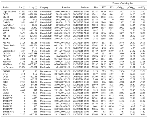
Table A1 contains information about the complete database: locations, categories, time coverage, sizes and proportions of missing data.

Table A1 Summary table of all time series in the studied database (Sutton et al., 2019). The time resolution for each of these time series is 3 h.