the Creative Commons Attribution 4.0 License.
the Creative Commons Attribution 4.0 License.
 | 10 Jan 2024
Stability and uncertainty assessment of geoelectrical resistivity model parameters: a new hybrid metaheuristic algorithm and posterior probability density function approach
Kuldeep Sarkar
Jit V. Tiwari
Upendra K. Singh
Estimating a reliable subsurface resistivity structure using conventional techniques is challenging due to the nonlinear nature of the inverse problems. The performance of the inversion techniques can be pretty ambiguous based on the optimal error, although traditional methods have proven to be quite effective. In this work, the impacts of the constraints accessible from a borehole are examined for further assessment and to enhance algorithm effectivity. The vPSOGWO strategy is a new approach that is based on a model search space without any prior information, and it describes the hybridization of particle swarm optimization (PSO) with the Grey Wolf Optimizer (GWO). To understand the efficiency and novelty of the algorithm, it has been validated on two different kinds of synthetic resistivity data with various sets of noise and, subsequently, applied to three field datasets of different geological terrains. The analyzed results suggest that the subsurface resistivity model shows considerable uncertainty. Thus, it is superior to examine the histograms and posterior probability density functions (PDFs) of such solutions to exemplify the global solution. A PDF with a 68.27 % confidence interval (CI) selects a region with a higher probability. Therefore, the inverted models are used to estimate the mean global solution and the most negligible uncertainties, where the mean global solution represents the best solution. Our vPSOGWO-inverted outcomes have been proven to be more accurate than classic PSO, GWO, and state-of-the-art variants of classic approaches. As a result, this novel method plays a vital role in vertical electrical sounding (VES) data inversion.
- Article
(3797 KB) - Full-text XML
- BibTeX
- EndNote


The vertical electrical resistivity sounding (VES) technique is an economical and simple method that has been used to determine the layered parameters in a wide range of applications in the hydrogeological, groundwater, mineral, geothermal, hydrocarbon, engineering, and environmental fields, among others (Sen et al., 1993; Sharma, 2012; Panda et al., 2018). VES data interpretation is challenging due to its unstable, nonunique solution and algorithm sensitivity (Narayan et al., 1994; Oldenburg and Li, 1994; Singh et al., 2005, 2013). Therefore, many researchers have developed several inversion algorithms to improve accuracy and stability and to reduce uncertainty in the solutions. These inversion techniques are grouped into local and global optimization techniques. In the local inversion techniques, a logical initial guess is required to get the solution. This has led researchers to think about alternative methods via which a broad range of parameters can be established. Researchers have developed various metaheuristic optimization algorithms to solve various real-world problems. These algorithm types, inspired by natural phenomenon, include ant colony optimization (ACO; Colorni et al., 1991), the Bat Algorithm (Yang, 2010), biogeographically based optimization (Simon, 2008), differential evolution (DE; Storn and Price, 1997), the Firefly Algorithm (Yang, 2010), the Genetic Algorithm (GA; Whitley, 1994; Mitchell, 1998), the Gravitational Search Algorithm (GSA; Rashedi et al., 2009), the Grey Wolf Optimizer (GWO; Mirjalili et al., 2014), and particle swarm optimization (PSO; Kennedy and Eberhart, 1995). These optimization techniques aim to have an optimum solution and fast convergent rate to obtain global minima. However, unique characteristics, namely, exploration and exploitation, in global optimization algorithms persist. For example, PSO has a very high potential regarding exploitation, implying that the algorithm performs well with respect to a local search (Şenel et al., 2019), but it is inferior regarding exploration, which means that the algorithm has less ability with respect to establishing the starting position near global minima and, due to low exploration characteristics, it gets trapped at the local minima (Eiben and Schippers, 1998; Mirjalili and Hashim, 2010). Therefore, integrating two algorithms with the opposite characteristics is the best way to solve the exploration characteristics and exploitation characteristics and to provide a more accurate and reliable solution, compared with results obtained with an individual algorithm. Many authors have developed various hybrid metaheuristic algorithms such as PSOGA for fundamental function analysis, PSOACO for data mining, PSODE for global optimization using the standard function, and PSOGSA using the standard function (Esmin et al., 2013; Lai and Zhang, 2009; Rashedi et al., 2009).
This study focuses on a variable-weight hybrid algorithm, known as vPSOGWO (Şenel et al., 2019), that fuses the exploration ability of PSO with the exploration ability of GWO. In this algorithm, some random particles of PSO are replaced with new ones obtained from GWO. In prior work, the constant-weight hybrid technique of PSO and GWO, known as HPSOGWO, has been used by some authors for different applications, such as for single-area-unit commitment problems (Kamboj, 2015), mathematical problems (Singh and Singh, 2017), and benchmark functions and real-world issues (Şenel et al., 2019). However, to the best of our knowledge, none of these researchers have tested these methods on geophysical data inversion. Thus, in this study, the applicability of the vPSOGWO algorithm is demonstrated on synthetic data with noise, synthetic data without noise, and various field resistivity sounding data to estimate the resistivity distribution in a 1D Earth's subsurface model. This work also calculates the posterior probability density functions (PDFs) with a 68.27 % confidence interval (CI) and correlation matrix on all accepted models to determine the mean global model and uncertainty. As a result, we analyzed and compared the effectiveness of the proposed algorithms with classic PSO, GWO, and state-of-the-art variants of classic methods. Our analysis advocates for the fact that the vPSOGWO algorithm produces a more accurate and reliable model with excellent stability, the least model uncertainty, and the ability to successfully resist noise.
With the help of the kernel function (Koefoed, 1979) and Schlumberger resistivity configuration (Fig. 1), the forward code is developed and synthetic resistivity datasets are produced from known parameters, such as the current electrode spacing and the number of geological multilayers of true resistivities and their corresponding thicknesses. The mathematical expression of the apparent resistivity is expressed as follows:
where J1 is the first-order Bessel function, λ represents the integration variables, s is the current electrode spacing, and m is the model.
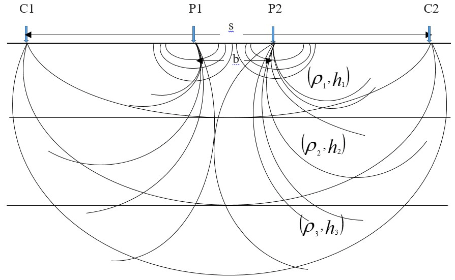
Figure 1Schlumberger array configuration for the three-layer case: C1 and C2, through which the current is injected, are current electrodes with spacing s, while P1 and P2 are potential electrodes with spacing b.
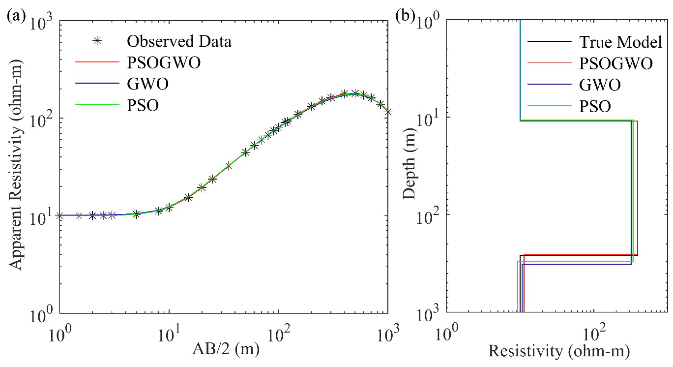
Figure 2Three-layer synthetic data: (a) observed data (*) and best-fitted calculated apparent resistivity curve (>68.27 % PDF); (b) the 1D mean model (>68.27 % PDF) for the true model (black), vPSOGWO (red), GWO (blue), and PSO (green).
For each layer, the kernel's resistivity transform Tk has been determined by Pekeris (1940). The apparent resistivity, Tk(λ), is convoluted with linear filter theory to compute the following:
The geophysical inverse problem can be formulated through a forward modeling operator/functional with the aim of achieving the geophysical model/solution that best illuminates the observed data. This operator integrates the geophysical problems and maps between the observed data y and the solution x as follows:
The inversion techniques minimize the cost functional/misfit functional, which is generally a degree of the relationship between the N number of observed data (yo) and the calculated data (yc). This misfit functional can be introduced here as a mean square error (MSE) and can be defined as follows:
3.1 Particle swarm optimization
Particle swarm optimization (PSO) is based on the social behavior of animals, such as the schooling behavior of fish or the flocking behavior of birds (Kennedy and Eberhart, 1995). When birds go in search of food, they scatter randomly within a search space before they can determine the position of food. While searching for food, there is always a bird who is aware of the position of food, and they share this information with others. Using this method, each bird is referred to as a particle and is represented by geophysical solutions/models (i.e., here, a particle is a resistivity layer parameter). The capability/fitness of each swarm/bird is estimated between the N number of observed data (yo), which measure the swarm and the food distance, and the computed data (yc), which measure the swarm and the estimated position (resistivity layer parameter/solution) of the prey distance using Eq. (4).
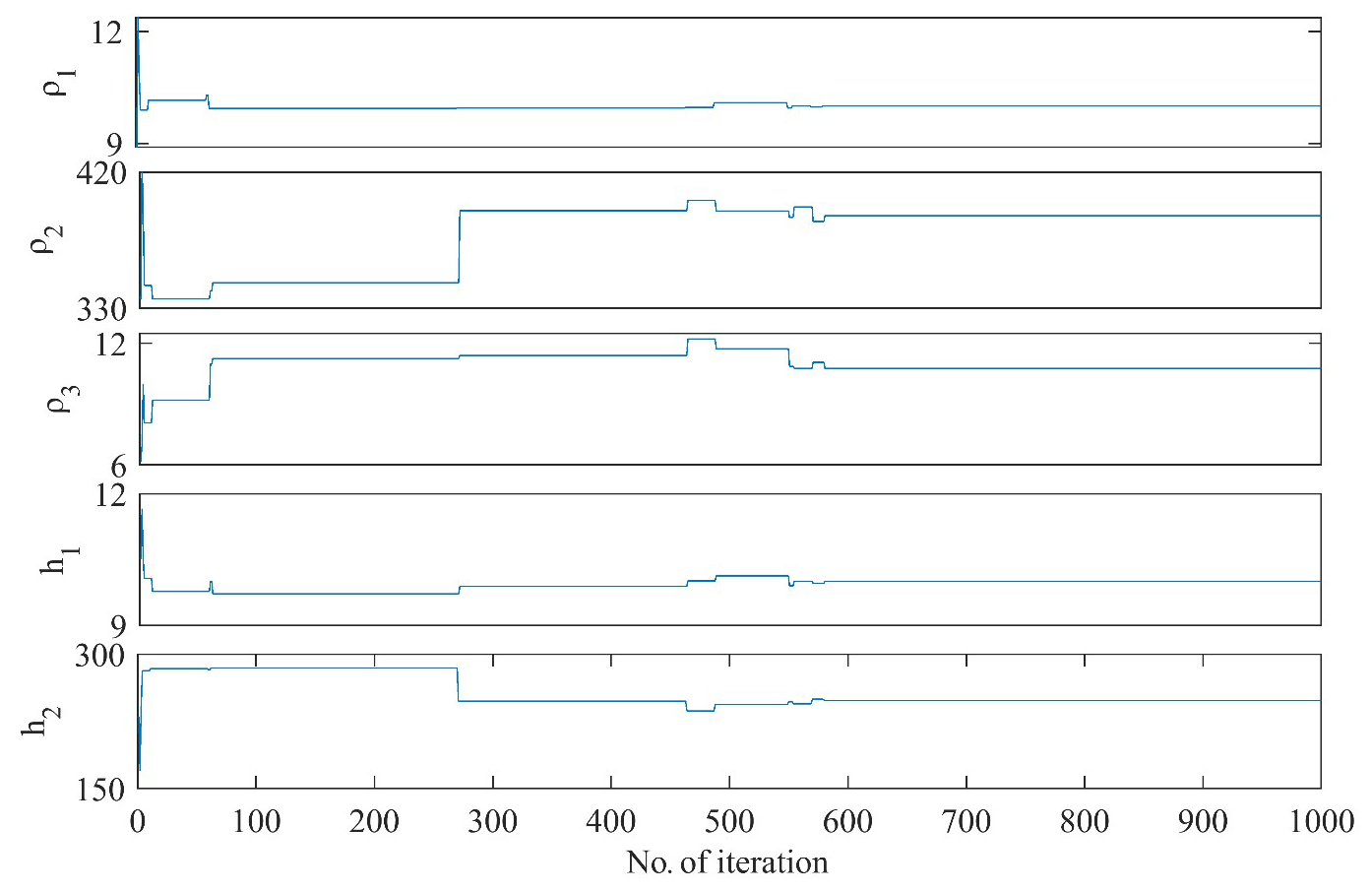
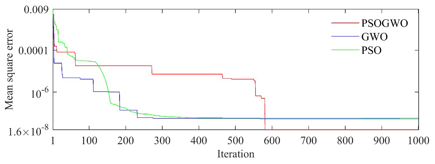
Figure 4Convergent curve, also known as the error versus iteration curve, for three-layer noiseless synthetic data.
The best position among particles with information about it is stored in memory for each iteration. The new velocity and position of the population pool are accepted if their possibility is large, otherwise they are rejected. In that case, the particles are randomly distributed in the search space in order to escape the local optima. The search continues until it gains a maximum possibility or reaches the maximum iteration. In the global search space, the position of each particle is updated by the following two mathematical equations:
Here, vi represents the velocity of the ith particle with position xi, xp is the best position obtained by the ith particle, xg is the best position, t is the number of the iteration, i represents the number of the model (, rand represent the random values with a range of [0, 1], and the coefficients c1 and c2 represent the optimization parameter. The disadvantage of the PSO algorithm is that, while directing particles to random positions, it has a small possibility of escaping the local minima.
3.2 The Grey Wolf Optimizer (GWO) algorithm
The GWO algorithm mimics the leadership hierarchy and hunting mechanics of grey wolves and is used to solve both standard and real-life problems. In the grey wolf community, animals are divided in four groups: (i) alpha animals, (ii) beta animals, (iii) delta animals, and (iv) omega animals. Alpha, beta, and delta animals are the fittest wolves, and they guide omega animals towards promising areas of the search space. The alpha is the pack leader and generally makes important and final decision for all of the wolves; thus, the alpha represents the fittest solution. The betas are subordinates and help the alphas in their decision-making. However, betas cannot force alphas into any decision; they can only order the lower wolves. The beta group takes orders from the alpha group, enforces orders with respect to the other groups, and sends feedback back to the alpha group. All of the groups are dominant with respect to the omega group. Nevertheless, the omega group is an important component of the pack during hunting, as they play the role of the scapegoat and are only allowed to eat at the end. If a wolf is not part of the alpha, beta, or omega group, they are known as delta and only summit to alpha and beta groups. In the GWO algorithm, the alpha group represents the best position, i.e., geophysical model/solution. In our case, the geophysical model is the resistivity layer parameters. The beta and delta groups are consecutive best solutions, and the omega group is the best solution that always follows the other groups. The capability/fitness of each wolf is estimated between the observed data (which measure the wolf and prey distance) and the computed data (which measure the wolf and the estimated position of the prey distance) using Eq. (4).
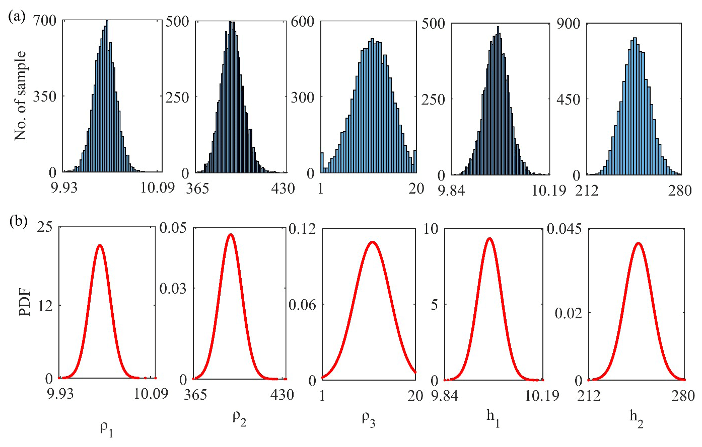
Figure 5(a) Histogram and (b) posterior PDF of all 10 000 solutions corresponding to the output of each run for the three-layer synthetic Earth model.
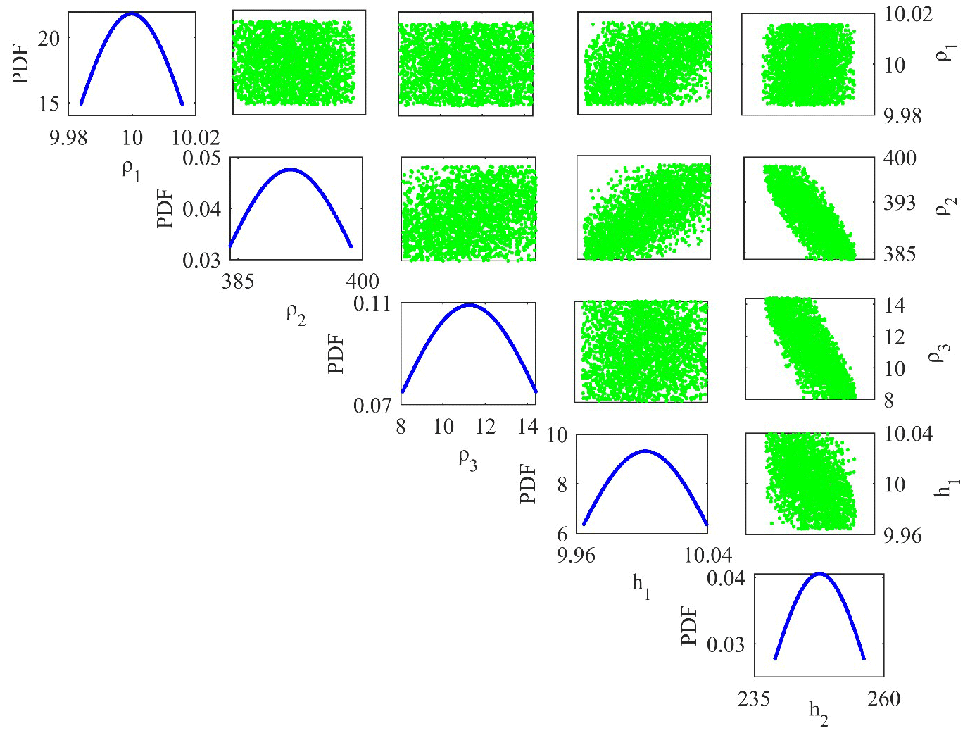
Figure 6Correlation plot between model parameters (off-diagonal) and the posterior PDF curve (diagonal) for those models whose PDF exceeds 68.27 % of the confidence interval (CI).
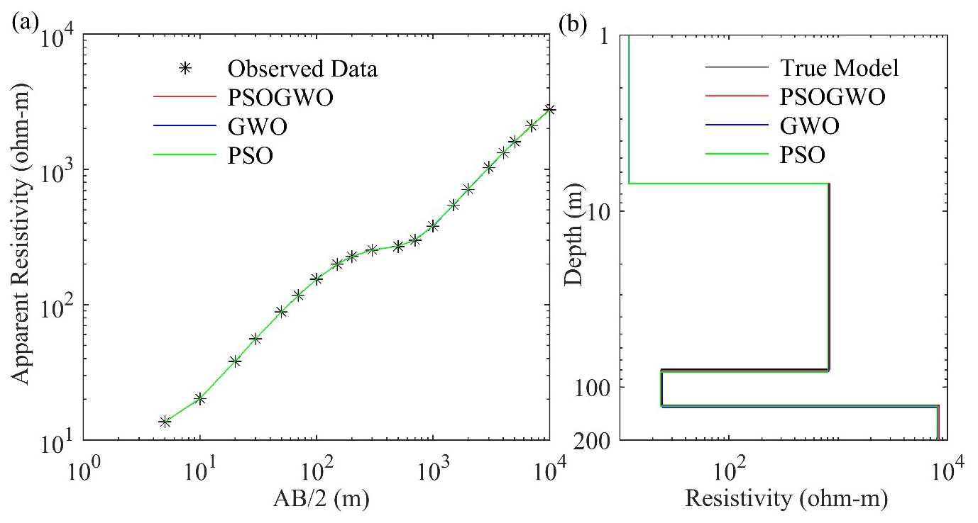
Figure 7Four-layer synthetic data: (a) observed data (*) and the best-fitted calculated apparent resistivity curve (>68.27 % PDF); (b) the 1D mean model (>68.27 % PDF) for the true model (black), vPSOGWO (red), GWO (blue), and PSO (green).
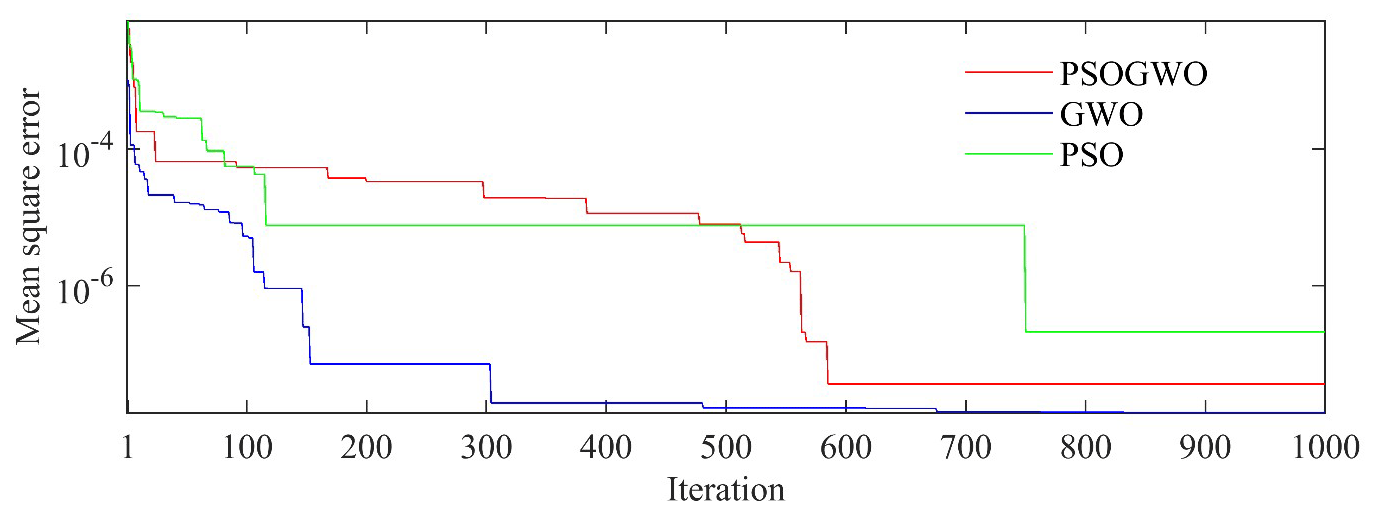
Figure 8Convergent curve, also known as the error versus iteration curve, for four-layer noiseless synthetic resistivity sounding data.
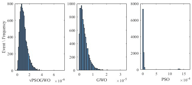
Figure 9Histogram of the logarithmic mean square error for vPSOGWO, GWO, and PSO over 10 000 models. The x axis of the three histograms represents the misfit error corresponding to 10 000 models.
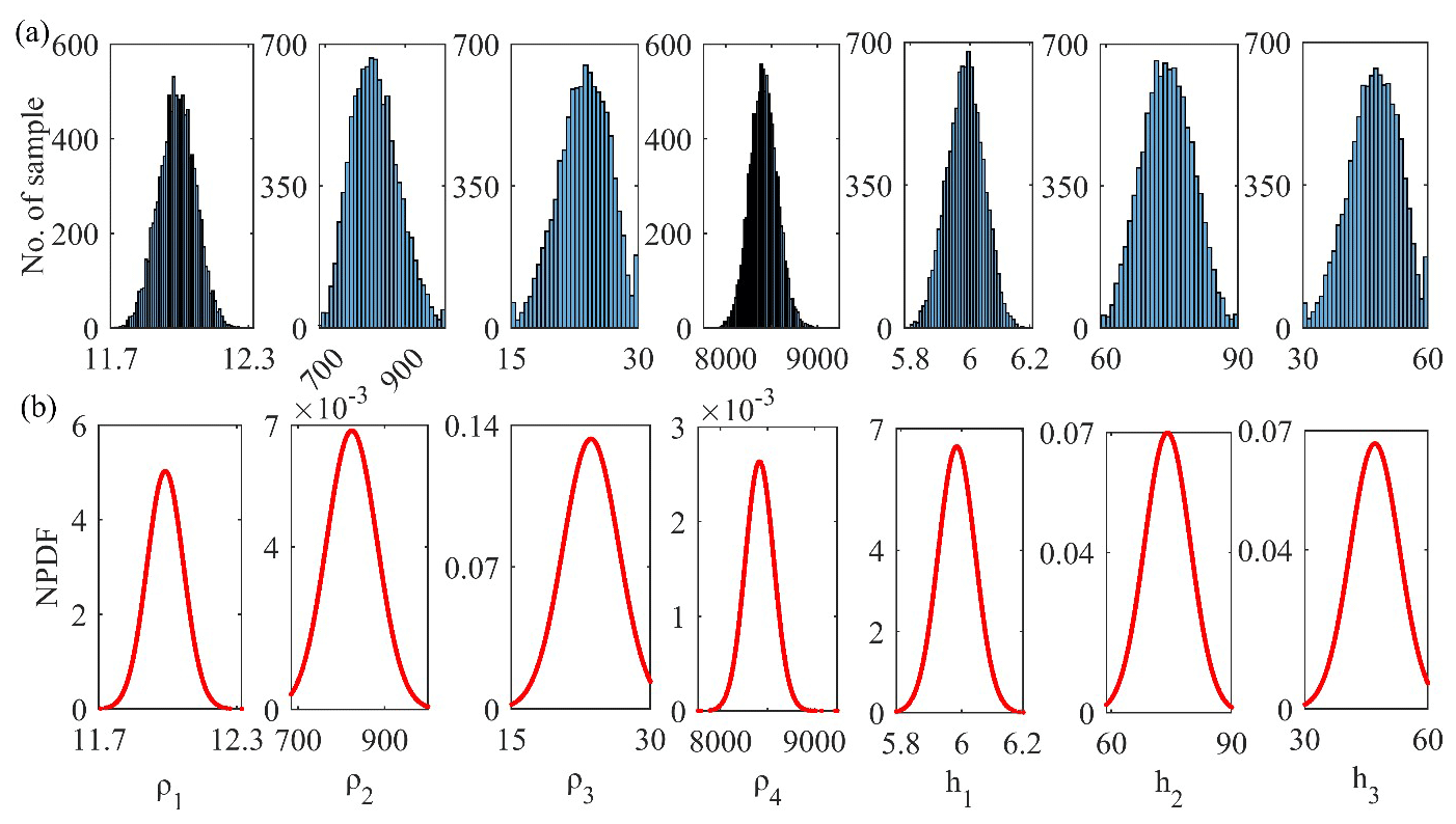
Figure 10(a) Histogram and (b) posterior PDF of all 10 000 solutions corresponding to the output of each run for four-layer synthetic resistivity sounding data.
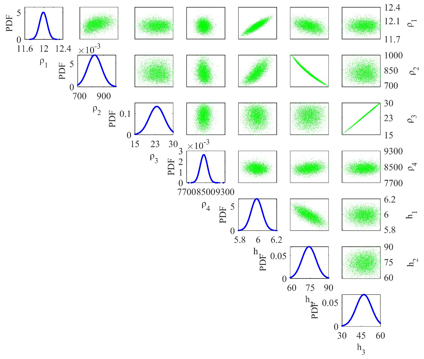
Figure 11Correlation plot between the model parameters (off-diagonal) and posterior PDF curve (diagonal) for models whose PDF exceeds 68.27 % of the confidence interval (CI).
Hunting in the grey wolf community has been divided into three groups: searching for prey, encircling the prey, and attacking the prey. The encircling nature of the wolves is defined by the following equations:
Here, xp is the prey position, xi is the grey wolves' positions, and a and c are the vectors mathematically formulated as follows:
Here, and varies from 2 to 0 in decreasing order with increasing iteration (t), l represents the maximum iteration, and rand is the random number in the range of [0, 1].
In the grey wolf community, the alpha group leads, the beta and the delta groups search for the prey location, and the omega group follows the other groups. Therefore, the alpha group gives the best solution, while the respective second- and third-best solutions are provided by the beta and the delta groups. Thus, the remaining wolves, i.e., the omega group, follow the best solution (the other wolf groups) to obtain the best location. This is mathematically equated as follows:
The best location/position for alpha, beta, and delta wolves in each iteration is given by xα, xβ, and xδ, respectively:
Here, xp(t+1) describes the updated position of the prey in the (t+1) iteration and is obtained from the mean position of three best wolves in the population; thus,
The values of a are utilized by wolves who force the search to move away from the prey. When a≥1, hunting is abandoned in order to find a better solution; in contrast, when a<1, the wolves are forced to attack the prey. In Eq. (9), a varies in the range of .
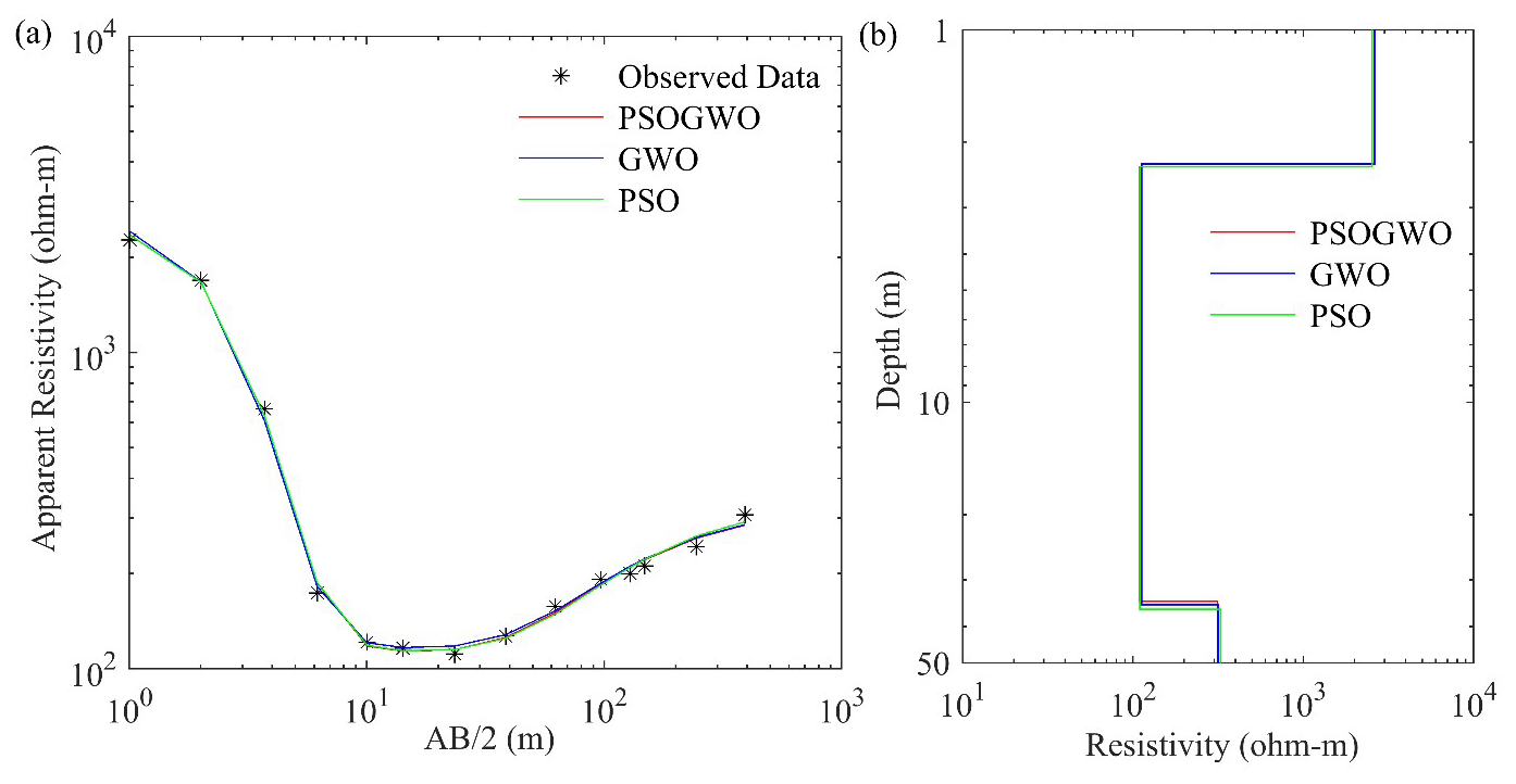
Figure 12Three-layer field data over Mount Turner, northern Queensland, Australia: (a) observed data (*) and the best-fitted calculated apparent resistivity curve (>68.27 % PDF); (b) the 1D mean model (>68.27 % PDF) for the true model (black), vPSOGWO (red), GWO (blue), and PSO (green).
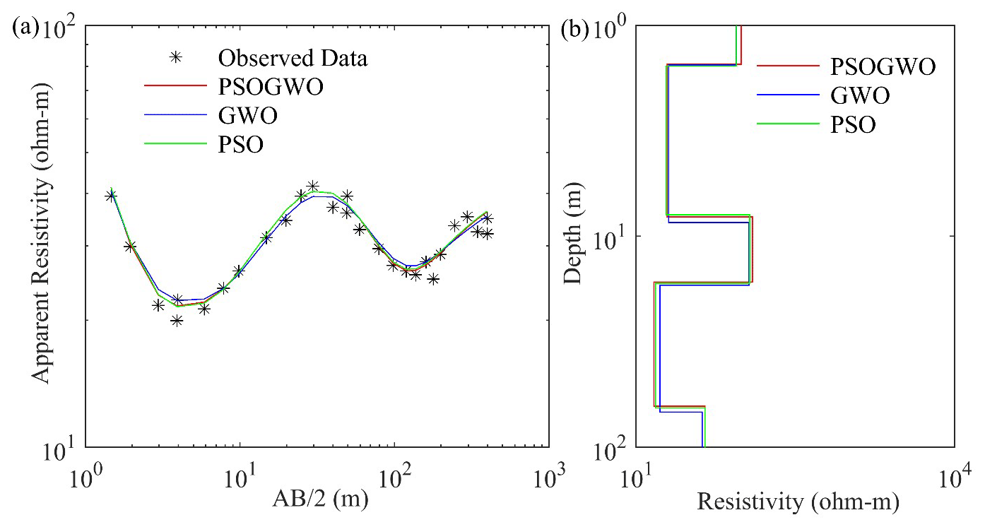
Figure 13Five-layer field data: (a) observed data (*) and the best-fitted calculated apparent resistivity curve (>68.27 % PDF); (b) the 1D mean model (>68.27 % PDF) for the true model (black), vPSOGWO (red), GWO (blue), and PSO (green).
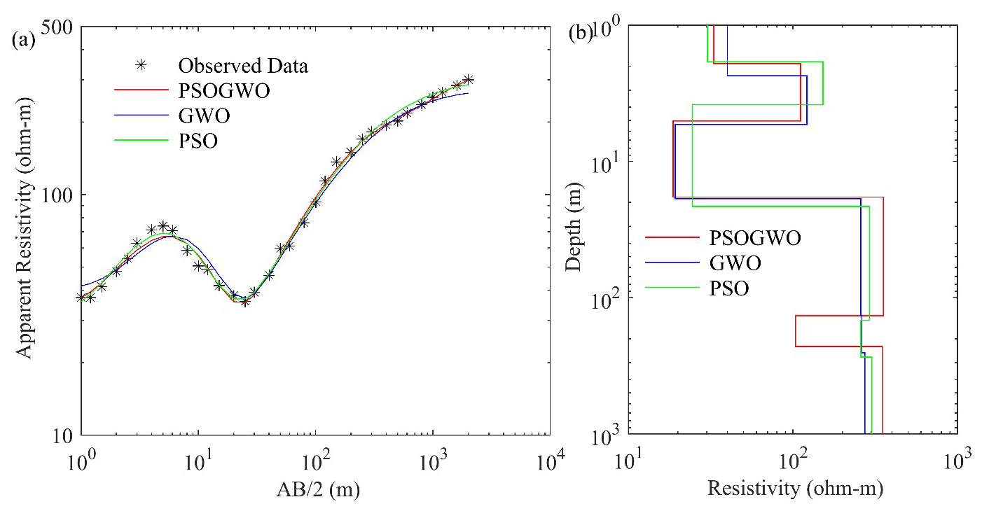
Figure 14Six-layer field data over Keshiari (Kharagpur), India: (a) observed data (*) and the best-fitted calculated apparent resistivity curve (>68.27 % PDF); (b) the 1D mean model (>68.27 % PDF) for the true model (black), vPSOGWO (red), GWO (blue), and PSO (green).
3.3 Variable-weight hybrid PSOGWO (vPSOGWO)
Despite usefulness of the PSO technique with respect to achieving successful results in real-world problems, it tends to fall into the local minima, causing the solution to move away from global minima. This tendency for deterioration within the local minima is stopped by the explorative ability of the GWO algorithm. Therefore, the variable-weight hybrid PSOGWO, known as vPSOGWO, fuses the exploitation potential of PSO with the exploration potential of GWO to overcome each other's discrepancy via the implementation of varying weight. Due to the involvement of two distinct variants running together to solve the problem, this hybrid vPSOGWO is called a coevolutionary hybrid algorithm. The encircling behavior of each wolf is updated by the following:
Here, wmax=0.9 and wmin=0.2 are found to be more appropriate after tuning for our study.
The best location/position (geophysical model) for alpha, beta, and delta wolves in each iteration is given by xα, xβ, and xδ, respectively.
where
The updated velocity and position of vPSOGWO are as follows:
Here, the value of 1.5 is found to be more suitable for each of the coefficients (c1, c2, and c3) after tuning the parameters in the present study (Roshan and Singh, 2017).
Algorithm 1The vPSOGWO algorithm.
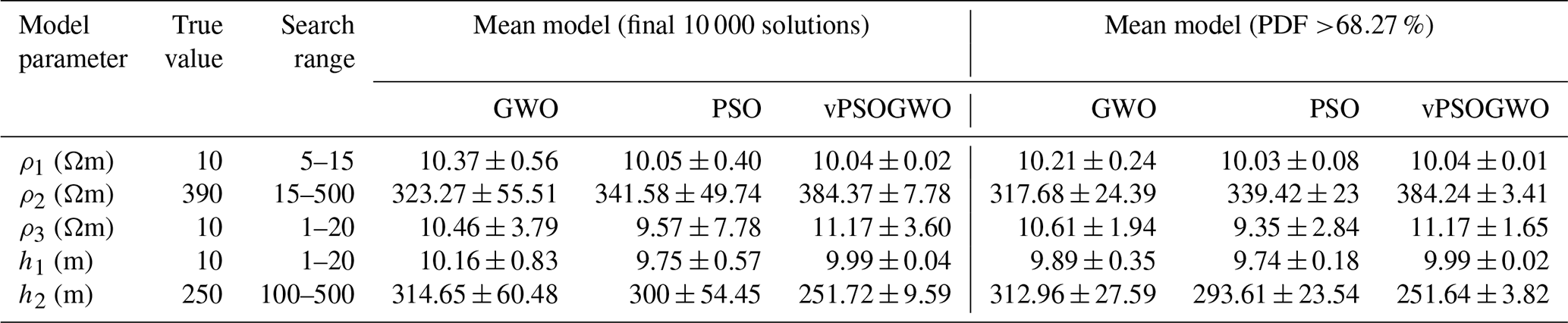
Table 1Optimization of the mean model result for three-layer synthetic resistivity sounding data.
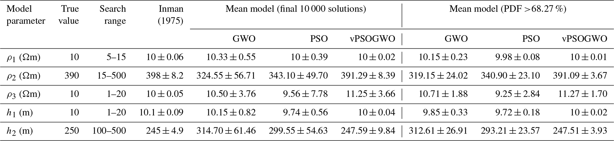
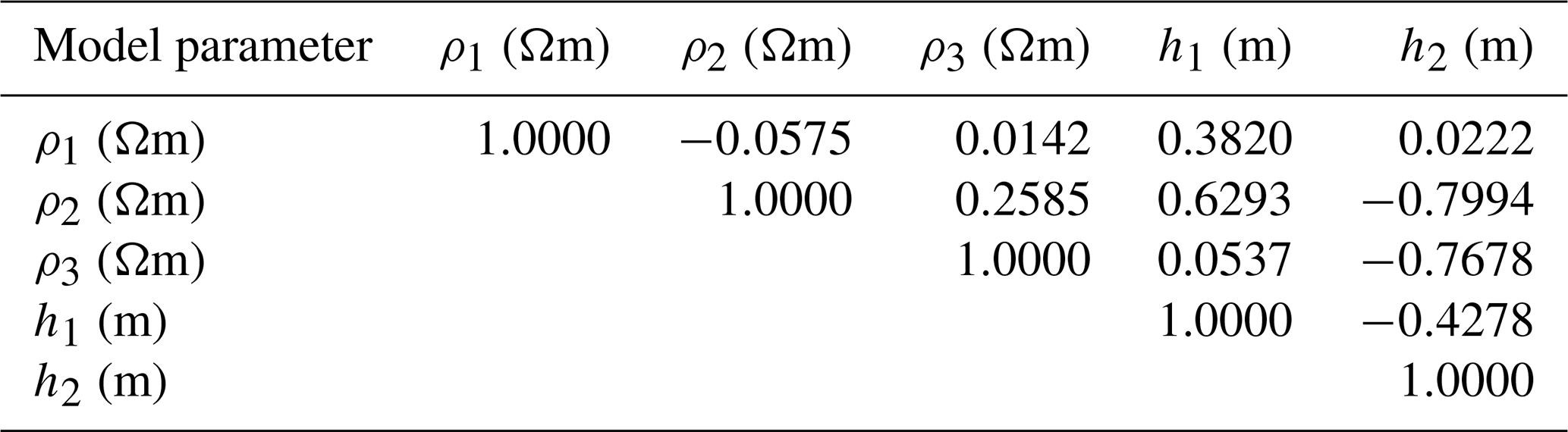
Table 2Correlation matrix using a 68.27 % PDF limit for three-layer synthetic resistivity sounding data.
The proposed algorithms yield good-fitting models, but the evaluation of a global solution requires numerous techniques. This is noteworthy with respect to selecting the region of solution/model search space, where we find enormous solutions. The methods for selecting the region of model space were chosen to envisage the global solution and reduce the uncertainty in the ultimate solution (Mosegaard and Tarantola, 1995; Sen and Stoffa, 1996). Thus, many solutions and the associated error estimated were kept in memory for consequent statistical measurements. Therefore, 108 solutions were generated for each algorithm using the logarithmic mean square error, and every computed response corresponding to each model fits well with the observed response. However, the model parameters obtained, which lie within the search range in multidimensional space, may differ from each other. Hence, the mean model from the model parameters is defined as follows (Ross, 2009):
where i represents the layer parameters, j is the number of models, and mi,j is the jth model with i number of parameters.
All algorithms are executed for 10 000 runs with 1000 iterations to obtain the best model parameters. It is important to mention that multiple runs are crucial in vPSOGWO, as 1000 weightage points lay between the inertial weights of 0.9 and 0.2, such that each weightage point yields a fitted model in a run. As a result, 10 000 runs provide 10 000 chances for each weightage point to fetch the best-fitted model.
Table 3Stability test for three-layer synthetic resistivity sounding data using different search ranges.
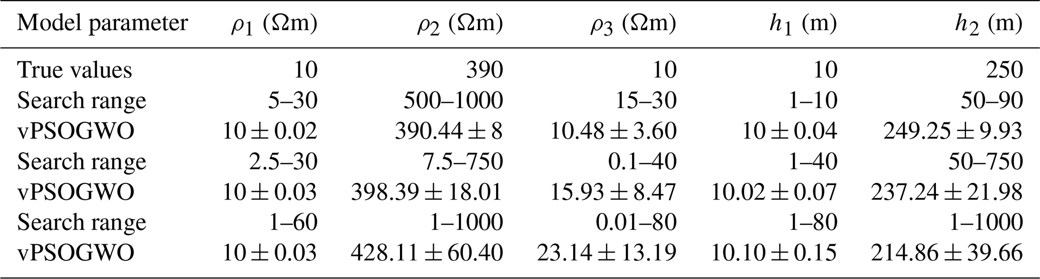
Table 4Optimization mean model result for three-layer synthetic resistivity sounding data with 10 % noise.
Therefore, the posterior covariance matrices are defined using the following equation (Ross, 2009):
Posterior correlation matrices are described using the following equation:
Here, i and k lie between 1 and total number of parameters.
The square roots of the diagonal elements of the covariance matrix define the uncertainty in the solution, and the correlation matrix gives a rough idea about the relation between the model parameters. If the parameters do not provide a global solution, the apparent resistivity curve corresponding to the mean model will not adequate to the observed value. The posterior correlation matrix corresponding to the indigenous solution will not yield an actual correlation between the parameters obtained via linear regression. For further analysis, posterior PDFs and histograms are calculated over all accepted models. The 1D posterior PDF for various parameters with mean and standard deviation σi is given as follows (Ross, 2009):
where y is the solution/model parameter's output store after 10 000 runs of an algorithm and i is between 1 and the number of model parameters.
Different techniques are based on the posterior PDF to obtain the global solution. One of these techniques is to pick the model parameters with the highest probability values. Another method based on the PDF is to normalize (0 to 1) each model parameter by its respective highest probability value. The best model is considered to have the highest sum of normalized probability values (Sharma, 2012). Furthermore, the best model can also be determined by taking the mean of each parameter with probably more significance than the threshold probability. However, these techniques fail to provide the global model.
Therefore, proceeding with a new approach to the study, we introduce a confidence interval (CI) more significant than 68.27 % as a benchmark for all model parameters. According to the empirical rule, 68.27 % of the data lie within 1 standard deviation of the mean (Ross, 2009). Thus, the model parameters below a CI of 68.27 % are discarded, and the remaining parameters are used to determine the mean solution and uncertainty. This means that the model represents the global solution with less uncertainty.
Table 5Correlation matrix using a 68.27 % PDF limit for three-layer synthetic resistivity sounding data with 10 % noise.
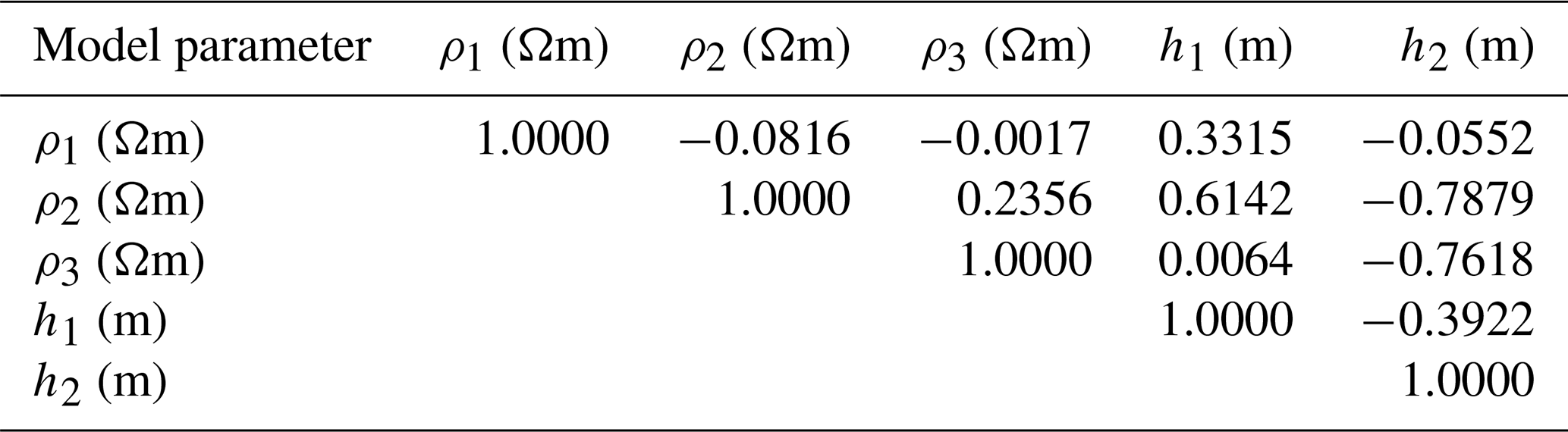
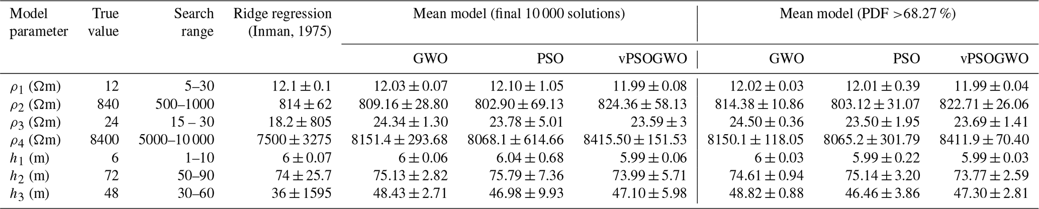
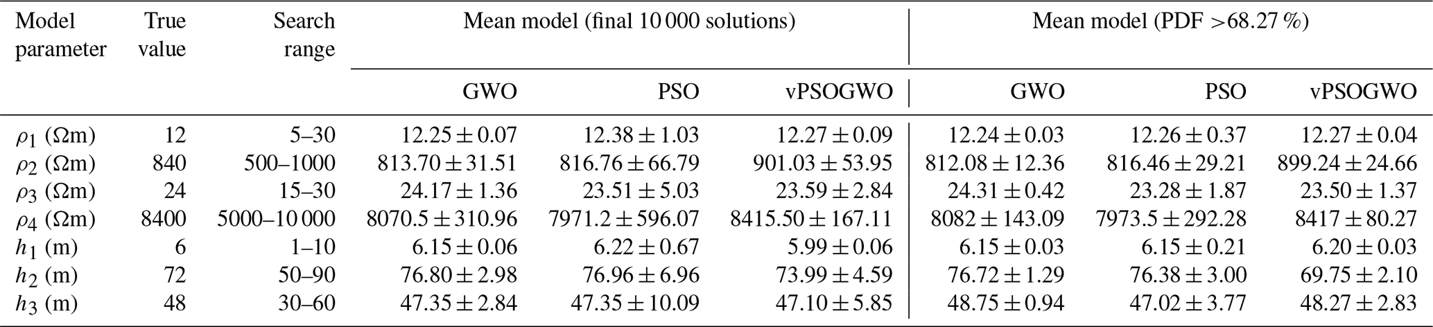
Table 6Optimization of the mean model result for four-layer synthetic resistivity sounding data.
The code used in this work was developed in MATLAB R2019a on a Windows 10 platform with the following configuration: an HP Z240 Tower Workstation and an Intel Xeon E3-1225 v6 3.30 GHz CPU with 32.0 GB of RAM and a 64-bit operating system (OS). However, global optimization is a time-consuming process, as it requires many forwarding calculations to obtain the best-fitted result.
The applicability of the new algorithm (vPSOGWO), GWO, and PSO has been assessed by inverting several cases of synthetic and field data extracted from different geological terrains (Dixon and Doherty, 1977; Panda et al., 2018). Both synthetic and field datasets were computed and optimized using the developed algorithms, maintaining a population size of 10 and 1000 iterations for 10 000 runs, leading each algorithm to analyze 108 models. We discuss the inverted results of the algorithms with respect to their application in a few example synthetic and field cases in the following sections.
6.1 Example 1: synthetic data – three-layer case
Initially, to access the applicability and efficacy of the proposed algorithms, a synthetic apparent resistivity sounding dataset measured with a Schlumberger array was generated considering a three-layer Earth model sandwich with a highly resistant layer of 500.0 Ωm and a thickness of 150.0 m between two low-resistance layers of 8.0 and 5.0 Ωm, respectively. The synthetic data were computed in the MATLAB environment, as shown in Fig. 2a using asterisks. Figure 2a shows the three-layer synthetic data with the best-fitted calculated apparent resistivity curve (>68.27 % PDF), while Fig. 2b presents the 1D mean model (>68.27 % PDF) for the true model (black), vPSOGWO (red), GWO (blue), and PSO (green).
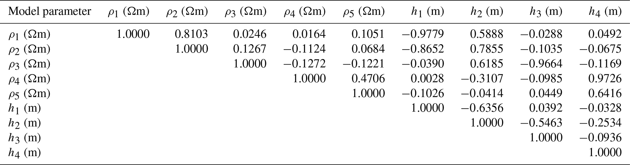
Table 7Correlation matrix using a 68.27 % PDF limit for four-layer synthetic resistivity sounding data.
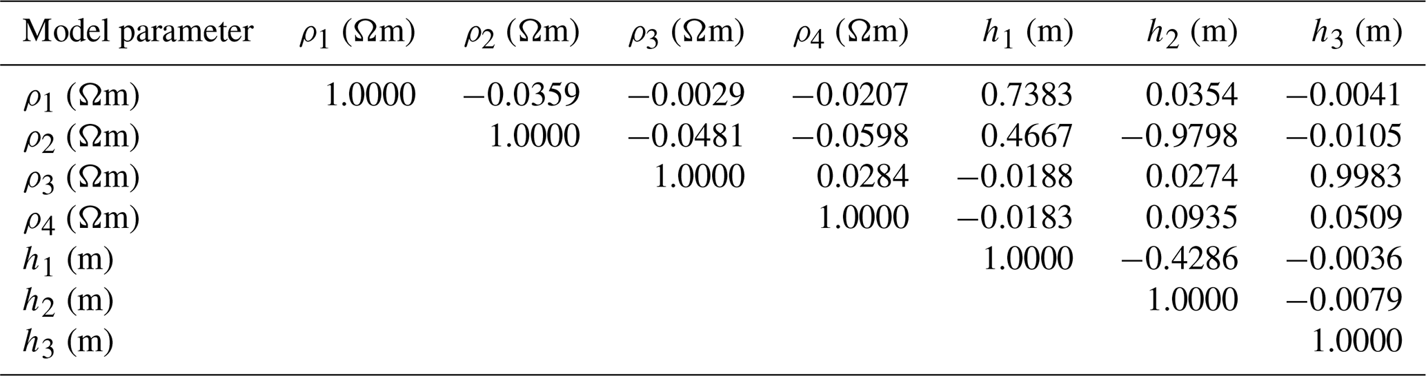
Table 8Optimization of the mean model result for four-layer synthetic resistivity sounding data with 10 % noise.
The search limit for novel inversions techniques (vPSOGWO, GWO, and PSO) is carefully chosen, as shown in Table 1. Each algorithm, including vPSOGWO, runs 10 000 times to perform statistical analysis and determine the global mean model with the least uncertainty. Figure 3 shows the convergence curve of the resistivity layer parameters using vPSOGWO. We found no changes in the convergence pattern after 590 iterations, and layer parameters became stable. The convergence curves, in terms of error versus iterations, for three existing algorithms are shown in Fig. 4. It is observed that vPSOGWO, GWO, and PSO converged at 590, 950, and 380 iterations and have mean square errors of , , and , respectively, whereas ridge regression has an error of 0.633.
The 10 000 models inverted are used to find the posterior PDF and histogram for each parameter. As shown in Fig. 5b, the peak of the posterior PDF is roughly close to the actual model parameter. The histogram shown in Fig. 5a suggests that ρ2 and h2 have a broader range. This represents the equivalence problem associated with the resistive layer, as the uncertainty in each algorithm was found to be large considering all of the accepted models. Therefore, selecting the models with a posterior PDF with a CI greater than 68.27 % reduces the uncertainty in the model, increases the resolution of a solution, and helps estimate the best mean model close to the actual model (Table 1). Table 1 shows the model parameters and uncertainty for the proposed algorithms.
Here, two approaches are used to present the mean solution with its uncertainty estimation: (1) the mean solution for all accepted best-fitted solutions obtained from 10 000 runs for all three algorithms is used or (2) the mean model calculated from the solution with a posterior PDF (for which values are greater than 68.27 % CI from all accepted solution parameters) is used.
Here, we observed that the second-layer parameters for PSO and GWO are too diverted from actual values (higher uncertainty) due to their inability to balance exploitation and exploration properties. In contrast, the hybrid vPSOGWO algorithm provides more accurate results and falls within the uncertainty ranges (Table 1). Therefore, the hybrid algorithm has a more balanced nature with respect to exploitation and exploration than PSO and GWO. As shown in Table 2, the posterior correlation matrix illustrates that the first-layer resistivity reveals a feeble correlation with other associated parameters. However, there is a negative correlation found between ρ2 and h2 (both parameters have a trade-off relationship). In contrast, a positive correlation is observed between ρ2 and h1 (i.e., resistivity of the second layer increases with increasing the thickness of the first layer and vice versa). Similarly, a correlation can also be seen between third-layer resistivity and second-layer thickness, but it is inverse in nature.
Figure 6 represents the correlation plot between model parameters (off-diagonal) and the posterior PDF curve (diagonal) for models with a CI greater than 68.27 % for all parameters. No significant error differences are found between the observed and calculated apparent resistivity data for all three algorithms (Fig. 2a). However, the error difference in the 1D model and the result for the mean model with a CI of 68.27 % are presented in Fig. 2b and Table 1, respectively.
To check the stability of the parameter, the hybrid algorithm is tested with three different search spaces, as shown in Table 3. Consequently, it estimates the mean model and uncertainty for 100 runs. Table 3 suggests that using a broader search space does not cause the result to divert too much from the actual model. In this example, the computational time required for one run with 30 data points was 1.54, 1.49, and 1.48 s for vPSOGWO, GWO, and PSO, respectively.
The proposed optimization is also performed using the same synthetic data with 10 % Gaussian noise and keeping the search range shown in Table 1. The same procedure is applied to determine the mean model from all best-fitted solutions and solutions with a posterior PDF with a CI greater than 68.27 % for parameters of all of the solutions (Table 4). Although 10 % noise is added, the result obtained from the mean model for a posterior PDF of 68.27 % for the hybrid algorithm is not much different compared to actual values. At the same time, the error was observed to slightly increase: , , and for vPSOGWO, GWO, and PSO, respectively. Table 5 depicts the correlation matrix of vPSOGWO, which clearly shows interdependence with values of 0.3315 and −0.7879 for the first- and second-layer parameters. Similarly, we can also determine the relation between second-layer resistivity and first-layer thickness (0.6142), third-layer resistivity, and the second-layer thickness (−0.7618). Hence, the result obtained using the proposed technique shows good agreement with the actual model values.
6.2 Example 2: synthetic data – four-layer case
A four-layer Earth model with a thin, relatively low-resistance layer (24.0 Ωm) sandwiched between two high-resistance layers (840.0 Ωm and 8400.0 Ωm) is considered for the demonstration of the proposed algorithms. Table 6 illustrates the actual model for synthetic data, the search range, and the inverted results. vPSOGWO, GWO, and PSO converge at iterations 590, 674, and 750 and with associated errors of , , and , respectively, as shown in Fig. 8, whereas the error estimated using the ridge regression method is 0.383. Instead of higher error in vPSOGWO compared with GWO, it can be observed that the error scale for the vPSOGWO algorithm is narrower than the other two algorithms, which is an essential factor for determining the mean model (Fig. 9). Hence, the mean model is affected by the error scale, as shown in Fig. 9.
Table 9Correlation matrix using a 68.27 % PDF limit for four-layer synthetic resistivity sounding data with 10 % noise.
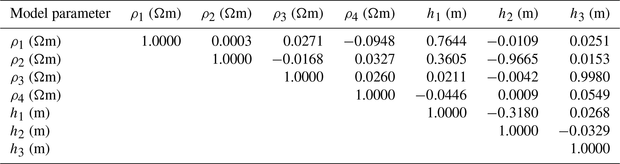
Table 10Optimization of the mean model result for three-layer field resistivity sounding data.
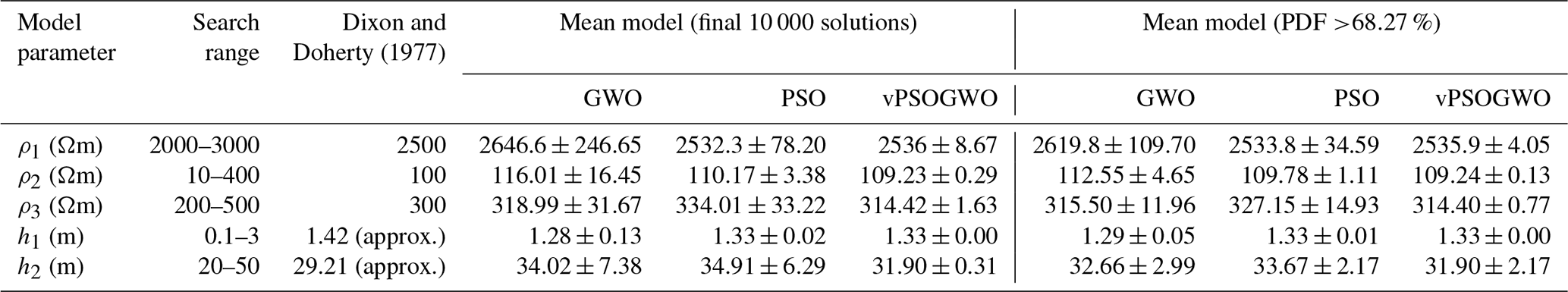
Table 11Correlation matrix using a 68.27 % PDF limit for three-layer field resistivity sounding data.
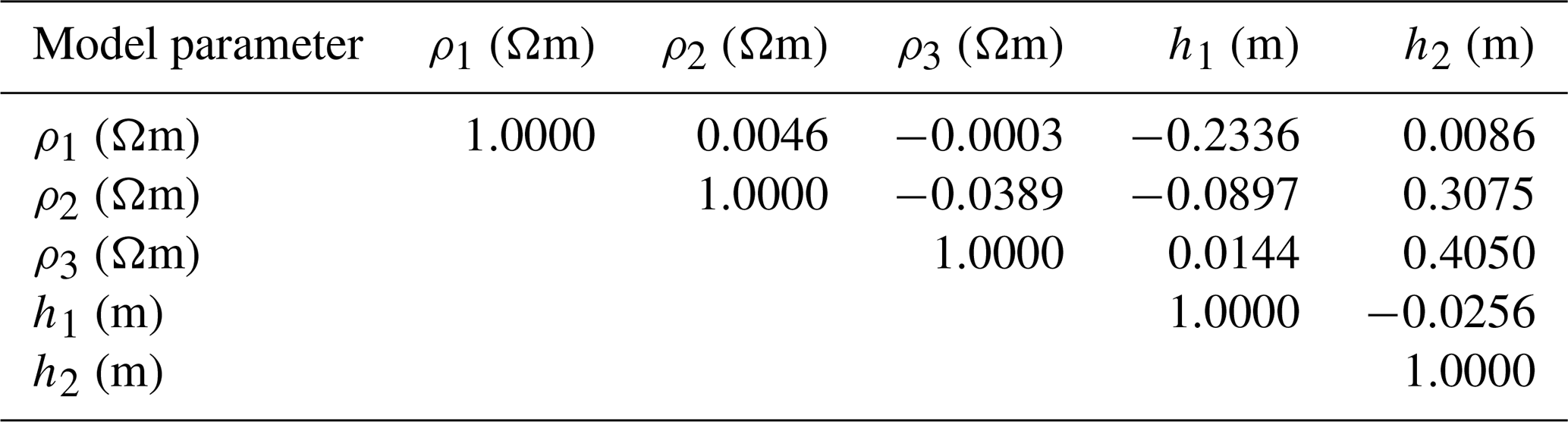
Table 12Optimization of the mean model result for five-layer field resistivity sounding data.
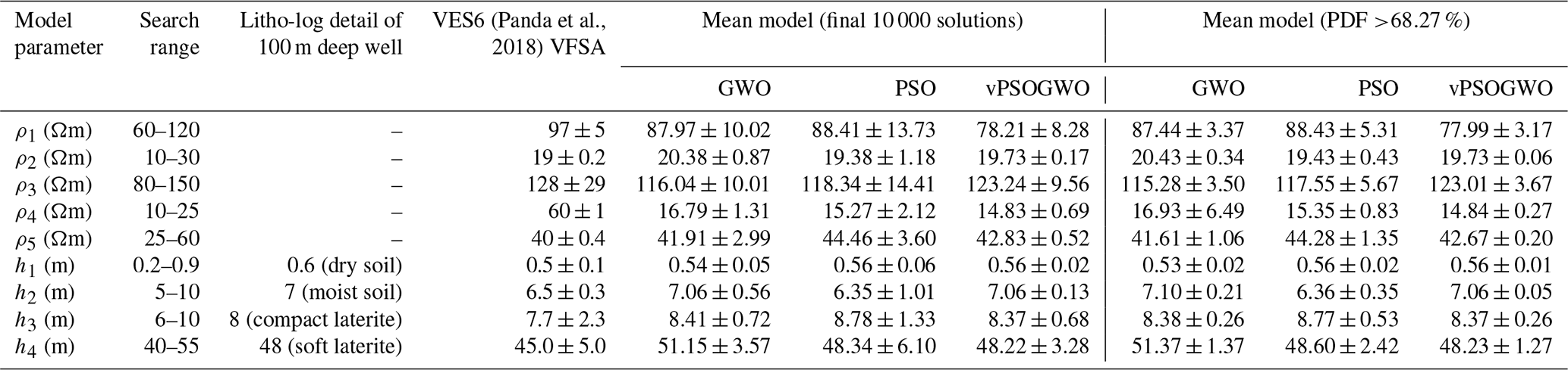
The symbol “–” in the table denotes no information. VFSA stands for very fast simulated annealing.
To reduce uncertainty and increase the resolution of the model, model parameters containing a posterior PDF with a CI greater than 68.27 % are selected. In Table 6, the true model lies within the uncertainty range of the hybrid vPSOGWO, whereas GWO and PSO have failed to keep the true model within its uncertainty range in the second-, third-, and fourth-layer parameters. In the case of ridge regression, the uncertainty level of the model parameters is too high. For example, in the case of the third layer, both resistivity and thickness have an uncertainty approx. 44 times higher than the actual value.
The inverted 10 000 models are also computed in this example to find the posterior PDFs and histograms for each parameter. The peak of the posterior PDF is roughly close to the actual solution, as shown in the histograms in Fig. 10a and b, which reveal that ρ2 and h2 have a broader range that signifies the equivalence problem associated with the resistive layer. The uncertainty in each algorithm is found to be large considering all of the accepted models. However, picking the models with a greater posterior PDF CI than 68.27 % reduces the uncertainty in the model and increases the resolution of a solution.
The correlation plot between model parameters (off-diagonal) and the posterior PDF curve (diagonal) for models with a CI greater than 68.27 % for all parameters is shown in Fig. 11. There are also no significant error differences between the computed and observed apparent resistivity data for all three optimization algorithms.
The correlation matrix of a four-layer model of synthetic resistivity data is shown in Table 7. It illustrates that the first-layer parameters are correlated by a correlation matrix of 0.7383. A strong negative correlation was found between the second-layer parameters (−0.9798), and the third-layer parameters are strongly correlated with each other by a positive correlation matrix of 0.9983. Figure 7a shows the fitness between four-layer synthetic (*) and computed apparent resistivity data obtained for vPSOGWO, GWO, and PSO. The difference in fitness curves for all three optimization techniques cannot be determined, as the observed error is significantly negligible. However, the error difference can be observed in the 1D resistivity–depth models obtained from the mean model with a PDF CI of 68.27 %, as shown in Fig. 7b. Table 6 shows the mean model with a posterior PDF with a CI greater than 68.27 % for all accepted parameters in the four-layer Earth model case. In this example, the computational time required for one run with 27 data points for vPSOGWO, GWO, and PSO is 1.94, 1.84, and 1.85 s (PSO), respectively.
The optimization techniques are also executed using the same four-layer model of synthetic data with 10 % Gaussian noise and keeping the search range shown in Table 6. The same procedure is applied to determine the mean model from all of the best-fitted models and models of a posterior PDF with a CI greater than 68.27 % for all model parameters presented in Table 8. Although 10 % noise is added, the result obtained from the mean model for the posterior PDF CI of 68.27 % for the hybrid algorithm is not much different from actual values. At the same time, the experimental error is , , and for vPSOGWO, GWO, and PSO, respectively.
Table 9 illustrates the correlation matrix of the hybrid algorithm, which clearly describes interdependence, as seen by values of 0.7644, −0.9665, and 0.9980 for the first- and second-, and third-layer parameters, respectively. Similarly, we also find a relation between second-layer resistivity and first-layer thickness (0.3605) and the resistivity of the fourth layer and thickness of the third layer (0.0549). This means that the outcome from the advocated proposed is very close to the real model.
6.3 Example 3: field data – three-layer case
For the first field example, we used a one three-layer case of vertical electrical resistivity sounding data measured with a Schlumberger array over Mount Turner, northern Queensland, Australia, interpreted by Dixon and Doherty (1977, Fig. 2a), as shown in Fig. 12a. After selecting a suitable search range, three novel algorithms, namely, vPSOGWO, GWO, and PSO, are executed to reconstruct the model interpreted by Dixon and Doherty (1977). The search range and the comparison of the proposed algorithms with the previous result (Dixon and Doherty, 1977) are presented in Table 10. Our results (for a 68.27 % CI) are closed to the development given by Dixon and Doherty (1977). The convergent error for the best-fitted model in vPSOGWO is , GWO is , and PSO is .
Table 11 presents a correlation matrix that shows a negative correlation between the first-layer parameters and a positive correlation between the second-layer parameters. A positive correlation is also observed between ρ3 and h2, which maintain the same model data. Figure 12a shows the apparent resistivity curve, while the 1D model obtained from the mean model with a 68.27 % CI result is shown in Fig. 12b. In this example, the computational time required for one run with 14 data points is 0.90, 0.83, and 0.78 s for vPSOGWO, GWO, and PSO respectively.
6.4 Example 4: field data – five-layer case
We selected another field example using a vertical electrical resistivity sounding dataset from Keshiari (Kharagpur), West Bengal, India, as a five-layer Earth subsurface model to determine the aquifer zone (Panda et al., 2018, their Fig. 3). This area is covered with different geological units, such as laterite, clay, and sand, and laterite material restricts the aquifer recharge process and is the most problematic area with respect to groundwater potential. We inverted these data for a five-layer Earth structure parameter using the vPSOGWO, GWO, and PSO inversion algorithms. The results are shown in Table 12 for the available models, borehole samples, and the search space for vPSOGWO, GWO, and PSO. The computed apparent resistivity curve for all three algorithms (–) and the field data (indicated by asterisks) are shown in Fig. 13a. Their error differences are significant (Fig. 13a, Table 12). The inverted 1D layered model using all algorithms obtained from the mean model with a 68.27 % CI is shown in Fig. 13b. In this example, the computational time for one run with 28 data points is 2.55, 2.43, and 2.45 s for vPSOGWO, GWO, and PSO, respectively.
Table 13Correlation matrix using a 68.27 % PDF limit for five-layer field resistivity sounding data.
The result obtained from the mean solution of all accepted solutions and solutions with a PDF CI greater than 68.27 % aimed at all parameters using the developed techniques is presented in Table 12. The final mean models are comparable with lithological data from a 100 m deep tube well near VES6. The convergent error for vPSOGWO, GWO, and PSO is , , and , respectively, whereas the error for very fast simulated annealing (VFSA) obtained by Panda et al. (2018) is . The correlation matrix clearly shows a strong relation between the parameters of the first layer (−0.9736), the second layer (0.8434), and the third layer (−0.9907) as well as a moderate relation between the parameters of the fourth layer (0.5653). We have noticed a moderate interdependence of ρ3 with h2 and of ρ5 with h4, which can be seen in Table 13.
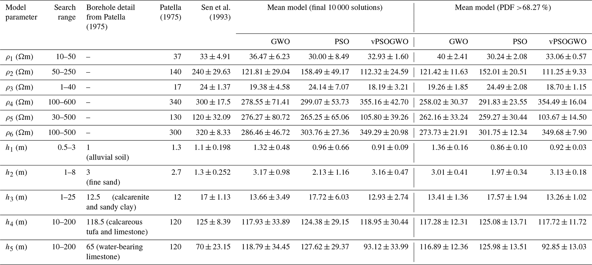
Table 14Optimization of the mean model result for six-layer field resistivity sounding data.
6.5 Example 5: field data – six-layer case
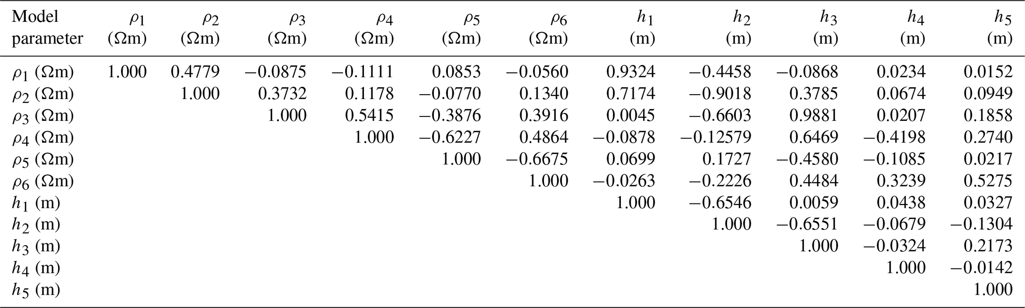
As a six-layer case study, we again applied the vPSOGWO, GWO, and PSO algorithms to invert field apparent resistivity data extracted near a borehole in Apulia, South Italy, for hydrogeological purposes (Sen et al., 1993). The search range was taken from Sen et al. (1993), but the fourth-layer and upper-bound thickness of the fifth layer increase by 50 m, as shown in Table 14. The reproduced field data (*) and inverted field data (–) are shown in Fig. 14a. The misfit error obtained is , , and for vPSOGWO, GWO, and PSO, respectively, whereas the error using simulating annealing (SA) in Sen et al. (1993) is 0.017. Table 14 also includes the mean model for a CI of 100 % and 68.27 % using the proposed algorithms and previously published literature. It is observed that few parameters obtained fall within the uncertainty of corresponding parameters of vPSOGWO. The vPSOGWO-inverted results provide higher similarity with the borehole information than the results from SA (Sen et al., 1993). The interdependence between the layer parameters can be seen from the correlation matrix shown in Table 15. A strong correlation among parameters of the first layer (0.8211), the second layer (−0.9327), and the third layer (0.9766) is shown by the correlation matrix, which is comparable to the correlation matrix that has been presented in Sen et al. (1933, their Table 13). A moderate correlation between fourth-layer (−0.5246) and fifth-layer parameters (0.4486) is also observed. It is also notable that there is a sensible relation between sixth-layer resistivity and fifth-layer thickness, keeping the same model data.
The error differences between computed data and observed data are significant, as shown in Fig. 14a and Table 12. The inverted 1D layered models obtained from the mean model with a CI of 68.27 % are shown in Fig. 14b. In this example, the computational time for one run with 28 data points is 3.58, 3.44, and 3.45 s for vPSOGWO, GWO, and PSO, respectively. The inverted results from vPSOGWO, GWO, and PSO have been shown along with the borehole data and published results (Sen et al., 1993) in Table 14. In addition to published findings, it is notable that the outcomes obtained from the hybrid algorithm (vPSOGWO) satisfy the borehole information very well compared with the other algorithms.
Table 15Correlation matrix using a 68.27 % PDF limit for six-layer field resistivity sounding data.
We conducted an assessment of three metaheuristic algorithms, namely PSO, GWO, and vPSOGWO, to determine their effectiveness and suitability with respect to solving geoelectrical inverse issues. These challenges include the estimation of 1D resistivity models based on geoelectrical resistivity sounding data. The relevance of these algorithms was validated using synthetic and field resistivity sounding data signifying the different kinds of Earth subsurface stratigraphy. An enormous solution (100 000 000 from 10 000 runs) was assessed. Subsequently, the best-fitted solutions were chosen within a predefined value for statistical measurements. The statistical study, including a posterior PDF with a 68.27 % CI, a mean solution, a posterior solution correlation matrix, and a covariance matrix using search space, was carried out to refine the solutions and obtain the global mean solution with the least uncertainty. These statistical simulations yield essential information as to the reliability of an inversion algorithm. In general, conventional techniques can be quite effective in resolving the model with respect to random noise but can fail with respect to systematic error and inappropriate models. Our investigation with the application of the developed algorithm, including the statistical simulation for different multilayer resistivity parameters, resulted in a quantitative appraisal of uncertainty in the derived model parameters. We observed that the output of the hybrid algorithm in terms of the mean model or error might be similar to either PSO or GWO (attributed to the exploration characteristics of GWO and the exploitation characteristics of PSO). The vPSOGWO, GWO, and PSO algorithm performance has been analyzed based on the uncertainty and stability and on the mean model of the layered Earth structure. We found that vPSOGWO gives much closer results than the results inverted from other two algorithms and than conventional methods and that these results are consistently better than the previously published results and are correlated well with borehole information.
The data supporting the findings of this study can be made available from corresponding author upon request. All data utilized to demonstrate our developed algorithms are published/public domain data or are presented in the tables and figures in this paper.
KS: conceptualization of the study, methodology, computer code, analysis, and drafting of the manuscript; UKS: supervision, suggestions, and editing; JVT: drafting and editing of the manuscript and algorithm validation.
The contact author has declared that neither of the authors has any competing interests.
Publisher’s note: Copernicus Publications remains neutral with regard to jurisdictional claims made in the text, published maps, institutional affiliations, or any other geographical representation in this paper. While Copernicus Publications makes every effort to include appropriate place names, the final responsibility lies with the authors.
The authors would like to express their gratitude to the IIT (ISM), Dhanbad, for providing a pleasant environment and financial support to pursue this study. We also express our thankful to the chief editor, associate editor, and anonymous reviewers, whose suggestions and comments enabled us to better understand the issues and considerably improve our manuscript.
This research has been supported by the Indian Institute of Technology (Indian School of Mines), Dhanbad (https://www.iitism.ac.in, last access: 5 December 2023).
This paper was edited by Christian Franzke and reviewed by Khalid Essa and Stanley Raj.
Colorni, A., Dorigo, M., and Maniezzo, V.: Distributed optimization by ant colonies, in: Proceedings of the first European conference on artificial life, 142, 134–142, https://faculty.washington.edu/paymana/swarm/colorni92-ecal.pdf (last access: 14 December 2023), 1991.
Dixon, O. and Doherty, J. E.: New interpretation methods for IP soundings, Explor. Geophys., 8, 65–69, https://doi.org/10.1071/EG977065, 1977.
Eiben, A. E. and Schippers, C. A.: On evolutionary exploration and exploitation, Fundam. Inform., 35, 35–50, https://doi.org/10.3233/FI-1998-35123403, 1998.
Esmin, A. A. and Matwin, S.: HPSOM: a hybrid particle swarm optimization algorithm with genetic mutation, Int. J. Innov. Comput. I., 9, 1919–1934, 2013.
Inman, J. R.: Resistivity inversion with ridge regression, Geophysics, 40, 798–817, https://doi.org/10.1190/1.1440569, 1975.
Kennedy, J. and Eberhart, R.: Particle swarm optimization. In Proceedings of ICNN'95 – International Conference on Neural Networks IEEE 4, Perth, WA, Australia, 27 November 1995–1 December 1995, 1942–1948, https://doi.org/10.1109/ICNN.1995.488968, 1995.
Koefoed, O.: Geosounding principles, 1: Resistivity sounding measurements. Methods in Geochemistry and Geophysics: Elsevier Science Ltd. Co., Amsterdam, 14A, pp. 276, ISBN 0444417044, 9780444417046, 1979.
Kamboj, V. K.: A novel hybrid PSO–GWO approach for unit commitment Problem, Neural Comput. Appl., 27, 1643–1655, https://doi.org/10.1007/s00521-015-1962-4, 2015.
Lai, X. and Zhang, M.: An efficient ensemble of GA and PSO for real function optimization, in: 2009 2nd IEEE International Conference on Computer Science and Information Technology, IEEE, Beijing, China, 8–11 August 2009, 651–655, https://doi.org/10.1109/ICCIA.2010.6141614, 2009.
Mirjalili, S. and Hashim, S. Z. M.: A new hybrid PSOGSA algorithm for function optimization, in: 2010 International conference on computer and information application, IEEE, Tianjin, China, 3–5 December 2010, 374–377, https://doi.org/10.1109/ICCIA.2010.6141614, 2010.
Mirjalili, S., Mirjalili, S. M., and Lewis, A.: Grey wolf optimizer, Adv. Eng. Softw., 69, 46–61, https://doi.org/10.1016/j.advengsoft.2013.12.007, 2014.
Mitchell, M.: An introduction to genetic algorithms. A Bradford Book, The MIT Press, 1998.
Mosegaard, K. and Tarantola, A.: Monte Carlo sampling of solutions to inverse problems, J. Geophys. Res.-Atmos., 100, 12431–12448, https://doi.org/10.1029/94JB03097, 1995.
Narayan, S., Dusseault, M. B., and Nobes, D. C.: Inversion techniques applied to resistivity inverse problems, Inverse Probl., 10, 669–686, https://doi.org/10.1088/0266-5611/10/3/011, 1994.
Oldenburg, D. W. and Li, Y.: Inversion of induced polarization data, Geophysics, 59, 1327–1341, https://doi.org/10.1190/1.1443692, 1994.
Panda, K. P., Sharma, S. P., and Jha, M. K.: Mapping lithological variations in a river basin of West Bengal, India using electrical resistivity survey implications for artificial recharge, Environ. Earth Sci., 77, 626, https://doi.org/10.1007/s12665-018-7813-8, 2018.
Patella, D.: A numerical computation procedure for the direct interpretation of geoelectrical soundings, Geophys. Prospect., 23, 335–362, https://doi.org/10.1111/j.1365-2478.1975.tb01533.x, 1975.
Pekeris, C. L.: Direct method of interpretation in resistivity prospecting, Geophysics, 5, 31–42, https://doi.org/10.1190/1.1441791, 1940.
Rashedi, E., Nezamabadi-Pour, H., and Saryazdi, S.: GSA: a gravitational search algorithm, Inform. Sciences, 179, 2232–2248, https://doi.org/10.1016/j.ins.2009.03.004, 2009.
Roshan, R. and Singh, U. K.: Inversion of residual gravity anomalies using tuned PSO, Geosci. Instrum. Method. Data Syst., 6, 71–79, https://doi.org/10.5194/gi-6-71-2017, 2017.
Ross, S.: Probability and statistics for engineers and scientists, Elsevier, New Delhi, 16, 32–33, 2009.
Sen, M. K. and Stoffa, P. L.: Bayesian inference, Gibbs' sampler and uncertainty estimation in geophysical inversion, Geophys. Prospect., 44, 313–350, https://doi.org/10.1111/j.1365-2478.1996.tb00152.x, 1996.
Sen, M. K., Bhattacharya, B. B., and Stoffa, P. L.: Nonlinear inversion of resistivity sounding data, Geophysics, 58, 496–507, https://doi.org/10.1190/1.1443432, 1993.
Şenel, F. A., Gökçe, F., Yüksel, A. S., and Yiğit, T.: A novel hybrid PSO–GWO algorithm for optimization problems, Eng. Comput., 35, 1359–1373, https://doi.org/10.1007/s00366-018-0668-5, 2019.
Sharma, S. P.: VFSARES – a very fast simulated annealing FORTRAN program for interpretation of 1-D DC resistivity sounding data from various electrode arrays, Comput. Geosci., 42, 177–188, https://doi.org/10.1016/j.cageo.2011.08.029, 2012.
Simon, D.: Biogeography-based optimization, IEEE T. Evolut. Comput., 12, 702–713, https://doi.org/10.1109/TEVC.2008.919004, 2008.
Singh, N. and Singh, S. B.: Hybrid algorithm of particle swarm optimization and grey wolf optimizer for improving convergence performance, J. Appl. Math., 2017, 2030489, https://doi.org/10.1155/2017/2030489, 2017.
Singh, U. K., Tiwari, R. K., and Singh, S. B.: One-dimensional inversion of geo-electrical resistivity sounding data using artificial neural networks – a case study, Comput. Geosci., 31, 99–108, https://doi.org/10.1016/j.cageo.2004.09.014, 2005.
Singh, U. K., Tiwari, R. K., and Singh, S. B.: Neural network modeling and prediction of resistivity structures using VES Schlumberger data over a geothermal area, Comput. Geosci., 52, 246–257, https://doi.org/10.1016/j.cageo.2012.09.018, 2013.
Storn, R. and Price, K.: Differential evolution – a simple and efficient heuristic for global optimization over continuous spaces, J. Global Optim., 11, 341–359, https://doi.org/10.1023/A:1008202821328, 1997.
Whitley, D.: A genetic algorithm tutorial, Stat. Comput., 4, 65–85, https://doi.org/10.1007/BF00175354, 1994.
Yang, X. S.: A new metaheuristic bat-inspired algorithm, in: Nature inspired cooperative strategies for optimization (NICSO 2010), Springer, Berlin, Heidelberg, 65–74, https://doi.org/10.1007/978-3-642-12538-6_6, 2010.
- Abstract
- Introduction
- Forward modeling algorithm
- Inverse modeling algorithm
- Statistical simulation for global model and uncertainty estimation
- Computational information
- Results and discussion
- Conclusion
- Data availability
- Author contributions
- Competing interests
- Disclaimer
- Acknowledgements
- Financial support
- Review statement
- References