A global analysis of the fractal properties of clouds revealing anisotropy of turbulence across scales

The deterministic motions of clouds and turbulence, despite their chaotic nature, have nonetheless been shown to follow simple statistical power-law scalings: a fractal dimension D relates individual cloud perimeters p to a measurement resolution, and turbulent fluctuations scale with the air parcel separation distance through the Hurst exponent, ℋ. However, it remains uncertain whether atmospheric turbulence is best characterized by a split isotropy that is three-dimensional (3D) with $\mathcal{H}=\mathrm{1}/\mathrm{3}$ at small scales and two-dimensional (2D) with ℋ=1 at large scales or by a wide-range anisotropic scaling with an intermediate value of ℋ. Here, we introduce an “ensemble fractal dimension” D_e – analogous to D – that relates the total cloud perimeter per domain area 𝒫 as seen from space to the measurement resolution, and we show theoretically how turbulent dimensionality and cloud edge geometry can be linked through $\mathcal{H}=D_e-\mathrm{1}$. Observationally and numerically, we find the scaling $D_e\sim \mathrm{5}/\mathrm{3}$ or $\mathcal{H}\sim \mathrm{2}/\mathrm{3}$, spanning 5 orders of magnitude of scale. Remarkably, the same scaling relationship links two “limiting case” estimates of 𝒫 evaluated at resolutions corresponding to the planetary scale and the Kolmogorov microscale, which span 10 orders of magnitude. Our results are nearly consistent with a previously proposed “23/9D” anisotropic turbulent scaling and suggest that the geometric characteristics of clouds and turbulence in the atmosphere can be easily tied to well-known planetary physical parameters.

1 Introduction

The Earth system is radiatively open and materially closed. Radiatively, Earth's global mean temperature is sustained by a balance between absorption of high-intensity shortwave sunlight and the reemission at longwave frequencies to the cold of space. Materially, the total dry atmospheric mass is confined to the planet by gravity and can only be redistributed by turbulent circulations that mix air over a broad range of scales within the thin atmospheric layer. Clouds play important roles in determining the magnitude of both categories of flow. Geometrically speaking, cloud areas govern radiative fluxes (Zelinka et al., 2022), while the edge length or perimeter of clouds controls material exchanges of air between clouds and their clear-sky environment (Zhao and Austin, 2005; Heus et al., 2008; Garrett et al., 2018).

A scientific challenge is that the seemingly objective properties of cloud area and perimeter are a function of the more subjective choice of spatial resolution, ξ (defined as either the pixel side-length in a satellite image or the grid spacing in a model). Clouds smaller than ξ cannot be resolved, and the square shapes in a resolved grid do not reflect more irregular cloud structures. Even casual observations of the sky show cloud edges that are intricately complex for any plausibly resolvable scale. For example, the boundary of a small cumulus cloud may appear smoothly rounded at first glance, but fine turbulent structures become apparent when it is viewed through binoculars. The change in the observational scale lengthens the cloud boundary with clear skies even as the total cloud area remains nearly unchanged. Because the resolution-dependent cloud perimeter is shaped by the complex and chaotic processes of turbulent mixing and diffusion (Hentschel and Procaccia, 1984) and while air and energy exchanges are physically independent of ξ, a resolution-based link is required to relate the two (Lovejoy et al., 2001; Fielding et al., 2020).

Fractal geometry is often used as a tool for characterizing the resolution-dependent complexity of shapes. The fractal dimension D was first introduced by Richardson (1961) to characterize the complexity of political borders and was later popularized by Mandelbrot (1967) to describe how the length of a coastline changes depending on the length of the ruler used to measure it. Generally, the perimeter p around an individual fractal object can be related to the measurement resolution ξ through

$$\begin{array}{}\text{(1)}& p\propto {\mathit{\xi }}^{\mathrm{1}-D}.\end{array}$$

For the Euclidean case that p is independent of ξ, then D=1. At the other extreme, a “space-filling” curve that passes through every resolved point in a unit area has D=2. Lovejoy (1982) first measured D for clouds by relating individual cloud perimeters p to cloud areas a using the expression $p\propto {\sqrt{a}}^D$. A measured value of $D=\mathrm{1.35}\pm \mathrm{0.05}\approx \mathrm{4}/\mathrm{3}$ has since been adopted as the canonical value describing individual clouds (Siebesma and Jonker, 2000; Christensen and Driver, 2021) although various studies have shown that D can vary considerably from cloud to cloud. For example, Batista-Tomás et al. (2016) found distinct fractal dimension values for cirrus clouds with ragged, tenuous edges of D=1.37, whereas for cumulonimbus clouds with smoother edges, D=1.18. Other analyses of cumulus fields have found values of D=1.28 (Zhao and Di Girolamo, 2007) and D=1.19 (Mieslinger et al., 2019), which were determined using the expression $p\propto {\sqrt{a}}^D$.

Generally, we define here a geometric quantity that does not vary with the length scale as “scale-invariant” such as the scaling of p with ξ in Eq. (1) does. For such scale invariance to apply to an atmospheric cloud field, this would require that the physics controlling cloud shapes is unchanged with measurement resolution, at least between the limits of possible cloud sizes. Clouds have been shown to be broadly scale-invariant for the number distributions of cloud areas and perimeters (DeWitt et al., 2024) despite previous observations of scale breaks that appeared to separate small and large clouds into different physical regimes. DeWitt and Garrett (2024) argue that these scale breaks are artifacts that owe to the treatment of clouds that are truncated by the edge of the measurement domain.

Although the initial result of Lovejoy (1982) showed a constant value of D for length scales ranging from 1 to 1000 km, suggesting a wide-ranging scale invariance of clouds, the value of D has sometimes been observed to be greater for larger clouds. Cahalan and Joseph (1989) reported that D=1.27 for small clouds and D=1.56 for large clouds, which was supported by Benner and Curry (1998), who found that D=1.23 and D=1.34, respectively. Furthermore, after reexamining the data in Lovejoy (1982), Gifford (1989) noted that D increases from 1.35 to 1.77 for the largest clouds with areas $>\mathrm{2.5}\times {\mathrm{10}}^{\mathrm{4}}$ km². The apparent increase in measured D for larger clouds suggests a violation of scale invariance. However, this is likely another artifact of the data analysis methods. The inclusion of interior cloud holes in area and perimeter measurements has been shown to overestimate calculations of D using the expression $p\propto {\sqrt{a}}^D$ (Peters et al., 2009; Brinkhoff et al., 2015). Because interior holes tend to fill when imaged with an increasingly coarse resolution, this ξ dependence of a results in an inaccurate value of D – the error in which can be calculated using multifractal analysis (Lovejoy and Schertzer, 1991).

Clouds have been shown to be multifractal; i.e., D is a continuous function of the threshold used to distinguish clouds from clear skies (Lovejoy and Schertzer, 1990, 1991; Marshak et al., 1995; Lovejoy and Schertzer, 2006). Studies of the multifractal properties of clouds are useful because they can be used to mathematically account for turbulent intermittency (the variability in turbulent fluctuations), which is notably observed in measurements of the water mixing ratio (Tuck, 2022). We argue that a monofractal assumption is sufficient for the primary conclusions of this study in Sect. 5.4.

While the fractal dimension and scale invariance are intrinsically linked, their relationship with turbulent structures in the atmosphere is less clear. Two paradigms of turbulence scaling in the atmosphere have been the topic of decades of debate: split 2D and 3D isotropic scaling regimes for large and small scales (Fiedler and Panofsky, 1970; Nastrom et al., 1984) and wide-ranging anisotropic scaling (Lovejoy, 2023). Both theories originated from the pioneering work of Richardson (1926), who showed that the turbulent eddy diffusivity K, measured using the relative motion of pairs of particles separated by distance ℓ, followed a power law with a $\mathrm{4}/\mathrm{3}$ exponent from the millimeter scale for molecular diffusion to the length scale of atmospheric cyclones (ℓ∼10³ km), $K\propto {\mathrm{\ell }}^{\mathrm{4}/\mathrm{3}}$, termed the Richardson “$\mathrm{4}/\mathrm{3}$ law” of atmospheric diffusion.

The scaling exponent of the diffusivity with respect to the length scale can be experimentally obtained from measurements of velocity fluctuations, Δv, of two air parcels separated by a distance ℓ using passive scalars Θ as a physical quantity that is affected by but does not affect the turbulent flow such as the concentration of aerosols (Celani et al., 2002). Along one dimension x, the generalized first-order “structure function” (which ignores intermittency) expresses the covariance of Θ as a function of separation distance, ℓ. For turbulent scalars, the function tends to be a power law given by

$$\begin{array}{}\text{(2)}& S\left(\mathrm{\ell }\right)=\left|\mathrm{\Delta }\mathrm{\Theta }\right(\mathrm{\ell }\left)\right|=〈\left|\mathrm{\Theta }\right(x+\mathrm{\ell })-\mathrm{\Theta }(x\left)\right|〉\propto {\mathrm{\ell }}^{\mathcal{H}},\end{array}$$

where brackets indicate averaging over many iterations of the experiment and ℋ is the Hurst exponent¹, with bounds $\mathrm{0}<\mathcal{H}<\mathrm{1}$ (Schertzer and Lovejoy, 1983; Hentschel and Procaccia, 1984; Lovejoy and Schertzer, 2012).

The $\mathrm{4}/\mathrm{3}$ law was later derived using dimensional reasoning applied to the theory of 3D isotropic turbulence developed by Kolmogorov (1941). In the theory, for a fluid with kinematic viscosity ν, turbulence kinetic energy is passed along an energy cascade, from large eddies of the energy input scale, L, to progressively smaller eddies with a constant kinetic energy dissipation rate ε, ending at the Kolmogorov microscale, $\mathit{\eta }\sim ({\mathit{\nu }}^{\mathrm{3}}/\mathit{\epsilon }{)}^{\mathrm{4}}\sim \mathrm{1}$ mm, a dissipation length scale where inertial and viscous forces are in balance. Through dimensional analysis, the covariance of air parcel velocity fluctuations was derived to be $\mathrm{\Delta }v\approx {\mathit{\epsilon }}^{\mathrm{1}/\mathrm{3}}{\mathrm{\ell }}^{\mathcal{H}}$, where $\mathcal{H}=\mathrm{1}/\mathrm{3}$ for the case of 3D isotropic turbulence. The dimensional approximation that K∼ℓv (Tennekes and Lumley, 1972) results in $K\sim {\mathit{\epsilon }}^{\mathrm{1}/\mathrm{3}}{\mathrm{\ell }}^{\mathrm{4}/\mathrm{3}}$, reproducing Richardson's $\mathrm{4}/\mathrm{3}$ power law, and implying that the relationship between diffusivity and the Hurst exponent ℋ (again ignoring intermittency), follows

$$\begin{array}{}\text{(3)}& K\sim {\mathrm{\ell }}^{\mathrm{1}+\mathcal{H}}.\end{array}$$

As Sect. 5 elaborates, the value of ℋ differs based on the dimensionality of the turbulence (e.g., the case of 2D isotropic turbulence). The problem that 3D turbulence cannot apply at the “flatter” planetary scales to a relatively thin troposphere is well known. Even Kolmogorov predicted that 3D turbulence can only apply in the atmosphere at scales <100 m. This led to the paradigm that 3D isotropic turbulence must be applicable at small scales and 2D at large scales, separated by a scale break around the depth of the troposphere (see Lovejoy, 2023, for a historical review). The contrasting case for 2D turbulence was developed for the case of an incompressible fluid (Kraichnan, 1967) and later refined into the theory of 2D quasi-geostrophic turbulence (Charney, 1971), where the expected value is instead ℋ=1.

Figure 1 illustrates how two- and three-dimensional (2D and 3D) components in cloud structures are visible at all scales, but, arguably, 2D structures predominate at scale L, becoming more 3D approaching η, reflecting a scale dependence due to large-scale stratification. Aircraft measurements of turbulent spectra of wind and temperature fluctuations have been argued to support this physical separation of large and small scales, where quasi-2D structures are seen at large scales and isotropic 3D structures at small scales (Fiedler and Panofsky, 1970), with a scale break seen between approximately 20 and 500 km (Nastrom et al., 1984; Gage and Nastrom, 1986). Lovejoy et al. (2009) argued that this scale break is an artifact owing to vertical aircraft movements that occur when flying along isobars rather than isoheights and proposed instead that 3D isotropic turbulence is inapplicable at nearly any scale because stratification compresses the atmosphere vertically, even for scales as small as 5 m. Furthermore, the results of Alder and Wainwright (1970) show the formation of vortices even at the 10⁻⁸ m scale, inconsistent with a description of isotropic molecular diffusion (Tuck, 2022).

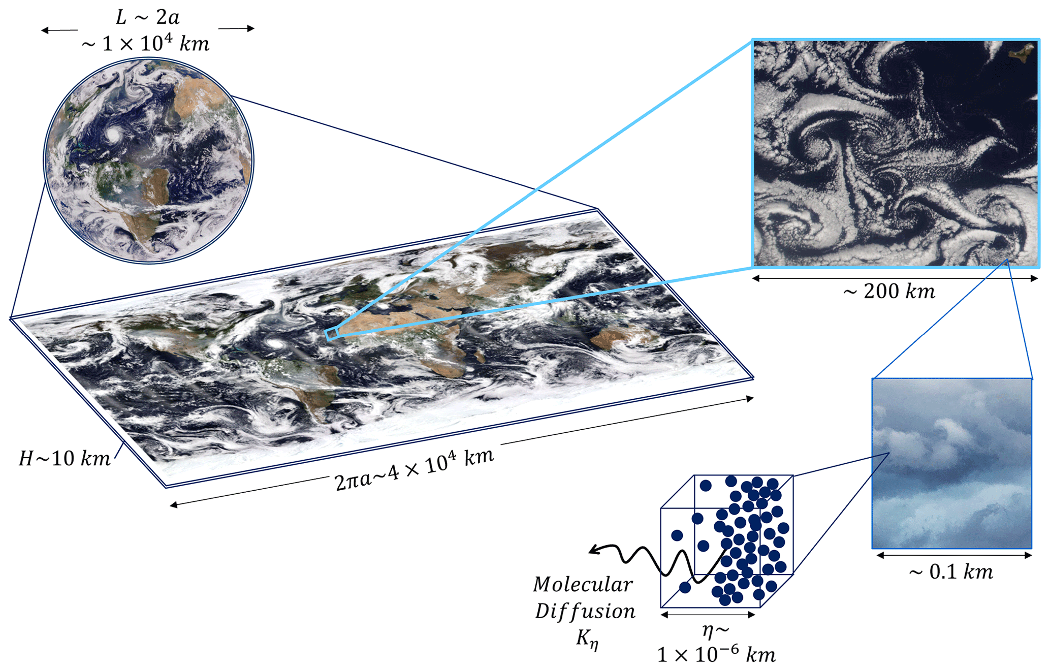
Figure 1 Diagram showing the similarity of rotational motions of clouds from the planetary diameter L∼2a, where structures are nearly 2D to smaller scales with more 3D structure. At L (left), swirling features associated with synoptic-scale systems are ∼10⁴ km long and nearly 2D compared to the tropospheric depth, H. At smaller resolved scales, the vertical component is more similar to the horizontal component, and thus the structure is more 3D. The images on the left are from EPIC (top) and a MODIS and VIIRS composite (bottom) for the same time frame. The upper-right inset shows cloud features shaped by von Kármán vortices viewed near the Canary Islands obtained by VIIRS with eddy length scales of ∼10 km. The image on the bottom-right shows swirling clouds in a thunderstorm, photographed from the ground with a length scale of ∼0.01 km. The bottom inset is a cartoon depicting the smallest length scale of turbulence, the Kolmogorov microscale, η, where kinetic energy is dissipated to heat through molecular diffusion K_η, with individual cloud droplets illustrated as dots, with spacing to represent the cloud edge interface.

Specifically, Lovejoy et al. (2007) (hereafter L07), and, more comprehensively, Lovejoy and Schertzer (2013), provided evidence that, rather than two separate isotropic turbulence regimes, the atmosphere is best characterized by a single anisotropic turbulence regime spanning all scales in the atmosphere. Following the framework of generalized scale invariance (GSI), which accounts for stratification, the “23/9D” elliptical model of turbulence in the atmosphere is characterized by a dimension that is intermediate to 2D and 3D (Schertzer and Lovejoy, 1985). Power spectra of radar reflectivity, cloud radiance, wind speed, and temperature all revealed length-scaling exponents that lie between purely 2D and 3D turbulence cases, which is consistent with an anisotropic turbulence regime predicted to have a volume dimension of $D=\mathrm{2.55}=\mathrm{2}+{\mathcal{H}}_z$, where ℋ_z≈0.55 is the ratio of horizontal and vertical values of ℋ (discussed further in Sect. 5) (Schertzer and Lovejoy, 1985; Lovejoy and Schertzer, 1985; Lovejoy et al., 1993; Lovejoy, 2021). For the Gaussian case, which does not include intermittency or multifractal aspects, ℋ is calculated from the power spectrum of the observed phenomenon, $E\left(k\right)\sim k^{-B}$, where $B=\mathrm{2}\mathcal{H}+\mathrm{1}$. In the 23/9D theory, which incorporates the vertical and horizontal aspects of separation, ${\mathcal{H}}_z=(B_{\mathrm{V}}-\mathrm{1})/(B_{\mathrm{H}}-\mathrm{1})$.

Simplifications of the first-order structure function have also been used to determine ℋ for properties of clouds (Pressel and Collins, 2012; Pressel et al., 2014) and to link the dimension of turbulence to the fractal dimension through the expression (Hentschel and Procaccia, 1984; Mandelbrot, 1985)

$$\begin{array}{}\text{(4)}& D=\mathrm{2}-\mathcal{H}.\end{array}$$

Equation (4) is the 2D analog of the fractal dimension of a geometric set of points. For example, given (x,Θ(x)), where x is the position in a 1D transect and Θ is the measured cloud brightness, the 1D case $D=\mathrm{1}-\mathcal{H}$ extends to the 2D cloud perimeter (Θ(x,y) as $D=\mathrm{2}-\mathcal{H}$ (Hentschel and Procaccia, 1984).

Observations of scaling behaviors in clouds, expressed through either the fractal dimension or the turbulent structure functions, point to a robust relationship between ξ, cloud geometry, and turbulence. This paper explores the topic as follows. In Sect. 2, we relate the Hurst exponent to an “ensemble” fractal dimension D_e that defines a globally distributed cloud field and discuss in Sect. 3 a resolution-coarsening procedure to measure it. Section 4 presents the values of the ensemble fractal dimension obtained using several satellite and numerical model datasets. Section 5 interprets the significance of the results by comparing them to the expected values of D_e and ℋ for 2D and 3D isotropic turbulence as well as for an anisotropic turbulence regime that is intermediate to 2D and 3D at all scales. Our findings contradict the theories proposing split 2D and 3D isotropic turbulence regimes separated by a scale break that have prevailed over the past few decades (Fiedler and Panofsky, 1970; Nastrom et al., 1984) and support the concept of a wide-ranging, scale-invariant 2D–3D anisotropic turbulence regime proposed by Schertzer and Lovejoy (1985), described in detail by Lovejoy and Schertzer (2013). We show that this anisotropic turbulence regime applies to cloud perimeters over a remarkable 10 orders of magnitude, ranging from the Kolmogorov microscale, η, to the planetary diameter, 2a.

2 Analytical expressions relating the perimeter of cloud ensembles to the dimension of turbulence

To explore how the cloud perimeter varies with measurement resolution ξ, the total perimeter of a cloud ensemble viewed from above (e.g., looking down as a satellite would view it from space) can be expressed in terms of a “perimeter density”. The perimeter density, 𝒫, is defined as the summed perimeters p of all clouds $P=\sum p$ normalized by the area of the horizontal domain, A_d; that is, $\mathcal{P}=P/A_{\mathrm{d}}$, a quantity analogous to the cloud fraction $\mathcal{A}=A/A_{\mathrm{d}}$, where A is the total cloud area. In this section, we show how 𝒫 can be related to ξ through the Hurst exponent, ℋ.

2.1 Cloud perimeter and the Hurst exponent

In Garrett et al. (2018), the total cloud edge perimeter, P, of a tropical convective cloud field was estimated theoretically for equal horizontal and vertical resolutions ${\mathit{\xi }}_{\mathrm{H}}={\mathit{\xi }}_{\mathrm{V}}=\mathit{\xi }$ within a domain volume V=A_dξ_V. To obtain P, a “mixing engine” framework was introduced that described cloud edge circulations consisting of coupled large-scale vertical buoyancy oscillations and horizontal turbulent exchanges as shown in Fig. 2. The derivation reflects a dimensional balance between two speeds. In the horizontal, v_H=K𝒫 represents a speed of erosion or formation of cloud edge due to dissipative mixing with a characteristic length scale ξ_H. The speed in the vertical direction is v_V=𝒩ξ_V, where 𝒩 is the moist adiabatic Brunt–Väisälä frequency, and represents the speed of production of potential energy through oscillatory vertical motions. Assuming a steady state and that the speeds of the horizontal and vertical legs of the circulation are equal, i.e., v_V=v_H, then it follows that

$$\begin{array}{}\text{(5)}& K\mathcal{P}=\mathcal{N}{\mathit{\xi }}_{\mathrm{V}}\end{array}$$

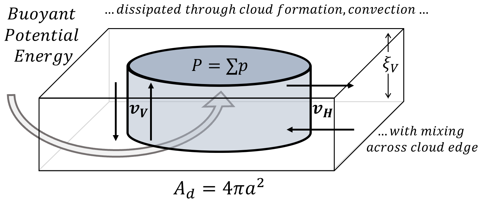
Figure 2 Illustration of the theorized cloud edge mixing engine from Garrett et al. (2018). The circulations are generated from the production and dissipation of buoyant potential energy at the planetary scale. All clouds in the domain area A_d of Earth's surface are represented as a single cylinder with a total perimeter of $P=\sum p$. The total available buoyant potential energy is dissipated vertically through moist adiabatic convection with vertical buoyancy speed v_V∼𝒩ξ_V and horizontally via turbulent mixing at the cloud edge with a speed of v_H∼K𝒫. Globally, the vertical and horizontal components must be in balance.

After invoking mass continuity for the cloud edge circulation, $\mathrm{\nabla }\cdot \mathit{v}=\mathrm{0}$ leads to $\partial v_{\mathrm{V}}/\partial {\mathit{\xi }}_{\mathrm{V}}=-\partial v_{\mathrm{H}}/\partial {\mathit{\xi }}_{\mathrm{H}}$, and through scale analysis, $\mathcal{N}{\mathit{\xi }}_{\mathrm{V}}/{\mathit{\xi }}_{\mathrm{V}}\sim K\mathcal{P}/{\mathit{\xi }}_{\mathrm{H}}$. Thus, if ξ_H is the horizontal measurement resolution ξ viewed from space, the following applies:

$$\begin{array}{}\text{(6)}& {\mathcal{P}}_{\mathit{\xi }}\sim {\displaystyle \frac{\mathcal{N}\mathit{\xi }}{K_{\mathit{\xi }}}},\end{array}$$

where K_ξ is the turbulent eddy diffusivity with eddy length scale, ξ.

From Eq. (3), we see that K_ξ scales with ℋ, the value of which varies depending on the dimensionality of turbulence reflecting any anisotropy between ξ_V and ξ_H. The adjustment needed to scale K_ξ from the molecular diffusivity at η (i.e., K_η, the diffusion coefficient of air) to the resolution ξ is (Richardson, 1926; Garrett et al., 2018)²

$$\begin{array}{}\text{(7)}& K_{\mathit{\xi }}=K_{\mathit{\eta }}{\left({\displaystyle \frac{\mathit{\xi }}{\mathit{\eta }}}\right)}^{\mathrm{1}+\mathcal{H}}.\end{array}$$

After substituting Eq. (7) into Eq. (6), the expected relationship relating the measurement resolution to the cloud perimeter density 𝒫_ξ becomes

$$\begin{array}{}\text{(8)}& {\mathcal{P}}_{\mathit{\xi }}={\displaystyle \frac{\mathcal{N}\mathit{\eta }}{K_{\mathit{\eta }}}}{\left({\displaystyle \frac{\mathit{\eta }}{\mathit{\xi }}}\right)}^{\mathcal{H}}\propto {\mathit{\xi }}^{-\mathcal{H}}.\end{array}$$

An observed value of ℋ is then obtainable from measurements of 𝒫 as a function of ξ.

2.2 The fractal dimension of cloud ensembles

Equation (8) expresses the cloud perimeter as a function of resolution and is thus analogous to Eq. (1), where $p\propto {\mathit{\xi }}^{\mathrm{1}-D}$ with fractal dimension D. The canonical value for individual clouds is $D\approx \mathrm{4}/\mathrm{3}$ (Lovejoy, 1982; Siebesma and Jonker, 2000; Christensen and Driver, 2021), but there are complications with this expression for D, including the aforementioned multifractal nature of clouds. Additionally, D in the expression $p\propto {\sqrt{a}}^D$ mathematically only applies to the shape of an individual cloud and has been argued to only represent sets of identically shaped objects (Imre, 1992).

From a climatological perspective, it is instead the ensemble of clouds with total perimeter density 𝒫 that governs exchanges of energy and air across cloud edges. Following the fractal “islands” analogy from Mandelbrot (1977), who considered the total perimeter of an ensemble of objects (described in more detail below), we propose an “ensemble fractal dimension” for clouds D_e that is analogous to Eq. (1) such that

$$\begin{array}{}\text{(9)}& {\mathcal{P}}_{\mathit{\xi }}\propto {\mathit{\xi }}^{\mathrm{1}-D_e},\end{array}$$

implying from Eq. (6) that the scaling exponent of the diffusivity is equivalent to the ensemble fractal dimension:

$$\begin{array}{}\text{(10)}& K_{\mathit{\xi }}\propto {\mathit{\xi }}^{D_e}.\end{array}$$

The distinction between D and D_e was first raised by Mandelbrot (1977), who showed that an ensemble of fractal islands with power-law distributed areas a follows the Korčák law, that is a survival function, $S(a^{\prime }>a)\propto a^{-\mathcal{K}}$ (Korčák, 1938), where the ensemble fractal dimension of the total coastline perimeter P is D_e=2𝒦, confined to the bounds $\mathrm{1}\le D<D_e\le \mathrm{2}$.

The survival function can be related to a cumulative distribution function (CDF) through $S=\mathrm{1}-\text{CDF}$, and 𝒦 is equivalent to the exponent of the power-law number distribution (Clauset et al., 2009). The area number distribution can be expressed as $n_a\propto a^{-(\mathrm{1}+\mathit{\alpha })}$ for clouds (Cahalan and Joseph, 1989; Benner and Curry, 1998; Wood and Field, 2011) and 𝒦∼α. The perimeter number distribution, $n_p\propto p^{-(\mathrm{1}+\mathit{\beta })}$, is related to that for the area through $\mathit{\alpha }=D\mathit{\beta }/\mathrm{2}$ for clouds (DeWitt et al., 2024). It follows that the ensemble fractal dimension is given by D_e=Dβ. The inequality D<D_e requires that β>1.

Comparing the exponents in Eqs. (8) and (9), the Hurst exponent can be related to the ensemble fractal dimension through

$$\begin{array}{}\text{(11)}& \mathcal{H}=D_e-\mathrm{1}.\end{array}$$

This equation is important because it provides a means for linking satellite observations of cloud perimeter fractal properties and size distributions to the less easily seen but more physically relevant turbulent structures at the cloud edge. For comparison with a large eddy simulation (LES) model of a tropical cloud field resolved at 100 m scales, Garrett et al. (2018) applied a value of $\mathcal{H}=\mathrm{1}/\mathrm{3}$ to Eq. (7) consistent with Richardson (1926) and the $\mathrm{4}/\mathrm{3}$ law. What is implicit in this case is an assumption of 3D isotropic turbulence at resolved scales. The assumption may be appropriate for an LES that chooses a cubic Eulerian grid for computational ease at the expense of losing a Lagrangian perspective.

However, while $D=\mathrm{4}/\mathrm{3}$ is consistent with values seen for individual clouds, a larger value is required for cloud ensembles, in which case the inequality D<D_e predicted by Mandelbrot (1977) and DeWitt et al. (2024) applies. In a similar adjustment to the individual fractal dimension, Hentschel and Procaccia (1984) related the perimeter fractal dimension of clouds to ℋ through the expression $D=\mathrm{2}-\mathcal{H}$ (Eq. 4), with a correction for turbulent intermittency (μ, where $D_{\mathit{\mu }}=(\mathrm{4}+\mathit{\mu })/\mathrm{3}\approx \mathrm{5}/\mathrm{3}$ (described below). We obtain, from Eqs. (11) and (4), an adjustment to D for an ensemble of clouds:

$$\begin{array}{}\text{(12)}& D_e=\mathrm{3}-D.\end{array}$$

The quantity 3−D has been defined as the intermittency exponent by Hentschel and Procaccia (1984) and the multifractal codimension³ (Schertzer and Lovejoy, 1987) within a 3D space. Applying the canonical value of $D=\mathrm{4}/\mathrm{3}$ for individual clouds leads to the expected value of $D_e=\mathrm{5}/\mathrm{3}$ for cloud ensembles. Perhaps the geometric intermittency of multiple and varied cloud types in an ensemble reflects the turbulent intermittency that is not represented by D for individual clouds. This estimate of $D_e=\mathrm{5}/\mathrm{3}$ is in agreement with Hentschel and Procaccia (1984), who found that Richardson's $\mathrm{4}/\mathrm{3}$ law only applies if the fractal dimension is $D_{\mathit{\mu }}=\mathrm{5}/\mathrm{3}$, obtained by adding an intermittency correction with a value of $\mathrm{0.25}<\mathit{\mu }<\mathrm{0.5}$ to the value $D=\mathrm{4}/\mathrm{3}$. The $\mathrm{5}/\mathrm{3}$ value is also nearly identical to the value of $D_e=\mathrm{1.68}\pm \mathrm{0.06}$ obtained from D_e=Dβ for β=1.26 from DeWitt et al. (2024), which applied across various satellite instruments and climate regimes. In this case, the implied value of the Hurst exponent is $\mathcal{H}=\mathrm{2}/\mathrm{3}$, which is between the 3D turbulence value of $\mathcal{H}=\mathrm{1}/\mathrm{3}$ and the 2D turbulence value of ℋ=1. Using Eq. (9) and the methods below, we observationally evaluate the applicability of the result $\mathcal{H}=\mathrm{2}/\mathrm{3}$ that is associated with $D_e=\mathrm{5}/\mathrm{3}$.

Mandelbrot (1967)Kolmogorov (1941)Richardson (1926)Kolmogorov (1941)Hentschel and Procaccia (1984)Garrett et al. (2018)Krueger et al. (1997)Mandelbrot (1977)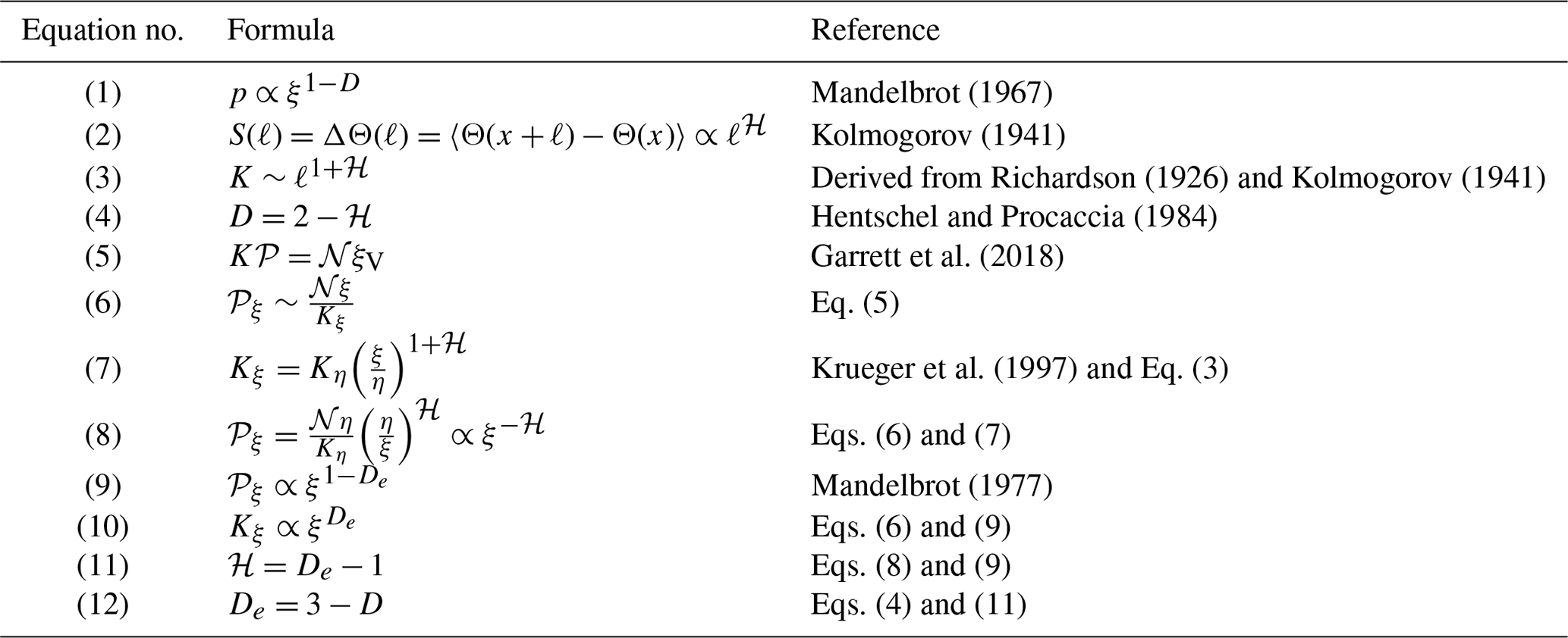

Table 1 Summary of main formulas.

3 Data and methods

Equation (11) implies that the dimensionality of the turbulent structure in clouds can be inferred from observations of cloud perimeters. To explore this hypothesis and the suggestion from Eq. (12) that $\mathcal{H}=\mathrm{2}/\mathrm{3}$, we consider satellite imagery of clouds from platforms in polar-orbiting, geostationary, and heliocentric orbits (summarized in Table 2) using cloud mask algorithms. The resulting binary arrays, hereafter “cloud masks”, represent cloudy pixels with a value of unity and clear skies by a value of zero. Cloudy pixels are considered an individual connected cloud when they are vertically or horizontally adjacent (i.e., “four-connectivity”). The edges of the domain are not included as part of the perimeter. The quantities p and a are calculated for all individual clouds (see Fig. 3f for an example). The perimeter is defined as the sum of all pixel edge lengths along the outer edge of each cloud. Although the example shows that all pixel sizes are equal, in satellite imagery, each pixel has individual values of ξ_x and ξ_y for its width and height, which are adjusted from ξ_N to account for the Earth's curvature away from the satellite nadir vertically and horizontally. The area is the sum of ξ_x×ξ_y for each pixel in the cloud. For each image, p and a are summed and normalized by domain area A_d to determine 𝒫 and 𝒜.

The polar-orbiting datasets considered are from the instruments VIIRS and MODIS, which have native pixel resolution ξ_N at the nadir of 0.75 and 1 km and capture imagery in narrow, meridional swaths. Values of ξ_N represent the pixel resolution at satellite nadir; the horizontal and vertical dimensions of each pixel are adjusted based on their distance from the nadir. The average swath size for VIIRS is 2501 × 12 944 pixels with a domain area A_d of 2.6×10⁷ km². For MODIS, it is 1261 × 8120 pixels with $A_{\mathrm{d}}=\mathrm{2.0}\times {\mathrm{10}}^{\mathrm{7}}$ km². The VIIRS and MODIS datasets include 60 and 72 cloud masks from 2 June 2021. Their respective cloud mask techniques are described by Kopp et al. (2014) and Ackerman et al. (2008). We also include 12 MODIS cloud masks with 0.25 km resolution as defined by optical reflectance values R≥0.01 described by DeWitt et al. (2024). These high-resolution cloud masks have $A_{\mathrm{d}}=\mathrm{5.1}\times {\mathrm{10}}^{\mathrm{6}}$ km² and average image dimensions of 5048 × 8120 pixels obtained from 1 through 9 January 2021.

Geostationary datasets are obtained from instruments denoted here by their more familiar satellite names, Himawari (instrument name: AHI), GOES-West (ABI), and Meteosat-11 (SEVIRI), which provide full-disk imagery of Earth with $A_{\mathrm{d}}=\mathrm{1.0}\times {\mathrm{10}}^{\mathrm{8}}{\mathrm{km}}^{\mathrm{2}}$ positioned over the fixed longitudes 141° E, 137° W, and 0°, respectively. Their nadir pixel resolutions are 2, 2, and 3 km, respectively, with cloud masks as described by Derrien and Gléau (2005). For each of the geostationary datasets, 30 cloud masks were obtained from 2 June through 1 July 2021, each at approximately the local noon at the satellite nadir.

To provide unique observations of global cloud coverage, we also include cloud masks from GEO-Ring and EPIC. GEO-Ring is a composite of geostationary satellite imagery (Ceamanos et al., 2021) that provides stitched satellite imagery of the surface of the Earth (excluding the poles), with $A_{\mathrm{d}}=\mathrm{4.4}\times {\mathrm{10}}^{\mathrm{8}}$ km² at ξ_N=11 km. In total, 39 GEO-Ring cloud masks were obtained from 2 through 21 June 2021. EPIC obtains full-disk imagery of Earth from the DSCOVR satellite in heliocentric orbit, photographing Earth as it rotates and providing coverage of all longitudes. Due to its location at the L1 Lagrange point in deep space, EPIC imagery has a coarser pixel resolution of 8 km. In total, 30 EPIC cloud masks (described by described by Yang et al., 2019) were obtained from 1 through 30 June 2017.

DeWitt et al. (2024)Kopp et al. (2014)Ackerman et al. (1998, 2008)Derrien and Gléau (2005, 2010)Derrien and Gléau (2005, 2010)Derrien and Gléau (2005, 2010)Yang et al. (2019)Ceamanos et al. (2021)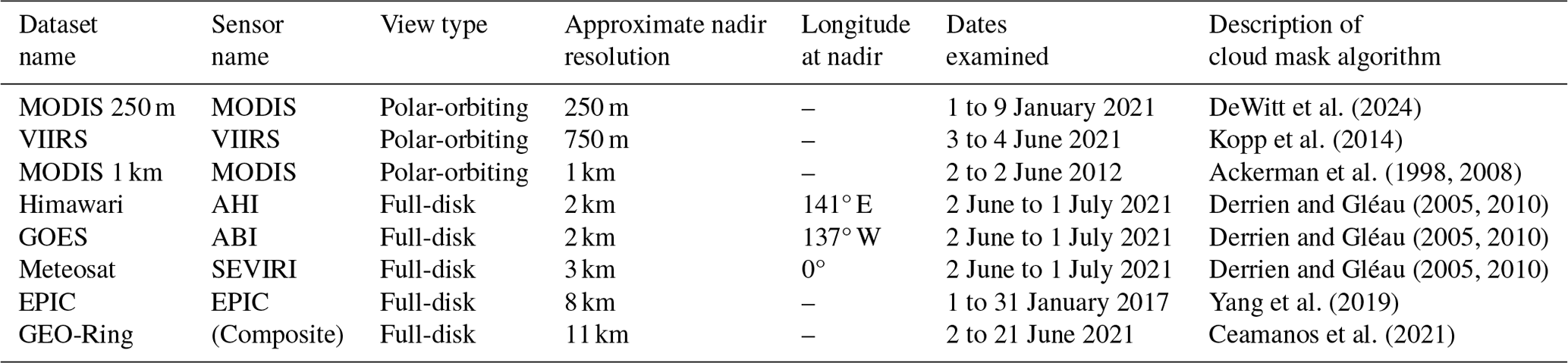

Table 2 Summary of satellite datasets used in this study.

As a means to compare measurements of 𝒫_ξ from satellite observations to the value derived by Garrett et al. (2018), we consider the geometries of clouds simulated using the System for Atmospheric Modeling (SAM), calculated as they would be viewed from space. SAM is a high-resolution 3D LES, initialized with idealized GATE phase III campaign soundings for tropical convection. The simulation domain of 204.8 km × 204.8 km × 19 km includes more than 1 billion grid points – often referred to as a “Giga-LES”. There are 2048 grid points in the horizontal directions with a grid spacing of 100 m and 256 grid points in the vertical with grid spacing ranging from 50 to 100 m. The simulation is integrated at 2 s intervals for 24 h. Refer to Khairoutdinov et al. (2009) for a more complete description of the simulation. We analyze scenes hourly from hour 12 through hour 24 of the model to ensure that steady state has been reached.

In order to compare the 3D model data with 2D satellite retrievals, we define the SAM cloud masks as 3D binary arrays for mixing ratios of non-precipitating cloud condensate, q_n>0.01 g kg⁻¹. A 2D facsimile of a satellite cloud mask is created from a vertical projection of the 3D cloud mask that represents the view from above. The 2D binary cloud mask is assigned a cloudy pixel based on threshold value j, where the corresponding vertical columns of the 3D cloud mask have ${\sum }_{\mathrm{0}}^H$ (cloudy pixels) > j. For example, with a threshold value of j=3, each pixel in the 2D cloud mask is classified as cloudy if more than three of the pixels in the corresponding 3D vertical column are cloudy. Multiple 2D cloud masks were obtained using threshold values of j = 1, 2, 3, 5, 9, 15. This thresholding procedure is similar to an analysis performed by DeWitt et al. (2024) that compared differences in cloud statistics defined by various optical depth thresholds.

To obtain values of D_e, total cloud perimeter P is first calculated at the native spatial resolution, ξ_N, and normalized by A_d to obtain 𝒫_N. The image is then artificially coarsened (see description below), and the procedure is repeated. 𝒫_ξ is obtained at progressively coarser spatial resolutions ξ>ξ_N such that ξ=ξ_Nk, where k is the coarsening factor. Coarsening is performed by separating the original image into a grid of multiple “boxes” containing k×k pixels (see Fig. 3e, red boxes), which are reduced to a single upscaled pixel through averaging. Each pixel of the coarsened image (Fig. 3f, outlined in blue) is determined to be cloudy or clear by rounding the average of the values inside each box in the native-resolution image (Fig. 3e, outlined in blue) to unity or zero. The values of k are chosen to be the nearest odd integers that differ by a constant factor (e.g., k=2ⁿ). The maximum value of k for each dataset corresponds to coarsening to a single pixel along the shorter dimension of the domain. Figure 3a–d shows an example of resolution coarsening to a single pixel for various EPIC cloud masks.

A least-squares linear regression is performed on values of ln 𝒫_ξ and ln ξ to obtain the Hurst exponent ℋ and D_e from Eqs. (8) and (9). Linear regression was performed on the straightest region of all curves, which was found to be $\mathrm{7}<\mathit{\xi }/{\mathit{\xi }}_N<\mathrm{150}$, where biases due to interpolation ($\mathit{\xi }/{\mathit{\xi }}_N<\mathrm{7}$, most significantly for EPIC) and due to the square shape of pixels at very coarse resolutions ($\mathit{\xi }/{\mathit{\xi }}_N>\mathrm{150}$) are omitted. Uncertainties in the linear regression are evaluated at the 95 % confidence level.

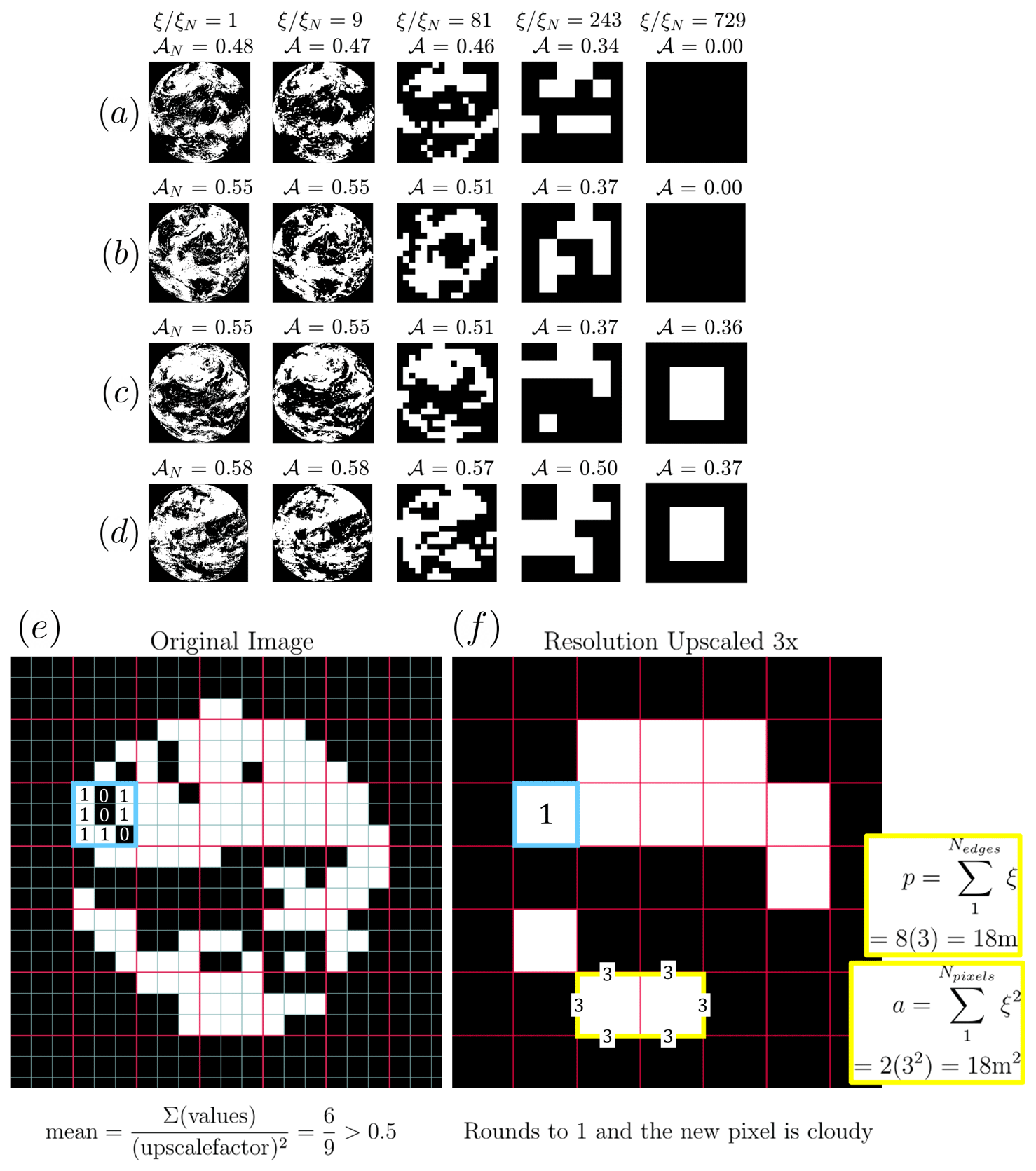
Figure 3 (a–d) EPIC cloud masks shown at native resolution, ξ_N, and coarsened resolution, ξ, down to a single pixel for four cases, with the initial native cloud fraction between $\mathrm{0.48}<{\mathcal{A}}_N<\mathrm{0.58}$ (increasing from top to bottom), illustrating a bifurcation of the cloud fraction, with the coarsening of the resolution depending on the native cloud fraction to either zero or unity. Note that the single pixel case shown here has a value of 𝒜=0.37 rather than unity because the domain area represented by the square pixel is the disk area A_d=πa². (e, f) A detailed example of the upscaling method. The “original” image here is shown at 100 times the resolution of the true original image to exaggerate pixels for clarity, and the coarsened image is upscaled 3 times or $k=\mathit{\xi }/{\mathit{\xi }}_N=\mathrm{3}$. The thin blue lines outline pixels with side-lengths ξ_N, and the red boxes are the upscaled pixel regions. An example region of pixels from which the mean is used to determine whether the upscaled pixel is cloudy or clear is highlighted as a thick blue box, with pixel values shown within. An example of the individual perimeter and area calculation is highlighted in yellow, assuming the original pixel resolution is ξ_N=1 m. Areas outside the circle are marked NaN and so are omitted from the average.

4 Results: cloud measurements

Alongside measurements of perimeter density, 𝒫_ξ, the more familiar quantity of cloud fraction, 𝒜_ξ, is included as a point of comparison. Figure 4 shows the cloud fraction and perimeter density obtained from satellite and model datasets at native resolution ξ_N, termed 𝒜_N and 𝒫_N, and coarsened resolution ξ normalized by ξ_N. Both ξ_N and domain area, A_d, span 2 orders of magnitude: ξ_N from 0.1 to 11 km and A_d from 5.1×10⁶ to 4.4×10⁸ km².

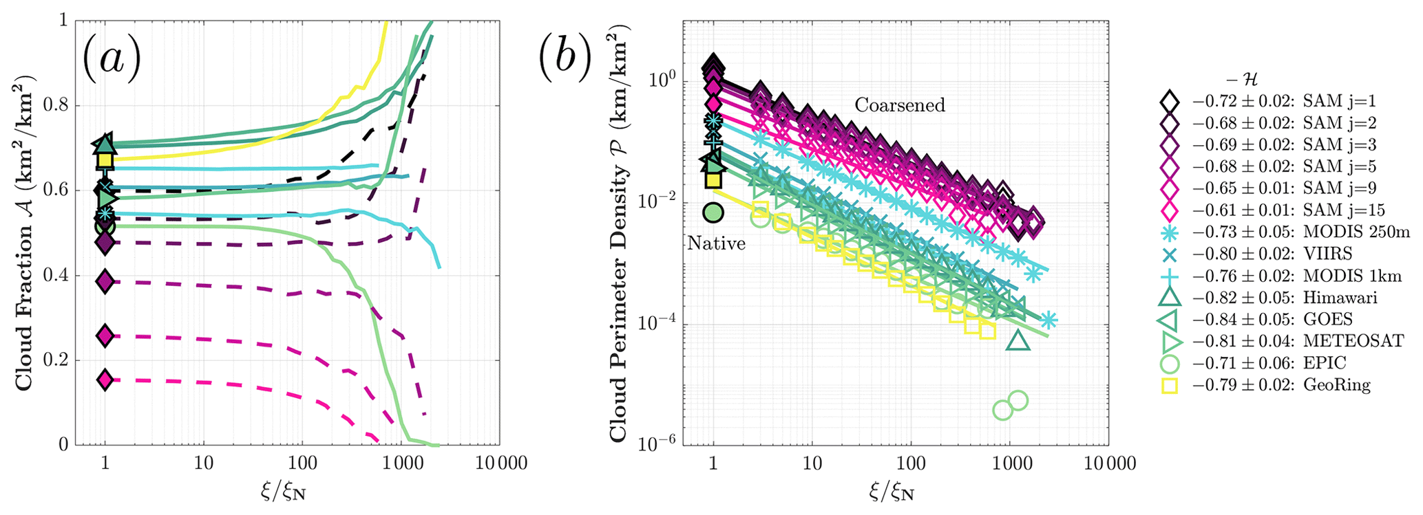
Figure 4 Measured cloud fraction, 𝒜_N (a), and perimeter density, 𝒫_N (b), at native measurement resolution, ξ_N (solid markers), and 𝒜_ξ and 𝒫_ξ at coarsened resolution, ξ, normalized by ξ_N (lines and hollow markers) for polar-orbiting (blue), full-disk (green), and global mosaic (yellow) satellite datasets. The SAM numerical simulations are shown as pink diamonds (with brightness scaled by threshold value j). Legend entries are sorted by increasing ξ_N with the associated negative Hurst exponent, ℋ, obtained from a least-squares linear regression of ln 𝒫_ξ and ln ξ (Eq. 8) and uncertainties evaluated for a 95 % confidence interval. Linear regression was performed on the straightest portion of all curves and found to be $\mathrm{7}<\mathit{\xi }/{\mathit{\xi }}_N<\mathrm{150}$ although the best-fit lines are extrapolated to all points to show their relative distance to the fit.

4.1 Measured cloud fraction, 𝒜

Global cloud fraction values, 𝒜_N, in Fig. 4a range from 0.5 to 0.7, reflecting differences in cloud mask techniques. With progressive coarsening, 𝒜 changes by less than 5 % before bifurcating at $\mathit{\xi }/{\mathit{\xi }}_N\sim \mathrm{100}$. As ξ approaches $\mathit{\xi }/{\mathit{\xi }}_N\sim \mathrm{1000}$, 𝒜 is represented by a single pixel, with a value of either zero or unity (except for the polar-orbiting satellites, which are represented by a 1 × 5 line). Interestingly, geostationary cloud fraction measurements with 𝒜_N>0.56 approach a value of unity, whereas MODIS 0.25 km and EPIC datasets with 𝒜_N=0.55 instead trend toward zero.

This bifurcation of cloud fraction reflects that as an image of a cloud field is coarsened to a single pixel, the coarsened pixel value is determined by averaging and rounding to zero or unity the pixel values in the original image (illustrated in Sect. 3). Conversely, a coarsening method in which the presence of any cloudy pixels in the original image results in a cloudy coarsened pixel causes cloud fraction to converge to unity with coarsening (Di Girolamo and Davies, 1997). Due to this averaging method, the value to which cloud fraction bifurcates depends on the native cloud fraction, 𝒜_N. Figure 3 shows four examples of coarsening EPIC cloud masks to a single pixel, resulting in either a single clear or a cloudy pixel. Although statistically the initial cloud fraction value is a good indicator of whether the single pixel will be cloudy or clear, it is not the only factor. For 𝒜_N=0.55, the single-pixel value of 𝒜 depends more on the initial distribution of clouds. Where clouds are more evenly distributed across the globe (Fig. 3b), smaller isolated structures vanish more quickly with coarsening and approach 𝒜=0 for a single pixel. When clouds are more clustered (Fig. 3c), a coarsened single pixel has 𝒜=1.

The application of vertical pixel thresholding in SAM results in a wide range of native cloud fraction values of $\mathrm{0.15}<{\mathcal{A}}_N<\mathrm{0.60}$. Larger threshold values of j tend to exclude small and shallow clouds and, in turn, decrease the overall cloud fraction. Bifurcation of 𝒜 occurs for SAM at a native value of 𝒜_N≈0.45, which is notably smaller than the value at which bifurcation occurs for satellite datasets at 𝒜_N≈0.55. This discrepancy suggests a difference between the clustering behavior of clouds viewed globally by satellite and those of modeled clouds for a region of tropical convection. A possible explanation for the discrepancy is that models assume local thermodynamic equilibrium, which has been argued not to apply in the atmosphere (Tuck, 2022).

4.2 Measured cloud perimeter density, 𝒫

The resolution dependence of cloud perimeter density, 𝒫, can be defined more simply than for cloud fraction, 𝒜. As shown in Fig. 4b, perimeter density 𝒫_ξ has a power-law scaling with ξ in all datasets, independent of satellite orbit, domain size, and resolution. For ξ>ξ_N, 𝒫_ξ is well characterized by a linear regression of ln 𝒫_ξ to ln ξ (Eq. 8). Linear regression is performed only on data points in the straightest region of all curves, $\mathrm{7}<\mathit{\xi }/{\mathit{\xi }}_N<\mathrm{150}$, where biases due to interpolation ($\mathit{\xi }/{\mathit{\xi }}_N<\mathrm{7}$) and the square shape of pixels at very coarse resolutions ($\mathit{\xi }/{\mathit{\xi }}_N>\mathrm{150}$) are ignored. The lines in the figure are shown to be extrapolated to all points to demonstrate their relative distance to the least-squares fit, which can be assumed to more reliably reflect the physical fractal nature of the cloud ensemble. This power-law relationship ${\mathcal{P}}_{\mathit{\xi }}\propto {\mathit{\xi }}^{-\mathcal{H}}$ holds even past the point $\mathit{\xi }/{\mathit{\xi }}_N\sim \mathrm{100}$ where cloud fraction values of 𝒜 tend to diverge. However, for very large $\mathit{\xi }/{\mathit{\xi }}_N\sim \mathrm{1000}$, 𝒫_ξ can deviate from the power-law regression to lower values, reflecting the fractal nature of the problem: complex cloud structures cannot be fully represented by coarse Euclidean geometries such as a single square pixel. This low bias in 𝒫_ξ for values of $\mathit{\xi }/{\mathit{\xi }}_N$ between ∼100 and ∼1000 can also be seen in the fourth and fifth columns of Fig. 3a–d. There, for $\mathit{\xi }/{\mathit{\xi }}_N=\mathrm{243}$, the images appear pixelated but maintain their general structure. However, for $\mathit{\xi }/{\mathit{\xi }}_N=\mathrm{729}$, the cloud mask consists of either a single cloudy or a clear pixel. The value of $\mathit{\xi }/{\mathit{\xi }}_N$ at which 𝒫 begins to depart from the linear regression corresponds to the coarsest resolution for which the complexity of the cloud edge can still be reliably measured.

Notably, the value of 𝒫_N for the native resolution $\mathit{\xi }/{\mathit{\xi }}_N=\mathrm{1}$ does not always align with the best-fit line, especially for the case of EPIC. As discussed in DeWitt et al. (2024), EPIC employs an on-board averaging and post-processing interpolation that artificially smooths the edges of clouds to compress data for transmission. This interpolation results in the artifact that 𝒫_N is lowered due to the reduced edge complexity. A similar phenomenon is observed to a lesser degree for the other satellite datasets. To avoid this issue, the 𝒫_N data points are not included in the linear regression.

For satellite datasets, values of ℋ lie in the range $\mathrm{0.71}<\mathcal{H}<\mathrm{0.84}$, with a mean value of ℋ=0.78 and with uncertainty evaluated at the 95 % confidence interval of 0.09. The ensemble fractal dimension that corresponds to the total cloud perimeter given by Eq. (11) is $D_e=\mathcal{H}+\mathrm{1}=\mathrm{1.78}\pm \mathrm{0.09}$, which is larger than the canonical value of $D\approx \mathrm{4}/\mathrm{3}$ often observed for individual clouds obtained using the expression $p\propto {\sqrt{a}}^D$. Calculated values of ℋ from the satellite datasets do not appear to depend on the type of satellite orbit or resolution, but they are significantly larger than those found for modeled clouds. 𝒫_ξ measured from SAM follows a power law, with exponent values in the range $\mathrm{0.60}<\mathcal{H}<\mathrm{0.71}$ depending on threshold value, j. The average value of $\mathcal{H}=\mathrm{0.67}\pm \mathrm{0.08}$ is 2 standard deviations smaller than the satellite datasets.

Note that modeled values of ℋ lie closer to the value of $\mathrm{1}/\mathrm{3}$ expected for 3D isotropic turbulence than inferred from the satellite datasets, perhaps reflecting the smaller domain area and atmospheric regime or assumptions used in LES models of subgrid-scale turbulence or local thermodynamic equilibrium. In general, increasing the threshold value j (which determines the minimum vertical cloud thickness required for 2D cloud masking), leads to smaller values of ℋ, reflecting the multifractal nature of clouds. For example, for a detection threshold of j=0, all cloudy pixels in the domain are considered and ℋ=0.71. Meanwhile, for the highest detection threshold value of j=15, ℋ=0.61. The latter case requires that only the largest overlapping cloud structures are included in the analysis, leaving most small, shallow clouds omitted. The smallest clouds are only observed with the finest resolution, resulting in a shallower linear regression slope for more highly thresholded cloud scenes.

5 Discussion

To summarize the observations, global cloud perimeter density, 𝒫, is much more sensitive than cloud fraction, 𝒜, to the measurement resolution, ξ, but the dependence is also much more simply mathematically characterized. The observed power-law scaling relating 𝒫 to ξ is remarkably similar for imagery from a wide range of satellite platforms. We measured an ensemble fractal dimension of $D_e=\mathrm{1.78}\pm \mathrm{0.09}$, corresponding to a Hurst exponent of $\mathcal{H}=\mathrm{0.78}\pm \mathrm{0.09}$. Similarly, from DeWitt et al. (2024), $D_e=D\mathit{\beta }\simeq \mathrm{1.68}\pm \mathrm{0.06}$ is derived from satellite observations of the perimeter distribution power-law exponent $\mathit{\beta }=\mathrm{1.26}\pm \mathrm{0.06}$ and assuming $D=\mathrm{4}/\mathrm{3}$ for individual clouds.

To account for how the dimensionality of turbulence may help explain the difference between the measured value of $D_e=\mathrm{1.78}\pm \mathrm{0.09}$ for satellite observations (Fig. 4) and the theoretical value of $\mathrm{5}/\mathrm{3}$ implied by Eq. (12), we compare D_e with canonical values of ℋ associated with 2D, 3D, and “intermediate” turbulent regimes and explore limiting cases that correspond to possible upper and lower bounds of 𝒫_ξ evaluated at the planetary scale and the Kolmogorov microscale.

5.1 Scaling exponents for 3D, 2D, and intermediate turbulence regimes

As introduced in Sect. 1, the theory of 3D isotropic turbulence predicts that the length dependence of turbulent diffusivity follows $K\sim {\mathit{\epsilon }}^{\mathrm{1}/\mathrm{3}}{\mathrm{\ell }}^{\mathrm{4}/\mathrm{3}}$, i.e., Richardson's $\mathrm{4}/\mathrm{3}$ law. Within the context of resolved clouds, we express ℓ as the resolved eddy length ξ, assuming that the smallest resolved cloud features are shaped by turbulent eddies of that size. In this case, the turbulent diffusivity scaling expression for cloud edges resolved at scale ξ is

$$\begin{array}{}\text{(13)}& K_{\mathit{\xi },\mathrm{3}D}\propto {\mathit{\xi }}^{\mathrm{4}/\mathrm{3}}.\end{array}$$

Following from Eq. (3), $K\sim {\mathrm{\ell }}^{\mathrm{1}+\mathcal{H}}$ and the implied scaling exponent for velocity fluctuations in 3D isotropic turbulence is $\mathcal{H}=\mathrm{1}/\mathrm{3}$.

For 2D isotropic turbulence, where vertical motions are negligible due to, e.g., stratification, the diffusivity scaling exponent can be obtained from dimensional analysis with the conserved property being enstrophy ℰ – the integrated 2D vorticity squared – instead of ε. The dependence of ℰ on the eddy length scale, ℓ, is $\mathcal{E}\left(\mathrm{\ell }\right)\sim {\mathrm{\Phi }}^{\mathrm{2}/\mathrm{3}}{\mathrm{\ell }}^{\mathrm{3}}$, where Φ is the enstrophy flux density with units of s⁻³ (Kraichnan, 1967; Charney, 1971). The velocity scaling exponent is $v\sim {\mathrm{\Phi }}^{\mathrm{1}/\mathrm{3}}\mathrm{\ell }$, and after substituting v into K∼vℓ, the 2D turbulent diffusivity scaling becomes

$$\begin{array}{}\text{(14)}& K_{\mathit{\xi },\mathrm{2}D}\sim {\mathit{\xi }}^{\mathrm{2}}.\end{array}$$

Additionally, from Eq. (3), the implied scaling exponent for velocity fluctuations in 2D turbulence is ℋ=1.

The framework of generalized scale invariance (Schertzer and Lovejoy, 1985) allows for the derivation of an “elliptical dimension”, D_el, that applies to an “intermediate” 23/9D model of anisotropic turbulence at all scales in the atmosphere rather than distinct regions of 2D isotropic turbulence at large scales and 3D isotropic turbulence at smaller scales. This continuous scaling accounts for the horizontal–vertical anisotropy of the atmosphere due to stratification and is determined by comparing velocity fluctuations Δv_H and Δv_V corresponding to the horizontal velocity component, with subscripts H and V indicating the horizontal or vertical separation between measurements. Horizontal velocity fluctuations have been widely observed to follow a 3D scaling $\mathrm{\Delta }{v}_{\mathrm{H}}\sim {\mathit{\epsilon }}^{\mathrm{1}/\mathrm{3}}{\mathrm{\ell }}^{\mathrm{1}/\mathrm{3}}$, where ℓ ranges from the order of ∼1 m to the planetary scale (Lovejoy and Schertzer, 2013). The Bolgiano–Obukhov law (Bolgiano, 1959; Obukhov, 1959) describes the corresponding vertical scaling relationship in buoyancy-forced turbulence, $\mathrm{\Delta }{v}_{\mathrm{V}}\sim {\mathit{\varphi }}^{\mathrm{1}/\mathrm{5}}{\mathrm{\ell }}^{\mathrm{3}/\mathrm{5}}$, where ϕ is analogous to the potential energy dissipation rate ε in the vertical dimension, with units of m² s⁻⁵. To account for this anisotropy in the vertical, ℋ_z for the combined turbulence case was derived from the ratio of the horizontal and vertical Hurst exponents, ${\mathcal{H}}_{\mathrm{H}}=\mathrm{1}/\mathrm{3}$ and ${\mathcal{H}}_{\mathrm{V}}=\mathrm{3}/\mathrm{5}$, resulting in ${\mathcal{H}}_z={\mathcal{H}}_{\mathrm{H}}/{\mathcal{H}}_{\mathrm{V}}=\mathrm{5}/\mathrm{9}\sim \mathrm{0.56}$. From Eq. (11), the elliptical dimension becomes $D_{\mathrm{el}}=\mathrm{14}/\mathrm{9}=\mathrm{1.56}$ (for the volume, $\mathrm{23}/\mathrm{9}=\mathrm{14}/\mathrm{9}+\mathrm{1}$. See Lovejoy, 2023, for a review.) From Eq. (3), the turbulent diffusivity for this intermediate 23/9D regime then scales as follows:

$$\begin{array}{}\text{(15)}& K_{\mathit{\xi },\mathrm{int}}\sim {\mathit{\xi }}^{\mathrm{14}/\mathrm{9}}.\end{array}$$

Note that Eqs. (13) and (14) correspond to the isotropic cases of 2D and 3D turbulence, while Eq. (15) combines the vertical and horizontal components of ℋ to arrive at an anisotropic case of turbulent diffusivity expression that applies at all scales. Lovejoy et al. (2007) (L07) analyzed 5 m vertical resolution dropsonde wind datasets to determine the relationship $\mathrm{\Delta }{v}_{\mathrm{V}}\sim {\mathrm{\ell }}_{\mathrm{V}}^{{\mathcal{H}}_{\mathrm{V}}}$, where ℓ_V is the vertical separation between measurements. The observed Hurst exponent ranged from ℋ_V=0.60, in agreement with the Bolgiano–Obukhov $\mathrm{3}/\mathrm{5}$ scaling for ℓ_V<1 km, to ℋ=0.77 for ℓ_V<13 km, the tropospheric depth. Increasing values of ℋ_V as ℓ_V approaches the tropospheric depth were argued to be consistent with more 2D turbulent structures influenced by upper-level jet shear.

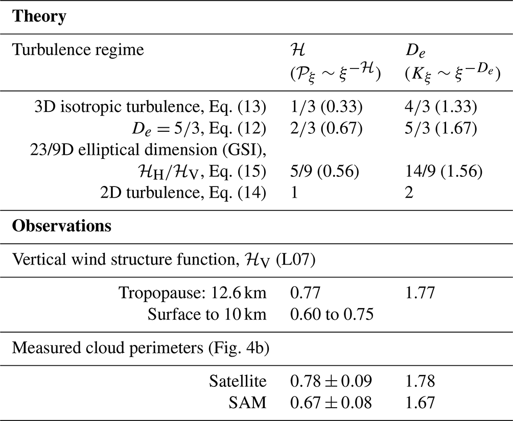
Table 3 summarizes previously derived expressions for the scaling exponents ℋ and D_e for 3D, 2D, and intermediate turbulence along with their relationship to 𝒫 through Eq. (8) for comparison with the satellite and numerical model results obtained here. The exponent values in Eqs. (13)–(15) are labeled D_e following Eq. (10).

Observational values from Sect. 4 and from L07 are similar to the theoretically obtained values of $D_e=\mathrm{5}/\mathrm{3}$ from Eq. (12) and the 23/9D model, implying $D_e=\mathrm{14}/\mathrm{9}=\mathrm{1.56}$, and not to either of the 2D or 3D isotropic turbulence. The $D_e=\mathrm{5}/\mathrm{3}$ case is closest to the value of $D_e=\mathrm{1.78}\pm \mathrm{0.09}$ obtained from satellite observations (Fig. 4b) and particularly to the range of values seen in SAM simulations ($\mathrm{1.61}<D_e<\mathrm{1.72}$).

Table 3 Theorized values (top) of ℋ and D_e from the expressions ${\mathcal{P}}_{\mathit{\xi }}\sim {\mathit{\xi }}^{-\mathcal{H}}$ (Eq. 8), $K_{\mathit{\xi }}\sim {\mathit{\xi }}^{D_e}$ (Eq. 10), and $\mathcal{H}=D_e-\mathrm{1}$ (Eq. 11) for the cases of 3D isotropic turbulence, $D_e=\mathrm{5}/\mathrm{3}$, the 23/9D elliptical model from generalized scale invariance (GSI), and 2D turbulence. Observations (bottom) include ℋ_V from Lovejoy et al. (2007) for vertical wind profiles and the measurements obtained here and shown in Fig. 4b. Values of ℋ for each case are compared in Fig. 6. Decimal values are shown alongside the derived fraction values for ease of comparison with observations.

5.2 Limiting cases: cloud perimeter density at the turbulent microscale and the planetary scale

Because cloud shapes and sizes are determined by objective physical processes that are independent of subjective measurement resolution, in principle it should be possible to infer information about cloud geometries from the physical properties of the planet and its atmosphere. To this end, we examine order-of-magnitude limiting case values for 𝒫 evaluated at the smallest and largest possible conceivable scales for clouds and expressed in terms of basic planetary and atmospheric parameters and compare these with the observations shown in Fig. 4b.

Given the turbulent nature of fractal cloud edges, the Kolmogorov microscale, η, is the smallest theoretical resolution length scale, ξ, for which 𝒫 is anticipated to be a maximum. Substituting ξ with η in Eq. (6) yields

$$\begin{array}{}\text{(16)}& {\mathcal{P}}_{\mathit{\eta }}={\displaystyle \frac{\mathcal{N}\mathit{\eta }}{K_{\mathit{\eta }}}}.\end{array}$$

For the planetary scale (denoted with ⊕), Eq. (5) becomes ${\mathcal{P}}_{\oplus }\sim \mathcal{N}H/K_{\oplus }$, where H is the atmospheric scale height. The planetary-scale diffusivity is $K_{\oplus }=LU$, where L=2a and U=𝒩H is the characteristic speed of the production and dissipation of moist convective potential energy in cloud edge circulations (described in Sect. 2). Thus, the following applies:

$$\begin{array}{}\text{(17)}& {\mathcal{P}}_{\oplus }\sim {\displaystyle \frac{\mathrm{1}}{\mathrm{2}a}}.\end{array}$$

This result is similar to the case where Earth is resolved as a single point source of light or a “pale blue dot” as coined by Sagan (1994). The extremely idealized case of perimeter density resolved by a single pixel is ${\mathcal{P}}_{\oplus }=P_{\oplus }/A_{\oplus }$. Considering either a square with a side-length ξ=2a ($\mathcal{P}=\mathrm{8}a/\left(\mathrm{4}{a}^{\mathrm{2}}\right)$) or a circular dot with diameter 2a ($\mathcal{P}=\mathrm{2}\mathit{\pi }a/\left(\mathit{\pi }{a}^{\mathrm{2}}\right)$) gives

$$\begin{array}{}\text{(18)}& {\mathcal{P}}_{\oplus ,\mathrm{PBD}}={\displaystyle \frac{\mathrm{2}}{a}}.\end{array}$$

In either case, 𝒫_⊕ is a function only of planetary radius a. Furthermore, each variable in Eq. (16) can be estimated from basic physical planetary properties, including the atmospheric composition, temperature, and pressure as described in Appendix A.

5.3 Comparison between observations and theory

Figure 5 presents observations and theoretical predictions of 𝒫_ξ. Theoretically derived estimates of 𝒫_ξ are obtained from Eq. (8) for three cases: 3D turbulence ($\mathcal{H}=\mathrm{1}/\mathrm{3}$ and $D_e=\mathrm{4}/\mathrm{3}$), 2D turbulence (ℋ=1 and D_e=2), and the intermediate case $D_e=\mathrm{5}/\mathrm{3}$. For clarity, the 23/9D case, which has a line nearly the same as the $D_e=\mathrm{5}/\mathrm{3}$ case, is not included in Fig. (5). Satellite and SAM measurements are clearly aligned with the case that $D_e=\mathrm{5}/\mathrm{3}$ as predicted by Eq. (12), lying distinctly between the curves corresponding to $D_e=\mathrm{4}/\mathrm{3}$ for 3D isotropic turbulence and D_e=2 for 2D turbulence. The limiting case for the Kolmogorov microscale, 𝒫_η, marks the intersection of 𝒫_ξ from Eq. (8), where ξ=η.

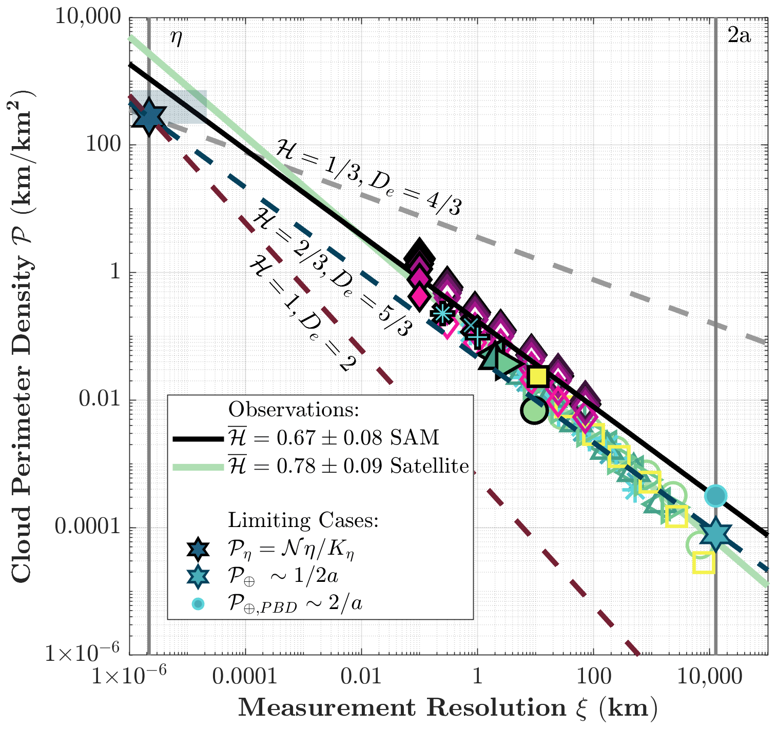
Figure 5 Measured perimeter density 𝒫_ξ for the satellites and SAM shown as the same markers from Fig. 4, with the derived 𝒫_ξ from Eq. (8) overlaid as gray ($\mathcal{H}=\mathrm{1}/\mathrm{3}$ and $D_e=\mathrm{4}/\mathrm{3}$ for 3D turbulence), blue ($D_e=\mathrm{5}/\mathrm{3}$), and red (ℋ=1 and D_e=2 for 2D turbulence) dashed lines. The average scaling exponents $\stackrel{\mathrm{‾}}{\mathcal{H}}$ are shown as solid green (satellite) and black (SAM) lines, with the mean and standard deviations in the legend. The limiting case value of 𝒫_η from Eq. (16) is shown as a dark-blue hexagram, with the uncertainty indicated by shading. The limiting case, 𝒫_⊕, at the planetary diameter ξ=2a from Eq. (17) is a light-blue hexagram, and the pale blue dot case from Eq. (18) is a light-blue circle.

What is striking is how well the predicted value of $D_e=\mathrm{5}/\mathrm{3}$ connects the highly idealized limiting case values of 𝒫_⊕ and 𝒫_η to the observed scaling for 𝒫_ξ. The alignment is particularly remarkable considering that 𝒫_η and 𝒫_⊕ are obtained only from the physical properties of the planet and its atmosphere and are separated by 10 orders of magnitude. This correspondence suggests that the statistical aspects of cloud geometries and atmospheric turbulence, D_e and ℋ, could in principle be inferred from knowing only a few basic physical parameters of a planet.

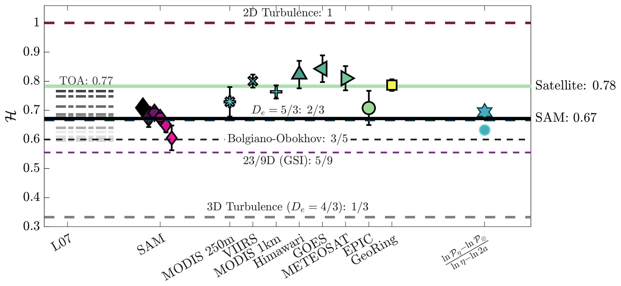
Figure 6 Visualization of theorized and observed ℋ. Theorized values of ℋ are shown as horizontal dashed lines for the 2D turbulence (red), $D_e=\mathrm{5}/\mathrm{3}$ (blue), Bolgiano–Obukhov scaling (black), 23/9D model from generalized scale invariance (GSI) (purple), and 3D turbulence (gray). Observations from Lovejoy et al. (2007) are shown (left) as horizontal dashed gray lines darkening as vertical separation distance ℓ_V increases from ℓ_V<158 m to ℓ_V=12.6 km, corresponding to the top of the atmosphere (TOA). Observations from this work (middle) are shown with symbols corresponding to Figs. 4b and 5, with the averages shown as horizontal green (satellite) and black (SAM) solid lines. On the right are markers corresponding to the slopes from 𝒫_η (Eq. 16) to the values of 𝒫_⊕ from Eqs. (17) and (18).

Figure 6 compares the observed and theoretical values of ℋ. The scaling relationship connecting microscale values (η,𝒫_η) to planetary values ($\mathrm{2}a,{\mathcal{P}}_{\oplus }$) and the scaling relationships inferred from observations lie between $\mathrm{1}/\mathrm{3}<\mathcal{H}<\mathrm{1}$, the limits for 3D and 2D turbulence. The values are the most consistent with the case $D_e=\mathrm{5}/\mathrm{3}$ and, to a lesser extent, with the 23/9D intermediate turbulence regime obtained from generalized scale invariance (Schertzer and Lovejoy, 1985; Lovejoy et al., 2007; Lovejoy and Schertzer, 2013) with $\mathcal{H}\sim \mathrm{5}/\mathrm{9}$.

Comparing the results here with observations of vertical wind structure functions by Lovejoy et al. (2007) (L07) in Fig. 6 and Table 3, values of ℋ for the smallest vertical separation distances in L07 (ℓ_V∼5 m, ℋ=0.60), and cloud structures resolved vertically in SAM (ξ_V∼100 m, ℋ=0.67) correspond most closely to the Bolgiano–Obukhov scaling, ℋ∼0.6. However, the value inferred from satellite observations (ℋ=0.78) is most consistent with L07 (ℋ_V=0.77) inferred from vertical separation distances of ℓ_V∼H. Despite these variations in ℋ, the observations of clouds reveal an intermediate turbulence regime that excludes both of the purely 2D or 3D isotropic turbulence cases.

5.4 Multifractal considerations

Because each of the satellite cloud masks considered in Fig. 4 is generated using a single respective cloud definition threshold, the above analysis is implicitly monofractal. Adopting a monofractal analysis of a field that is multifractal for such quantities as cloud brightness can be problematic. Most importantly, if the cloud brightness field were itself coarsened by averaging over adjacent pixels, the threshold applied to define the presence of a cloud would need to be adjusted to account for the inevitable smoothing of very bright regions with dark regions.

Here, this complication is limited because we are averaging adjacent pixels in a binary cloud mask rather than a brightness field, leading to a more accurate measurement of the fractal dimension (Lovejoy and Schertzer, 1991, Sect. A.4.ii) even as it still does not consider how the fractal dimension varies as a function of threshold. To address this question, we applied various values of the threshold parameter, j, to define cloudy pixels from the modeled cloud field in SAM. The parameter j is the number of cloudy pixels in each vertical column of the 3D volume required to assign a cloudy pixel in the horizontal 2D cloud mask. The vertical resolution of each pixel is 100 m in the vertical portion of the simulation domain that contains the most cloudy pixels. As shown in Fig. 4a, changing the threshold value of j results in a wide range of horizontal cloud fractions spanning $\mathrm{0.15}<\mathcal{A}<\mathrm{0.60}$. The multifractal nature of clouds is evident in Fig. 6: ℋ and D_e decrease by 0.11 as the threshold parameter, j, increases from 1 to 15. What remains clear is that, independent of the threshold considered, the central conclusion of this article remains unchanged, which is that measured values for ℋ are intermediate to those expected for 2D or 3D isotropic turbulence.

6 Conclusions

The measured relationship between the ensemble cloud perimeter density, 𝒫_ξ, seen from space and the resolution at which it is imaged, ξ, yields an ensemble fractal dimension, D_e, a scaling exponent analogous to the individual cloud fractal dimension D. We conclude that D_e represents the degree to which turbulence is 2D or 3D and simply corresponds to the Hurst exponent, ℋ, the basis of a scaling law for quantifying turbulent fluctuations in atmospheric scalars, through $D_e=\mathcal{H}+\mathrm{1}$.

Global cloud measurements of 𝒫 from various satellite orbit types and a large eddy simulation (LES) of tropical convection follow a consistent power-law scaling with respect to ξ across 5 orders of magnitude. The associated scaling exponent of $\mathcal{H}=\mathrm{0.78}\pm \mathrm{0.09}$ that we obtained from satellite measurements lies between the theoretical values for isotropic 2D and 3D turbulence, which is consistent with a model of anisotropic 23/9D turbulence (Schertzer and Lovejoy, 1985).

Measured values of the ensemble fractal dimension, D_e, are also greater than the value of $D\sim \mathrm{4}/\mathrm{3}$ that is often assumed to apply to individual clouds. The value obtained from SAM $D_e=\mathrm{1.67}\pm \mathrm{0.08}$ is equal to the theorized value of $D_e\sim \mathrm{5}/\mathrm{3}$ implied by Eq. (12). The measured value from satellite imagery $D_e=\mathrm{1.78}\pm \mathrm{0.09}$ is intermediate to the value of D_e=2 expected for 2D turbulence and $D_e=\mathrm{4}/\mathrm{3}$ for 3D turbulence. It is similar to a value of D_e=1.68 suggested by DeWitt et al. (2024) for cloud ensembles and to a theoretically derived value of $D_{\mathit{\mu }}\approx \mathrm{5}/\mathrm{3}$ obtained by Hentschel and Procaccia (1984) for intermittent turbulence. The value of D_e from satellite data is significantly greater than that obtained from the analysis of a detailed LES model of a tropical cloud field, suggesting that natural cloud ensembles are more geometrically complex.

Values of 𝒫 evaluated at the Kolmogorov microscale, η, and the planetary diameter, 2a, purely from physical parameters lie remarkably in line with satellite observations and LES model calculations despite being separated by 10 orders of magnitude in ξ. The value of 𝒫_η was only inferred from the molecular composition, temperature, and pressure of clouds and the atmosphere, while 𝒫_⊕ was inferred from the planetary radius, a; the atmospheric depth, H; and stability, 𝒩.

Globally distributed, the total perimeter of clouds has a resolution dependence in satellite and numerical datasets, one that can be tethered to physically parameterized values evaluated at the Kolmogorov microscale and the planetary diameter that points to the existence of an intermediate 2D/3D turbulence regime that applies at all conceivable tropospheric scales. Observations of clouds on other planets in the solar system could help identify whether the observed scaling is specific to present-day Earth or, in fact, general to stratified atmospheres. Any generalization of the scaling laws could prove useful for constraining predictions of cloud behaviors in a future climate state on Earth or for exoplanetary studies where – like Earth's pale blue dot – only coarse-resolution physical parameters are available.

Appendix A: Variables and parameters

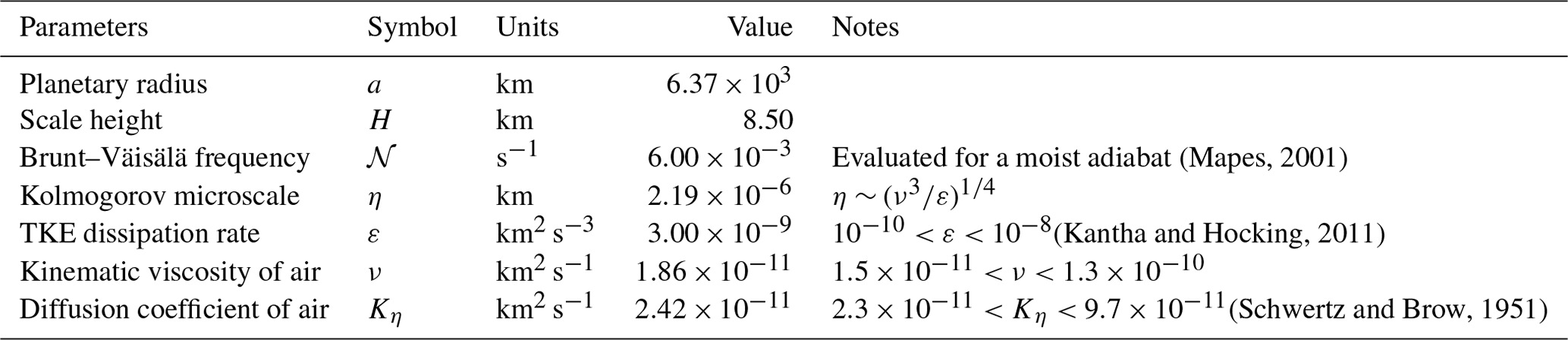
Values of the parameters and variables used for the calculation of 𝒫 in Eqs. (8) through (17) are shown in Table A1. Uncertainty in 𝒫_η and η owes to the range of possible values of ε, ν, and K_η. Diffusivity and kinematic viscosity are proportional to atmospheric pressure p, so uncertainties include the range of values corresponding to temperature T and p between the surface (T=300 K, p=1 bar) and the top of the troposphere (T=200 K, p=0.1 bar).

The Brunt–Väisälä frequency, 𝒩, for a dry adiabat is typically expressed as a function of gravity, g, and vertical temperature profiles but can also be expressed in terms of physical planetary parameters as $\mathcal{N}\sim g{\left(\frac{S(\mathrm{1}-\mathit{\alpha })}{\mathrm{4}\mathit{\sigma }}\right)}^{-\mathrm{1}/\mathrm{8}}{c}_p^{-\mathrm{1}/\mathrm{2}}$ (Read et al., 2016), where S is the solar constant, α is the planetary albedo, σ is the Boltzmann constant, and c_p is the specific heat at constant pressure. The value for a moist adiabat shown here is slightly less than but of the same order of magnitude as the value for a dry adiabat of 0.01 s⁻¹ (Mapes, 2001).

(Mapes, 2001)(Kantha and Hocking, 2011)(Schwertz and Brow, 1951)

Table A1 Values of variables and parameters described in the text used to determine theoretical values of 𝒫 shown in Fig. 5. TKE stands for turbulence kinetic energy.