Energy transfer from internal solitary waves to turbulence via high-frequency internal waves: seismic observations in the northern South China Sea

The shoaling and breaking of internal waves (IWs) are critical processes in the ocean's energy cascade and mixing. Using seismic data, we observed high-frequency internal waves (HIWs), which were primarily distributed in the depth range of 79–184 m. Their amplitude scale is O (10 m), with half-height widths ranging from 154 to 240 m. The shoaling thermocline and gentle slope with a low internal Iribarren number suggest that observed high-frequency internal waves are likely a result of fission. The remote sensing data support this point. Instability estimations showed that, due to the strong vertical shear, the Richardson number (Ri) in the range of 20–30 km was less than 0.25, and Kelvin–Helmholtz (KH) billows can be found in the seismic transect, suggesting that these waves were unstable and might dissipate rapidly. We used the seismic data to estimate diapycnal mixing, and we found that the HIWs can enhance diapycnal mixing, averaging 10⁻⁴ m² s⁻¹. The maximum mixing value is up to 10⁻³ m² s⁻¹, and it is associated with the breaking of IWs caused by the strong shear. The results show a new energy cascade route from shoaling internal solitary waves (ISWs) to turbulence, i.e., the fission of ISWs into HIWs, which improves our knowledge of ISW energy dissipation and their roles in improved mixing in the northern South China Sea.

1 Introduction

Internal solitary waves (ISWs) are widely distributed in the global ocean, and the South China Sea is recognized as one of the best places to study large-amplitude ISWs (Klymak et al., 2006; Zheng et al., 2022; Cai et al., 2015). After years of research, there is a clearer understanding of their generation, propagation, and evolution: barotropic tides interact with complex topography to produce internal tides (baroclinic tides), and internal tides radiate out from the Luzon Strait, with those radiating westward crossing the northern South China Sea basin and propagating towards slope and shelf areas. During propagation, nearly half of the internal tide energy generates ISWs through nonlinear steepening, and these waves deform due to shoaling effects, eventually breaking and dissipating on the shelf (Alford et al., 2015; Bourgault et al., 2007; Fu et al., 2012; Sinnett et al., 2022; Liu et al., 2022; Zhang et al., 2023). These large-amplitude ISWs have significant impacts on ocean mixing, sediment suspension, nutrient transport, and offshore oil and gas engineering (Bogucki et al., 1997; Osborne et al., 1978; Wang et al., 2007; Xu and Yin, 2011).

When energy is transferred from large and mesoscale motions to small-scale turbulence, internal waves (IWs) play a crucial role (Liu et al., 2022). Particularly in slope and shelf areas, the shoaling evolution and dissipation of IWs (primarily ISWs) are key processes driving turbulent mixing. As ISWs propagate from deep to shallow waters, they interact with the seabed topography, a process known as shoaling (Sinnett et al., 2022). Ocean instruments such as mooring and high-frequency acoustics can help us record this process better (e.g., Bourgault et al., 2007; Fu et al., 2012; Orr and Mignerey, 2003; Xu and Yin, 2012). Generally, at critical depths, the rear of a depression wave steepens and undergoes polarity reversal (the shape of the soliton evolves from depression to elevation as the slope of the leading edge is less than the trailing slope) to form an elevation wave (e.g., Shroyer et al., 2009). When the continental slope is relatively gentle, dispersion continues to form elevated wave trains, a process called fission (Bai et al., 2019; Djordjevic and Redekopp, 1978; Gong et al., 2021b; Liu et al., 1998; Zheng et al., 2001; Vlasenko and Hutter, 2002). In the slope and shelf regions of the South China Sea, where the topography is relatively gentle, ISWs frequently appear as wave packets through fission, as confirmed by satellite images (e.g., Zhao et al., 2003). During this process, the energy of ISWs continuously dissipates into the seawater, enhancing turbulent mixing. Studies have shown that the mixing caused by fission is second only to that caused by plunging breakers, which have a longer timescale for mixing over the length of the gentle slope (Masunaga et al., 2019). Ultimately, these shoaling waves break due to shear instability or convective instability, generating turbulence and achieving downscale transfer of ocean energy (Lamb, 2014). This represents our most common understanding of the dissipation mechanisms of ISWs.

However, Bai et al. (2013, 2019) discovered that ISWs on the South China Sea shelf also undergo fission to produce high-frequency internal waves (HIWs) during shoaling and proposed a new hypothesis for energy dissipation. They suggested that the fission of ISWs into HIWs is also a key process for energy dissipation. Their subsequent theoretical analyses and numerical simulations confirmed this hypothesis. In their review, Rippeth and Green (2020) pointed out that this finding is significant for understanding the dissipation mechanisms of ISWs. They think that the fission of ISWs into HIWs on the continental shelf is an important pathway for the tidal energy cascade.

Therefore, the energy dissipation mechanisms of IWs (ISWs) are complex, and the ocean is a multiscale coupled system with various dynamic processes. However, most current studies consider the ideal scenario where only IWs are present in the ocean's dynamic system, with few considering or only considering simplified dynamic environmental impacts. This results in an incomplete understanding of the shoaling processes and ISW dissipation mechanisms. Additionally, whether HIWs, another product of fission, significantly enhance energy dissipation and mixing remains a critical question for comprehending the formation and evolution of wave packets and their role in ocean mixing and energy cascades.

In this paper, we use the seismic method to investigate these questions. Seismic oceanography, initially proposed by Holbrook (2003), has provided us with a novel high-resolution method to image the thermohaline fine structure in the water column. The image formed by the reflection seismic method in the water column is mainly the result of the convolution of the seawater temperature gradient and the seismic source wavelet (Ruddick et al., 2009; Sallarès et al., 2009). Due to its advantages of fast acquisition, high horizontal resolution, and full-depth water column imaging, it has been widely proven to be an effective method for capturing ocean dynamic phenomena, covering a multiscale range from fine-scale O (10 m) to mesoscale O (100 km) (Song et al., 2021a). Many ocean features are captured and imaged through these high-resolution seismic images, such as ocean currents (e.g., Tsuji et al., 2005), eddies (e.g., Yang et al., 2022), fronts (e.g., Gunn et al., 2021), ISWs (e.g., Bai et al., 2017; Geng et al., 2019; Gong et al., 2021a; Song et al., 2021b; Tang et al., 2014, 2018), thermohaline staircases (e.g., Fer et al., 2010), and turbulence (e.g., Sheen et al., 2009). In recent years, this method has gradually become more quantitative, especially in estimating turbulent dissipation rates and diffusivity (e.g., Dickinson et al., 2017; Gong et al., 2021b; Tang et al., 2021; Yang et al., 2023). In this study, we applied this method to seismic line 25, where we sequentially observed HIWs generated by fission, bore-like nonlinear waves, and induced shear instabilities. Based on seismic data, we estimated turbulent dissipation rates and found that HIWs indeed enhance turbulent mixing. This indicates that the fission of ISWs into HIWs is also a key process for energy dissipation.

2 Data and methods

2.1 Seismic data acquisition and processing

From July to September 2009, the Guangzhou Marine Geological Survey Bureau conducted multichannel reflection seismic data collection on the northern slope and shelf of the South China Sea, covering 43 lines (not shown). Our study focused on seismic line 25 (the blue solid line in Fig. 1a), which was collected on 31 July. The acquisition vessel towed an air gun array with a total volume of 5080 in.³ (approximately 83 L) firing every 25 m (shot interval). The main frequency of the source was 35 Hz. A 6 km streamer with 480 hydrophones, spaced 12.5 m apart and with a minimum offset of 250 m (the distance from the air gun array to the nearest hydrophone), was towed to receive reflections, sampling every 2 ms.

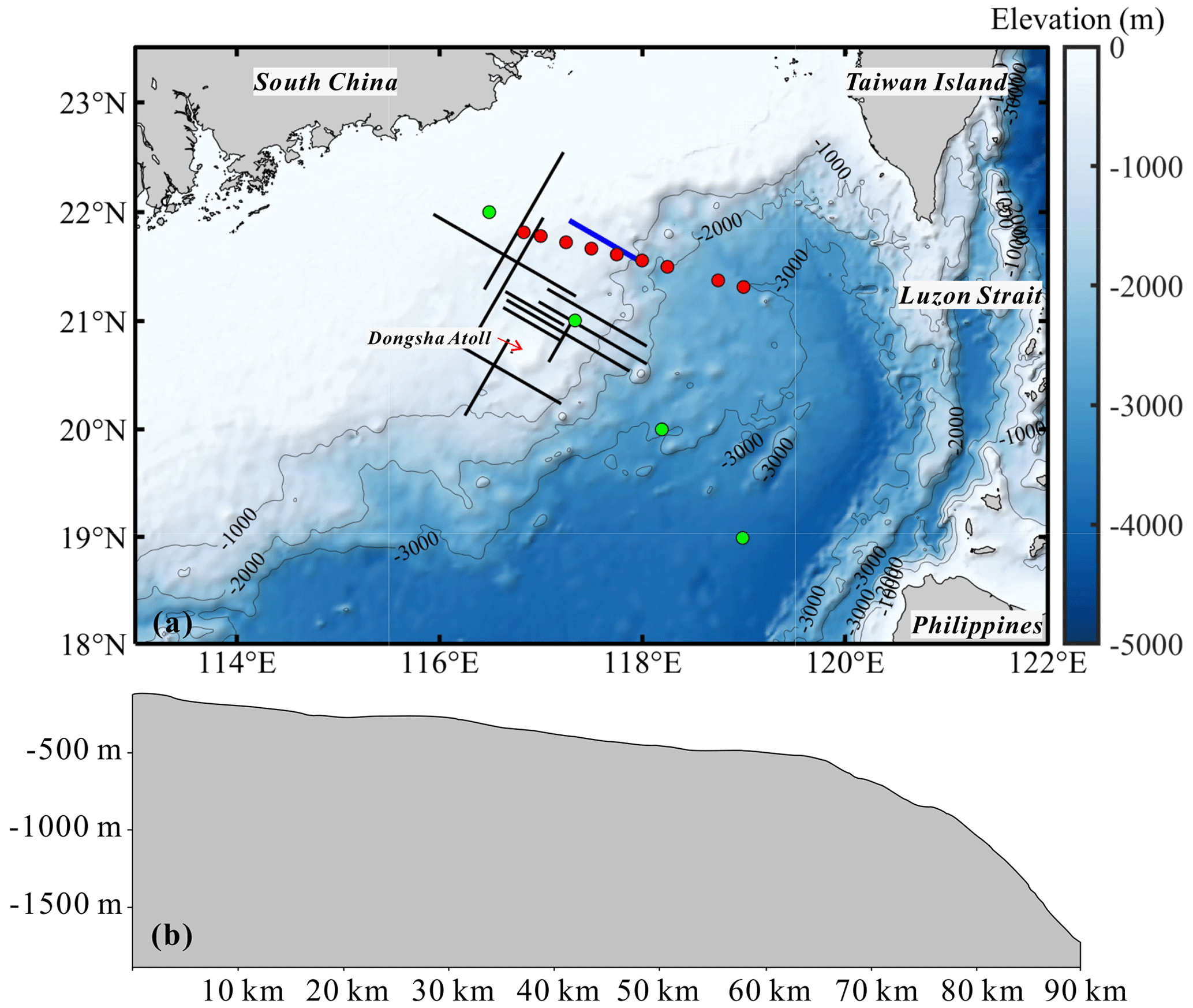
Figure 1 Bathymetry map of the South China Sea and seabed topography along seismic line 25. (a) Topographic map of the research area. The blue solid line is seismic line 25, the red dots are XBT data (numbered from right to left as XBT1–XBT9), and the green dots are CTD data (numbered from right to left as CTD1–CTD4). The black solid lines have been studied by Geng et al. (2019) and Gong et al. (2021a). (b) Seabed topography along seismic line 25. The slope γ is 0.018.

To clearly image the water column, standard processes were applied to marine seismic data, including (1) defining the observation system, (2) denoising and suppressing direct waves, (3) analyzing velocity, (4) correcting normal moveout (NMO), (5) stacking, (6) denoising further, and (7) migrating. A detailed description of the seismic data processing can be found in Ruddick et al. (2009) and Holbrook et al. (2013).

In the process, several processing steps are particularly critical. A key step is using median filtering and matched subtraction in shot gathers to suppress direct waves, preventing their strong energy from overshadowing the reflections and enhancing the imaging quality of the water column (Gong et al., 2021b). Secondly, to ensure that the extracted reflectors accurately represent isopycnal displacement, further denoising (step 6) is required: bandpass filtering is applied to ambient noise and notch filtering to harmonic noise, ensuring that the seismic frequency band carries the best possible turbulence information. Holbrook et al. (2013) used the signal-to-noise ratio of adjacent traces to assess the optimal filtering range, calculated as

$$\begin{array}{}\text{(1)}& {\displaystyle \frac{S}{N}}=\sqrt{{\displaystyle \frac{\left|c\right|}{|a-c|}}},\end{array}$$

where c is the maximum cross-correlation coefficient of adjacent traces, and a is the autocorrelation coefficient of the first trace. The median $S/N$ value across all of the traces determines the final result for the profile. Upon verification, we used an 8–12–75–85 Hz bandpass filter to suppress ambient noise. Additionally, harmonic noise from shots appears periodically in the horizontal wavenumber domain k=k_s ($k_{\mathrm{s}}=n/\mathit{\eta }$, where n is an integer and η is the shot spacing) as pulses. Given the 25 m shot interval, appropriate notch filters were designed to suppress harmonic noise near k=0.04 m⁻¹, 0.08 m⁻¹, and so on. This denoising process improved the $S/N$ ratio to 9, significantly exceeding the minimum standard of 4 (Holbrook et al., 2013).

Finally, assuming a seawater speed of 1500 m s⁻¹ (with variations from 1480 to 1540 m s⁻¹), the Stolt migration method quickly reveals the true form and position of reflectors, facilitating subsequent reflector picking. We were able to select a portion of the image to compare the effects before and after filtering. Figure 2a and b, respectively, show the seismic images of the 69–81 km section before and after filtering, and Fig. 2c is the difference between Fig. 2a and b. We observed that the seismic image after filtering (Fig. 2b and e) allows for the identification of more reflectors (blue solid lines), with the average length increasing from 2.1 to 2.3 km (Fig. 2d and e), and it clearly reveals more turbulent features (Fig. 2f). A seismic image essentially represents a high-resolution snapshot of the ocean's vertical temperature gradient (Ruddick et al., 2009; Sallarès et al., 2009). According to Fig. 2a, above a depth of 500 m (especially between 100 and 400 m), clear reflectors indicate strong thermohaline gradients. Below 500 m, as depth increases, the reflection signals gradually weaken or even disappear, suggesting more uniform seawater.

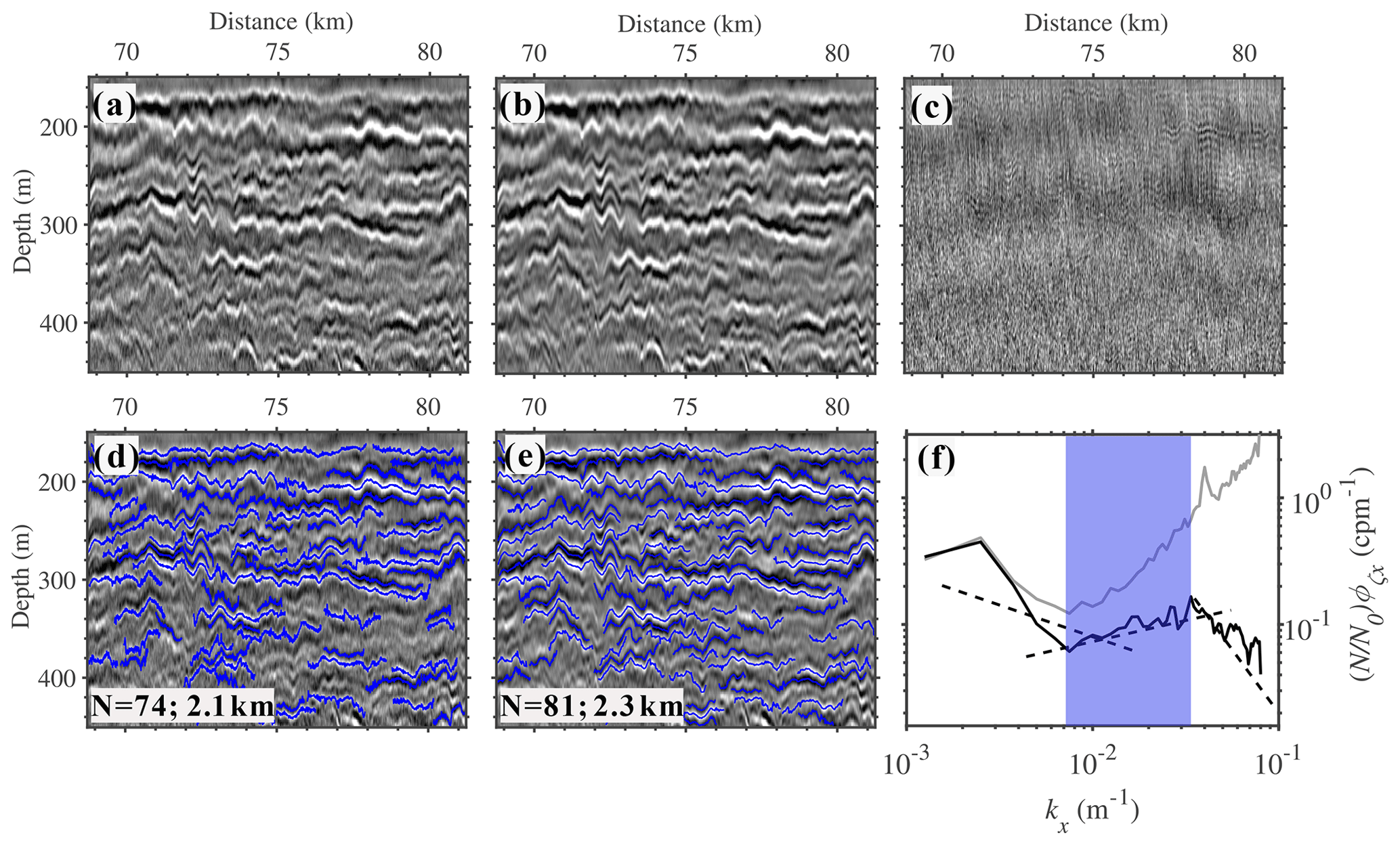
Figure 2 Example from seismic line 25 showing the effects of the bandpass filtering and notch filtering. (a) Original seismic data for the 68–81 km section. (b) After the bandpass filtering and notch filtering. (c) The difference between panels (a) and (b). (d, e) Tracked reflections (blue solid lines) from panels (a) and (b), respectively. (f) Slope spectra. The gray (black) line calculated from the tracked reflectors before (after) filtering of the seismic data.

2.2 Hydrographic data

Hydrographic data can be utilized to analyze local hydrographic characteristics and estimate the buoyancy frequency. In this study, due to the lack of synchronous hydrographic data, we used historical conductivity–temperature–depth (CTD) and expendable bathythermograph (XBT) data collected in September 2009, which are close to the acquisition time of the seismic data. Figure 3 shows the vertical variations of temperature, salinity, density, and buoyancy frequency with depth, derived from four CTDs. The buoyancy frequency N can be expressed as $\sqrt{-\frac{\mathit{\rho }}{g}\frac{\mathrm{d}\mathit{\rho }}{\mathrm{d}z}}$, where ρ is the seawater density, g is the gravitational acceleration, and z is the seawater depth. The alignment direction of the nine XBT stations roughly corresponds to the survey line direction, allowing for an approximate assessment of changes in the thermocline depth with varying seawater depth.

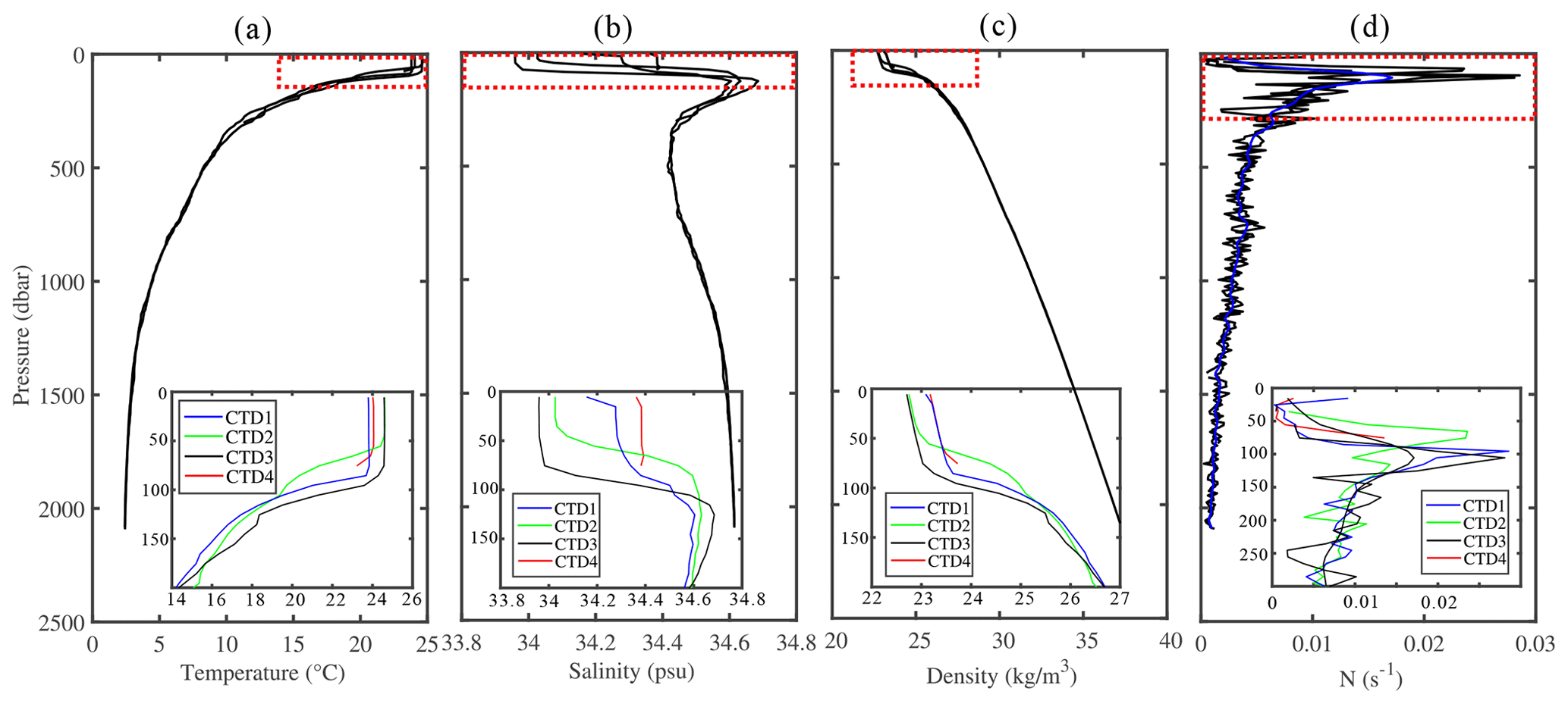
Figure 3 Data for temperature (a), salinity (b), density (c), and buoyancy frequency (d) from four CTD stations (see the station distribution in Fig. 1b). The insets in each graph (a–d) show data from a depth of 200–300 m within the red dashed-line boxes. The thick blue solid line in graph (d) represents the average buoyancy frequency of seawater.

2.3 Geostrophic shear estimation

To estimate the geostrophic velocity in the density field, it is necessary to assume that the Coriolis force and the horizontal pressure gradient force are balanced. The Rossby number $R_{\mathrm{0}}=U/fL$ should be much less than 1, where U is the characteristic velocity and L is the characteristic length. Under such geostrophic balance conditions, the density layers within the water column tend to tilt. In two-dimensional transects, the vertical shear S of the horizontal velocity perpendicular to the density field is determined using the standard thermal wind equation based on the slope of the isopycnal (McWilliams, 2006). Thus,

$$\begin{array}{}\text{(2)}& S={\displaystyle \frac{g}{{\mathit{\rho }}_{\mathrm{0}}f}}{\displaystyle \frac{\partial \mathit{\rho }}{\partial z}}\tan \mathit{\gamma },\end{array}$$

where g=9.8 m s⁻² is the gravitational acceleration, ρ₀ is the mean density of two layers, $\frac{\partial \mathit{\rho }}{\partial z}$ is the vertical gradient of density across the isopycnal, f is the Coriolis parameter, and γ is the slope of the isopycnal. Krahmann et al. (2009) demonstrated that the slope of the isopycnal measured using a yoyo CTD probe matches the slope of the reflections from the seismic data within 4 h. Given that the average speed of the vessel is 2.5 m s⁻¹ and within a certain length range (∼36 km), these reflections coincide with the isopycnal. Therefore, we can use seismic data to obtain the slope of the reflections as an approximation of the isopycnal slope γ.

In the study area, U≈0.1 m s⁻¹, $f\approx \mathrm{5}\times {\mathrm{10}}^{-\mathrm{5}}$ s⁻¹, and, for R₀=1, L=2 km. To ensure R₀≪1, we can grid the seismic transect with each window sized at 10 km×75 m (length × width), i.e., L=10 km, and an automatic picking algorithm is used to identify the seismic reflections within each window. The specific estimation method is referred to in previous works (Sheen et al., 2011; Tang et al., 2020).

2.4 Turbulent dissipation and diapycnal diffusivity estimates from seismic data

Klymak and Moum (2007) used horizontal wavenumber spectra from oceanic horizontal towed measurements to estimate the diapycnal diffusivity (K_ρ) in seawater. In the open ocean, the horizontal wavenumber spectrum (ϕ_ζ) can be clearly divided into two parts: the low wavenumber part is related to internal waves (${\mathit{\varphi }}_{\mathit{\zeta }}^{\text{IW}}$), with spectral characteristics consistent with the Garrett and Munk (1975) model (GM75) and proportional to the −2.5 power of the wavenumber, and the high wavenumber part is dominated by turbulence (${\mathit{\varphi }}_{\mathit{\zeta }}^{\mathrm{T}}$), exhibiting Kolmogorov-like behavior (proportional to the $-\mathrm{5}/\mathrm{3}$ power of the wavenumber).

Compared with the internal wave subrange, diapycnal diffusivity values computed from the turbulent subrange are probably more robust (Klymak and Moum, 2007a; Sheen et al., 2009). Therefore, we choose the turbulent subrange of the slope spectra to estimate diapycnal mixing in this study. The horizontal wavenumber spectra in the turbulent subrange can be represented by the simplified Batchelor (1959) model (Eq. 4), so the turbulence kinetic energy dissipation rate (ε) can be obtained from the horizontal wavenumber spectra. According to Eq. (5), the diffusivity K_ρ can be obtained (Osborn, 1980):

$$\begin{array}{}\text{(3)}& {\displaystyle }{\mathit{\varphi }}_{\mathit{\zeta }}^{\mathrm{T}}={\displaystyle \frac{\mathrm{4}\mathit{\pi }\mathrm{\Gamma }}{N^{\mathrm{2}}}}{C}_T{\mathit{\epsilon }}^{\mathrm{2}/\mathrm{3}}(\mathrm{2}\mathit{\pi }{k}_x{)}^{-\mathrm{5}/\mathrm{3}},\text{(4)}& {\displaystyle }{K}_{\mathit{\rho }}=\mathrm{\Gamma }\mathit{\epsilon }/N^{\mathrm{2}},\end{array}$$

where Γ≈0.2 is the mixing efficiency of seawater, C_T≈0.4 is considered a constant, and N is the average buoyancy frequency at the corresponding water depth.

Assuming that the isopycnals of seawater coincide with the seismic reflectors (Holbrook et al., 2013; Sheen et al., 2009; Krahmann et al., 2009), the horizontal wavenumber spectra obtained from the vertical displacement of reflectors can replace those obtained from horizontal towed measurements; thus, the turbulence dissipation rate and diapycnal diffusivity can also be calculated from seismic data. (e.g., Dickinson et al., 2017; Gong et al., 2021b; Tang et al., 2021; Yang et al., 2023). The steps are as follows. Firstly, an automatic picking algorithm is used to pick seismic reflectors in the seismic data, and the length of the reflectors should be no less than 1 km, totaling 410 reflectors (Fig. 4a). Then the vertical displacement of the picked reflectors is obtained by subtracting their linear fit curves, and the power spectral density of the displacement curve, i.e., the horizontal wavenumber spectrum (${\mathit{\varphi }}_{\mathit{\zeta }}^{\mathrm{T}}$), is calculated using a Fourier transform. The spectral calculation process uses a 128-point sampling point width and a nonoverlapping Hanning window. To better distinguish the internal wave subrange from the turbulence subrange, the displacement spectrum (${\mathit{\varphi }}_{\mathit{\zeta }}^{\mathrm{T}}$) is usually multiplied by (2πk_x)² to obtain the slope spectrum (${\mathit{\varphi }}_{{\mathit{\zeta }}_x}^{\mathrm{T}}$), so the slope of the turbulence subrange changes from $-\mathrm{5}/\mathrm{3}$ to $\mathrm{1}/\mathrm{3}$ and the slope of the internal wave subrange changes from $-\mathrm{5}/\mathrm{2}$ to $-\mathrm{1}/\mathrm{2}$ (Holbrook et al., 2013). After obtaining the slope spectra, we use the least-squares method to fit the spectra in the turbulent subrange (0.0075–0.0378 m⁻¹, blue-shaded area in Fig. 4c) and obtain fitted spectra to ensure the stability of the results. Finally, the fitted spectrum is substituted into Eqs. (3) and (4) to obtain the turbulent dissipation rate and diapycnal mixing. Additionally, to eliminate the influence of seawater stratification (N) on the internal wave field, we need to normalize the slope spectra according to the local average buoyancy frequency, i.e., multiply them by $N/N_{\mathrm{0}}$, where N is derived from Fig. 3d (N₀=3 cph).

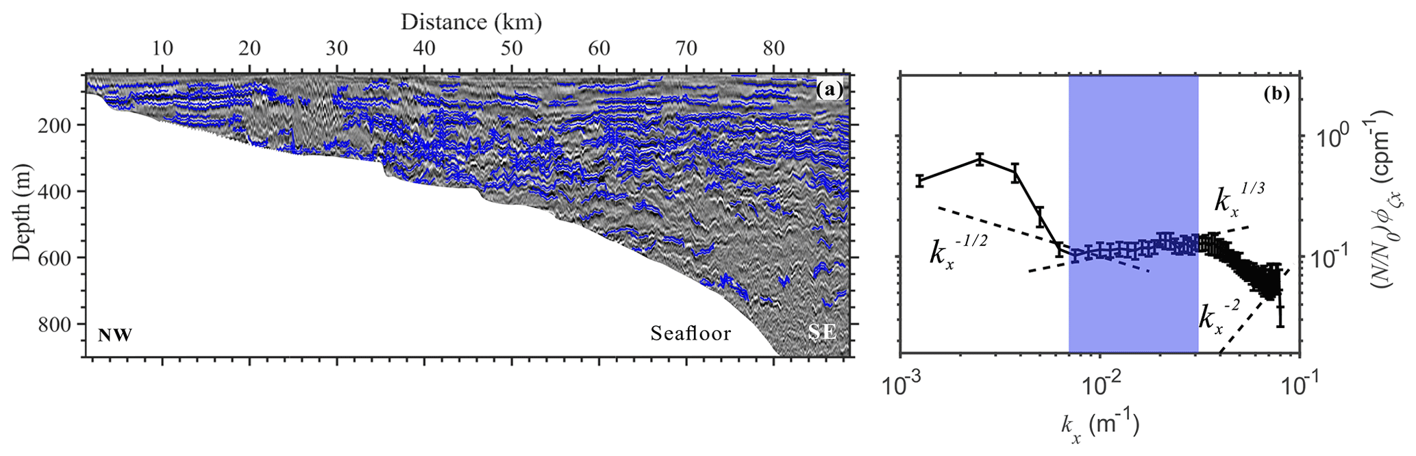
Figure 4 Picked reflections and the slope spectrum. (a) Picked reflectors from seismic line 25 (blue solid lines). (b) Slope spectrum calculated from the reflectors in Fig. 4a, with a 95 % confidence interval. The black dashed lines with $-\mathrm{1}/\mathrm{2}$ and $\mathrm{1}/\mathrm{3}$ slopes correspond to the theoretical slopes of GM75 for the internal wave subrange and the Batchelor model for the turbulence subrange, respectively. The black dashed line with a −2 slope is the noise subrange. The blue shaded area represents the turbulent subrange for fitting the spectrum.

To obtain the spatial distribution of the mixing parameters, we gridded the seismic transect of seismic line 25, with each window size being 5 km×75 m (length × width), the lateral step size being 2.5 km, and the vertical step size being 37.5 m. The average value within each window is taken as the dissipation rate and diffusivity for that window, following the previously mentioned method. Moreover, we interpolated and smoothed the data appropriately to ensure the spatial distribution's continuity.

3 Results

3.1 Seismic observations

Figure 5a shows the seismic image obtained through the aforementioned standard processing procedure. We observe that, in the shallow water region above 420 m, the seismic reflection signal is strong and the reflections are laterally continuous. In contrast, in deeper waters (>500 m), the reflection amplitude is relatively weaker, the reflections lose their continuity, and both their number and length are relatively reduced, especially in the deeper water between 70 and 89 km. Horizontally, the seismic reflections also exhibit some differences. Likely influenced by the seafloor topography, the reflections on the left side of the seismic image (1.25–55 km) show significant spatial morphological changes, with waveforms displaying high-frequency oscillations and breaking. Some reflections develop in an inclined manner. The reflections on the right side of the image (60–89 km) are mostly horizontally distributed, with the frequency and amplitude of the internal waves far less pronounced than those on the left.

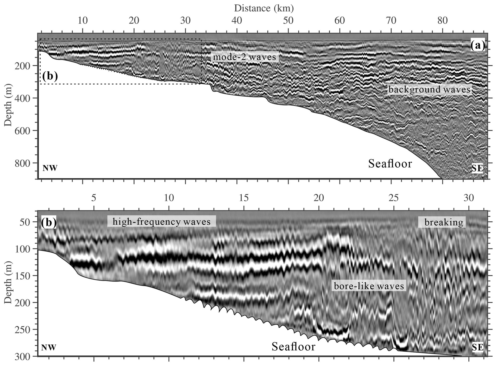
Figure 5 Seismic image of the internal waves. (a) Seismic image of line 25. Background waves and mode-2 waves are denoted. (b) The 1.25–33 km section of the image (a). High-frequency waves, bore-like waves, and breaking waves are denoted.

Figure 5b is an enlarged view of the 1.25–33 km section of the image. Within 20 km, the seismic image shows a series of high-frequency internal waves characterized by small-amplitude and high-frequency oscillations. The reflections gradually increase from left to right, with more evident seawater stratification. Adjacent to the high-frequency internal waves (20–26 km), we can see two bore-like waves with relatively larger amplitude and wave width. These convex-shaped reflective structures also remind us of high-mode internal waves, which are discussed in Sect. 4. After the first bore-like wave (21–24 km), the seismic reflections temporarily return to the original stratification in the ocean. However, following the appearance of the second wave, the trailing edge becomes unstable, with the right side of the waveform incomplete, and the reflections become intermittent and inclined (26.5–30 km). This indicates that internal wave breaking has occurred, which disrupts the original density stratification.

3.2 Satellite images

The actual data acquisition date for seismic line 25 was 31 July 2009. We collected recent MODIS images of the Dongsha waters, with Fig. 6a captured by the Aqua satellite on 29 July and Fig. 6b by the Terra satellite on 30 July. The alternating bright and dark stripes on these images represent the sea surface manifestations of ISW packets. Both wave packets exhibit long wave crests, and the convex curvature of these crests indicates their northwestward propagation on the shoaling continental shelf, sequentially passing through seismic line 25 (indicated by the red solid line). Each pair of adjacent bright and dark stripes corresponds to the leading and trailing edges of the wave, with the distance between them representing the wave width. The satellite images show that the wave width of both packets gradually decreases from the leading wave until it becomes indistinguishable. Notably, the number of identifiable solitons is significantly greater in the first packet compared to the second one. This suggests that ISW packets near seismic line 25 are well-developed and propagate northwestward along the line direction on the continental shelf. The HIWs observed in the seismic image may result from the fission of these wave packets. However, due to the limited resolution (250 m), these features cannot be fully identified from the remote sensing images.

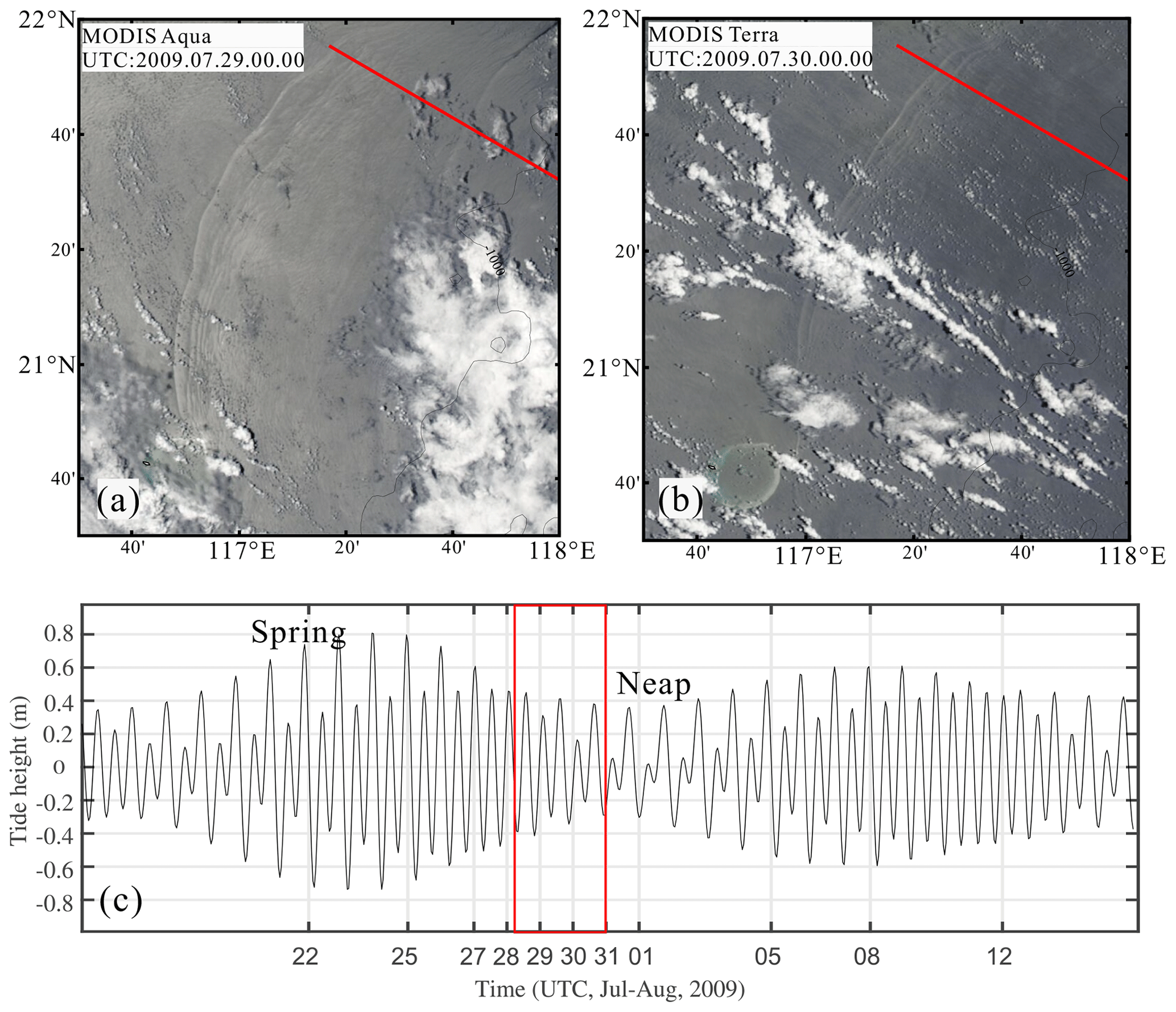
Figure 6 Satellite images and tidal model. (a) MODIS image collected by the Aqua satellite in the northern South China Sea on 29 July 2009. (b) MODIS image collected by the Terra satellite in the northern South China Sea on 30 July 2009. (c) Tidal height time series near the Luzon Strait (20.6° N, 121.9° E) from 14 July to 14 August 2009. The red box indicates the time period used to infer the generation of ISWs.

Figure 6c shows the total tidal height time series near the Luzon Strait (20.6° N, 121.9° E) from 14 July to 14 August 2009. These data are derived from the global ocean tide model TPXO9 developed by Oregon State University (Egbert and Erofeeva, 2002), which provides 15 tidal constituents (M2, S2, N2, K2, K1, O1, P1, Q1, Mm, Mf, M4, Mn4, Ms4, 2n2, and S1). The propagation speed of internal waves is influenced by various factors, including background currents, water stratification, and changes in bottom topography, resulting in different speeds at different depths. Generally, internal waves propagate fastest in deep-sea areas, exceeding 3 m s⁻¹. As they propagate towards the continental shelf, their speed decreases to 1–2 m s⁻¹ (Alford et al., 2010; Cai et al., 2014). The distance from this point to the HIWs observed in the seismic image is approximately 500 km. Assuming an average speed of 2 m s⁻¹, it would take about 69 h to cover this distance. Therefore, we infer that these ISWs passing seismic line 25 may have originated during the neap tide period (indicated by the red box in Fig. 6c).

3.3 High-frequency internal waves

In fact, the thermocline may be shoaling, with the bottom shoaling on the continental slope or shelf. The density difference between the upper and lower layers of seawater also changes with the shoaling topography. Therefore, considering these environmental factors is crucial for explaining the evolution of ISWs. In September 2009, nine XBT data were collected, with their alignment direction roughly corresponding to the direction of seismic line 25 (Figs. 1a and 7). This allows for a rough estimation of the thermocline depth variation with changing seawater depth. We determine the thermocline depth by taking the middle depth between two inflection points in the temperature profile, where temperature changes significantly. Figure 8 shows the variations of thermocline depth and the temperature difference with water depth. We can observe that, except for XBT7, the thermocline shoals with the shoaling topography, with the depth decreasing from 127 to 57 m and the temperature difference between the upper and lower layers decreasing from 8.2 to 1.8 °C. From the perspective of wave dynamics, these changes can influence these waves' propagation characteristics in certain cases. Along the track, as the water depth decreases from 1800 to 20 m, Zheng et al. (2001) found that the thermocline shoals from 36 m in deep water to 13 m in shallow water. Simultaneously, the density difference between the upper and lower layers of seawater is reduced to half of its original value, which facilitates the shoaling of ISWs. The phase speed decreases from 0.85 m s⁻¹ in deep water to 0.27 m s⁻¹ in shallow water. Therefore, if we are interested in the shoaling of internal waves in the South China Sea, we cannot neglect the changes in the ocean's dynamic environment.

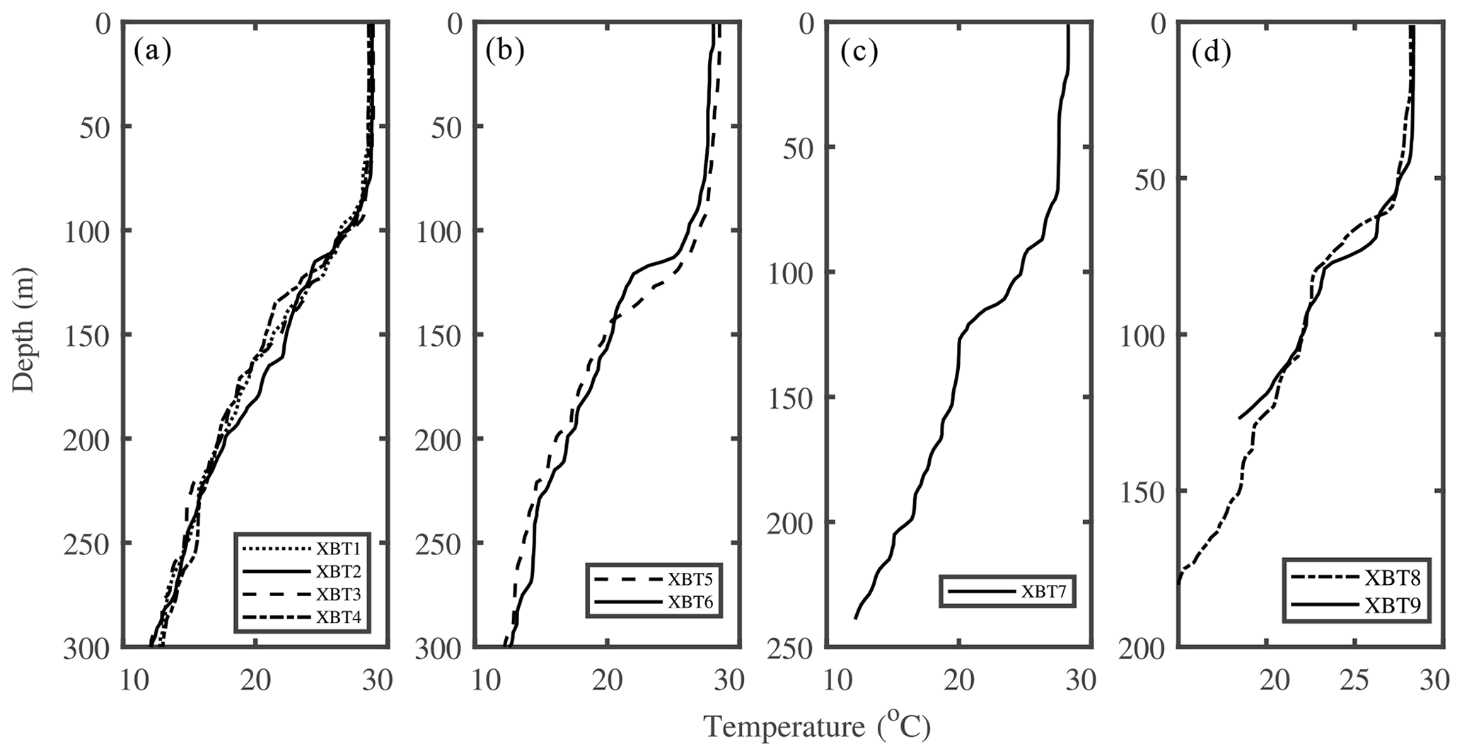
Figure 7 Temperature profiles from XBT. The distribution of XBT stations is listed in Fig. 1b.

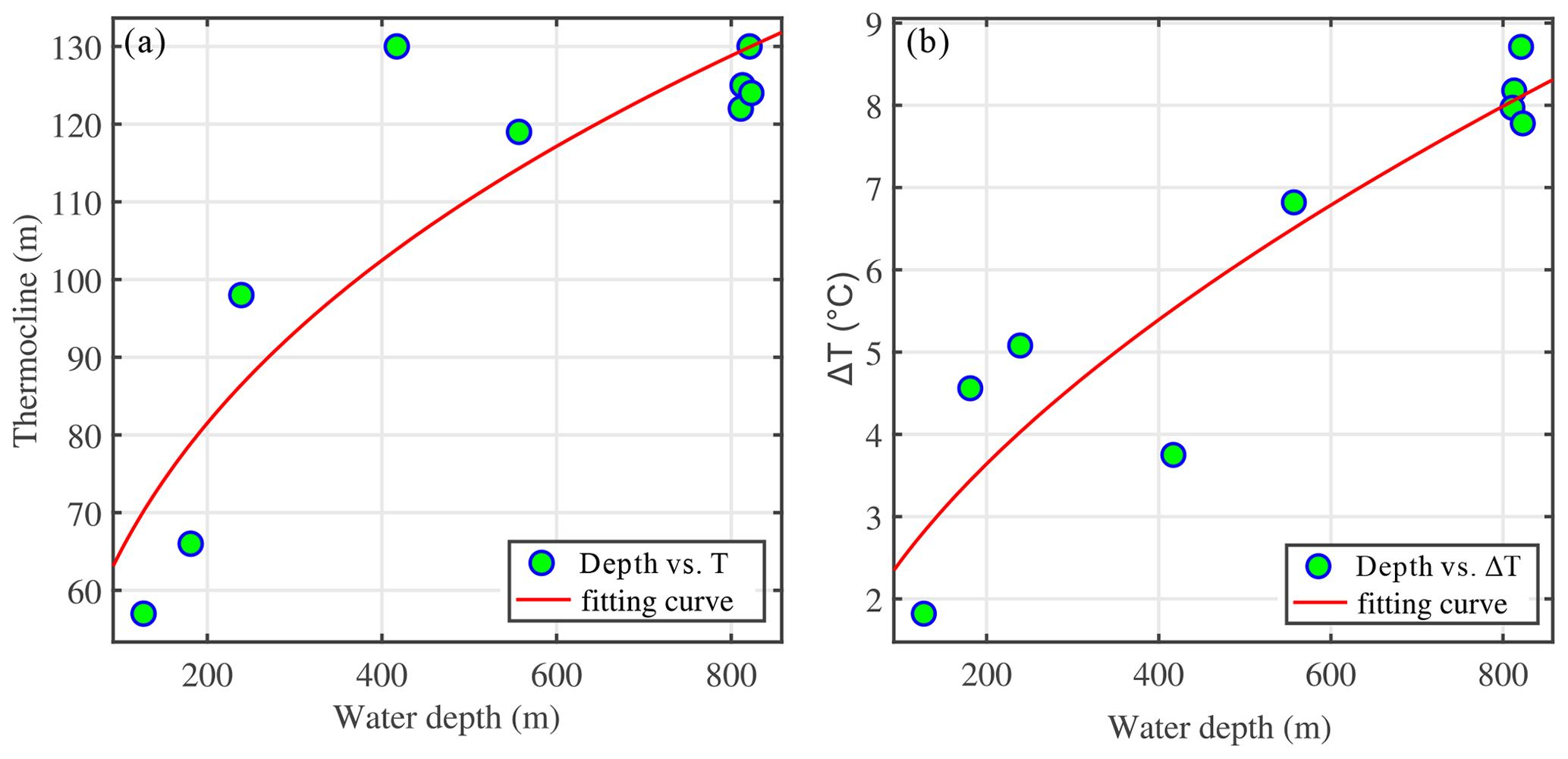
Figure 8 Variations of (a) thermocline depth and (b) temperature difference between the upper layer and lower layer with the shoaling water depth.

Geng et al. (2019) utilized the same multichannel seismic data to observe large-amplitude ISWs and analyze the relationship between the vertical structure of the waves and water depth. Gong et al. (2021a) conducted a detailed statistical analysis of the dynamic characteristics and waveform information of these waves from this cruise, including amplitude and wavelength (Tables 1 and 2 in Gong et al., 2021a). Unlike our observations, these waves are large-amplitude solitons that maintain the original shapes during propagation in deeper water (>350 m) and have not yet strongly interacted with the seabed, while we observed a series of small-amplitude, high-frequency internal waves on one of the seismic lines, which primarily developed near the topography. Here, we consider these symmetric, large-amplitude ISWs to be initial waves. Research indicates that internal wave breaking is directly related to both topography and waveform, which are commonly characterized by the internal Iribarren number (${\mathit{\xi }}_{\text{in}}=S/\sqrt{a/L_{\mathrm{w}}}$), where S is the seabed slope, a is the initial wave amplitude, and L_w is the initial wave's half-wavelength (Aghsaee et al., 2010). The seabed slope corresponding to seismic line 25 is known to be S=0.018 (Fig. 1b). Calculations show that the range of wave steepness $a/L_{\mathrm{w}}$ is 0.01–0.36 and that the range of ξ_in is 0.03–0.17. Therefore, ISWs may undergo fission under conditions of gentle slopes (S≤0.05) and low internal Iribarren numbers (Orr and Mignerey, 2003; Sinnett et al., 2022; Zheng et al., 2001). Additionally, $a/L_{\mathrm{w}}$ is generally proportional to the Froude number used to describe the degree of nonlinearity of internal waves. A ratio greater than 1 would result in seawater overturning (Masunaga et al., 2019), while here the value is less than 1. Therefore, the seabed slope is one of the key factors determining the shoaling and breaking of internal waves, which is consistent with the findings of other research (e.g., Boegman et al., 2005; Terletska et al., 2020; Vlasenko and Hutter, 2002).

The above observations can be summarized as follows. The thermocline depth is shoaling, and the temperature difference between the upper and lower layers also varies with bottom shoaling. The seabed slope is gentle enough to contribute to the fission. Bai et al. (2013, 2019) discovered that ISWs also undergo fission in the South China Sea shelf region, generating HIWs, which provides a new pathway for the energy dissipation of these waves. Therefore, the HIWs seen in Fig. 5b might also be the result of the fission. The high-frequency internal waves (packets) produced during the shoaling are mainly distributed within a depth range of 79–184 m, with an average amplitude of 7–9 m and a maximum amplitude of about 13 m. The half-height width ranges from 154 to 240 m, as detailed in Table 1. It is similar to the sizes of high-frequency internal waves observed by Bai et al. (2019). Near the thermocline, the reflections exhibit high-frequency oscillations and good horizontal continuity. Closer to the seabed, due to strong interactions between internal waves and topography, the reflections become distorted and gradually lose their horizontal continuity (horizontal distance 18–20 km, water depth 200–250 m).

Table 1 Waveform statistics of high-frequency ISWs.

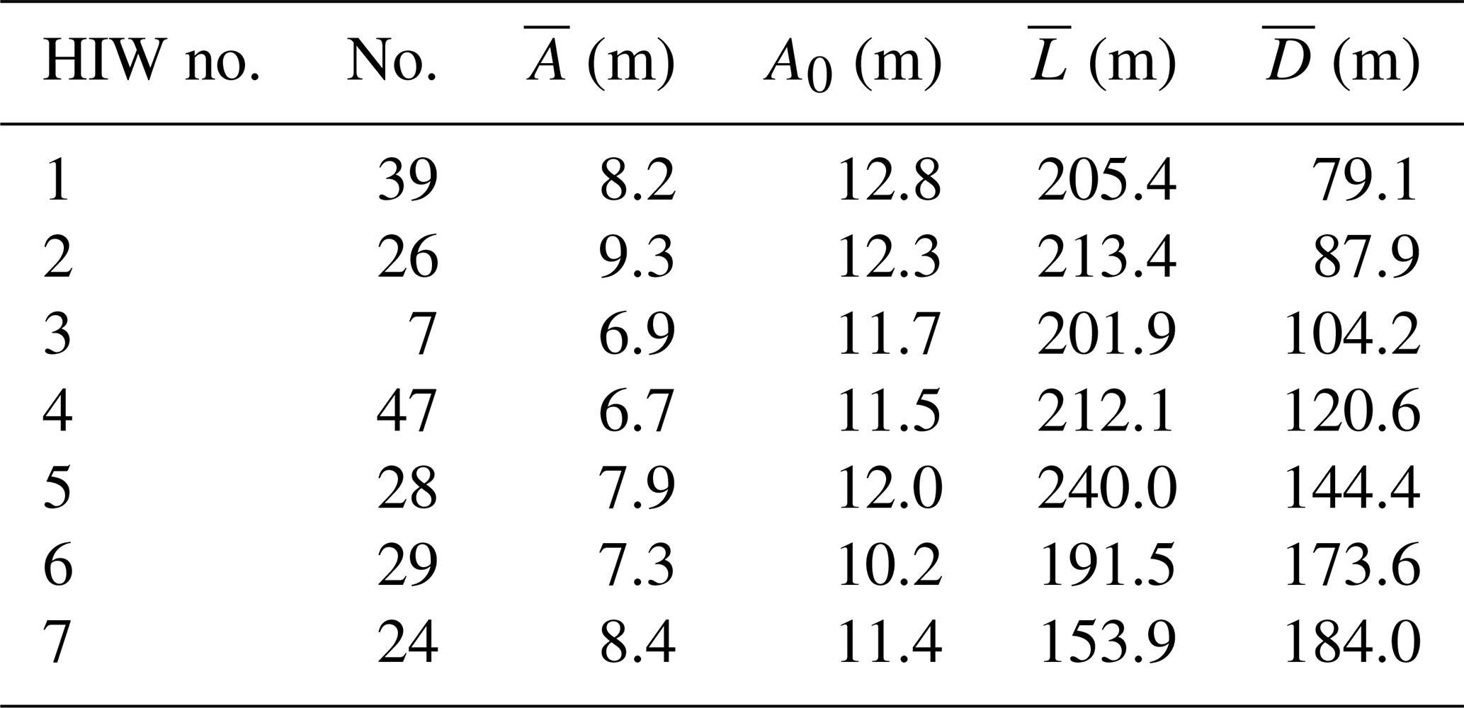
HIW no.: the number of high-frequency internal waves (packets). No.: the number of elevation waves in the packet. $\stackrel{\mathrm{‾}}{A}$: average amplitude. A₀: maximum amplitude in the packet. $\stackrel{\mathrm{‾}}{L}$: average half-height width. $\stackrel{\mathrm{‾}}{D}$: average depth of the packet location.

3.4 Geostrophic shear and shear instability

Based on geostrophic balance theory, we can estimate the vertical shear of horizontal velocity by tracking seismic reflectors. Vertical shear (in color) is superimposed on the seismic images (in gray) to better analyze the spatial distribution of shear. In Fig. 9a, the shear on the left sides of the seismic transects is significantly stronger than that on the right sides, and its strength often correlates positively with the inclination of seismic reflectors. In the high-frequency internal wave region (<20 km), the reflectors are horizontally distributed but exhibit high-frequency oscillations, resulting in an average shear of $\mathrm{5}\times {\mathrm{10}}^{-\mathrm{3}}$ s⁻¹. In regions with bore-like waves and internal wave breaking (20–30 km), the reflectors show large inclinations or even breaks, resulting in the highest shear across the transect of up to 0.03 s⁻¹. The reflectors are slightly inclined at 30–45 km due to the seabed topography, which also causes shear. The shear caused by the background waves gradually weakens from left to right (>70 km).

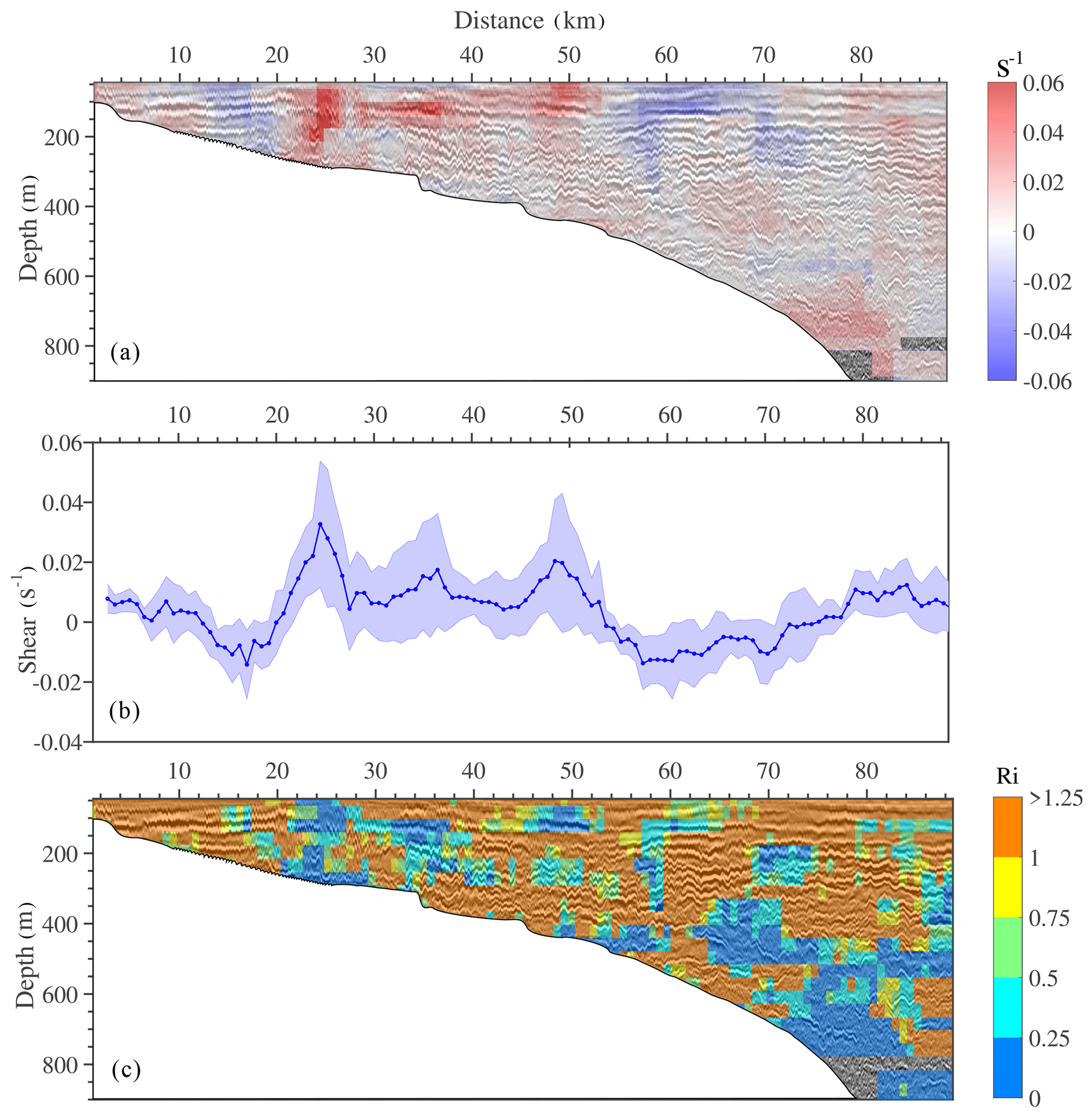
Figure 9 Geostrophic shear and Richardson number (Ri) estimated from seismic data. (a) Geostrophic shears (in color) are superimposed on the seismic images (in gray). Panel (b) represents the mean vertical shear (blue line) and the standard deviation (blue shading) for the depth of 50–200 m of the seismic transect. (c) Ri values are superimposed on the seismic images (in gray).

Shear instability can be quantified using the Richardson number $\mathit{Ri}=N^{\mathrm{2}}/S^{\mathrm{2}}$, where N is the buoyancy frequency and S is the geostrophic shear. Generally, an area is considered unstable when Ri<0.25 (Lamb et al., 2014). Here, we use the average buoyancy frequency obtained from historical CTD data as N and the shear estimated from seismic data as S. As shown in Fig. 9b, regions with Ri<0.25 account for about 8 % of the seismic image. In the 20–30 km range at depths of 150–250 m, weak stratification and strong shear cause the Richardson number (Ri) to be less than 0.25, indicating shear instability in the ocean. At depths of 500–800 m, Ri also drops below 0.25, likely due to sufficiently weak stratification or vertical oscillations of the reflectors. Additionally, the low signal-to-noise ratio in the deep water may cause some errors.

Kelvin–Helmholtz (KH) billows typically have an alternating braid–core structure resembling “cat's eyes” and often exhibit small-scale secondary instabilities in the braids (Thorpe, 1987). It is rare to see a complete cat's eye structure in the ocean; more often, this manifests as braid structures (Acabado et al., 2021; Chen et al., 2022; Chang et al., 2016; Geyer et al., 2010; Tu et al., 2022). In Fig. 10, we can clearly observe KH billows caused by instability in the seismic transect. These billows are distributed in the range of 26.5–30 km and are mostly inclined inverted “S” shapes, i.e., braid structures (blue solid line in Fig. 10b). Table 2 lists the details of some clearer billows: the amplitude is about 26–45 m, and the apparent wavelength is about 212–322 m. When less than 28 km, the reflectors are shorter and incomplete, which may be caused by high shear. When greater than 28 km, the braid structure is more evident. We can also extract the waveform information of KH billows from the seismic transect to estimate the aspect ratio and minimum Richardson number Ri_o (0.25–0.39 $h_{\text{es}}/\mathit{\lambda }$, where $h_{\text{es}}/\mathit{\lambda }$ is the ratio of wave height to wavelength), thereby roughly assessing the instability. Through calculation, the average aspect ratio is 0.13, and Ri_o averages 0.2, indicating conditions favorable for the occurrence of instability, which is consistent with the result of Fig. 9. Tu et al. (2022) estimated the turbulence dissipation rate ε ($C^{-\mathrm{2}}{h}_{\text{es}}^{\mathrm{2}}{N}^{\mathrm{3}}$, where C≈12.5) caused by KH billows using waveforms extracted from acoustic data. Here, we can apply this parameterization scheme to estimate the turbulence dissipation rate in the transect. The average dissipation rate is $\mathit{\epsilon }={\mathrm{10}}^{-\mathrm{6.7}\pm \mathrm{0.1}}$ m² s⁻³, indicating that shear instability plays an important role in the energy dissipation of ISWs.

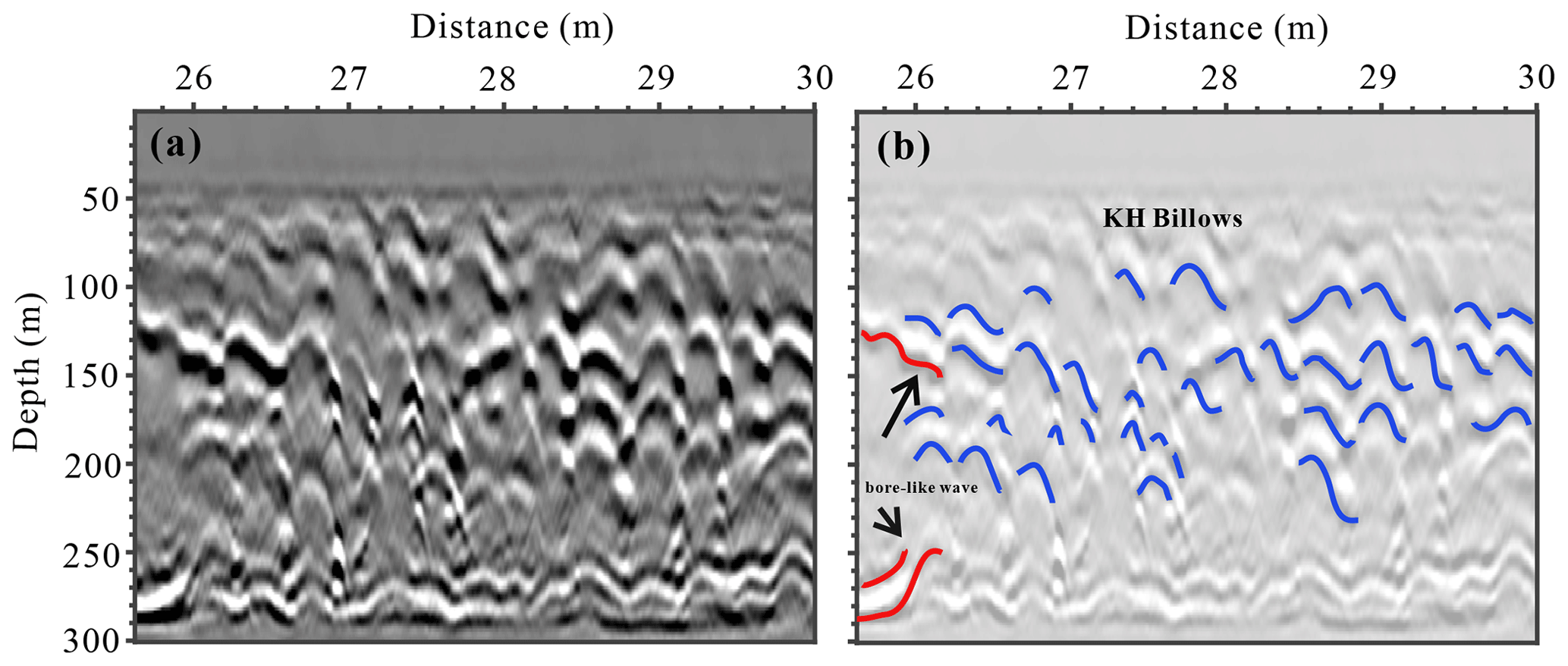
Figure 10 Structure of KH billows. (a) Enlarged view of the transect containing KH billows. (b) Interpretative diagram of the reflectors in the seismic image, where blue solid lines represent KH billows and red solid lines represent the rear wing of bore-like waves, whose waveform is not very complete due to instability.

Table 2 Statistics of KH billow waveforms.

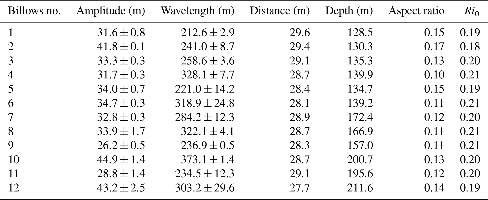
Billows no.: the number of KH billows. Amplitude: the amplitude (wave height) of the billows. Wavelength: the wavelength of the billows. Distance: the horizontal distance where the billows are located. Depth: the depth of the seawater where the billows are located.

3.5 Diapycnal diffusivity maps

We used the method mentioned in Sect. 2.4 to interpolate and smoothen the average dissipation rate (diapycnal mixing) calculated for each window with the values from the surrounding windows. We obtained Fig. 11 by overlaying the results on the seismic image. This makes it easier to not only grasp the spatial distribution of the calculation but also to understand the correspondence between the results and the seismic image. Figure 12 is a histogram of the dissipation rate (diapycnal mixing) over different horizontal ranges. An analysis of the fitting errors is detailed in Appendix A.

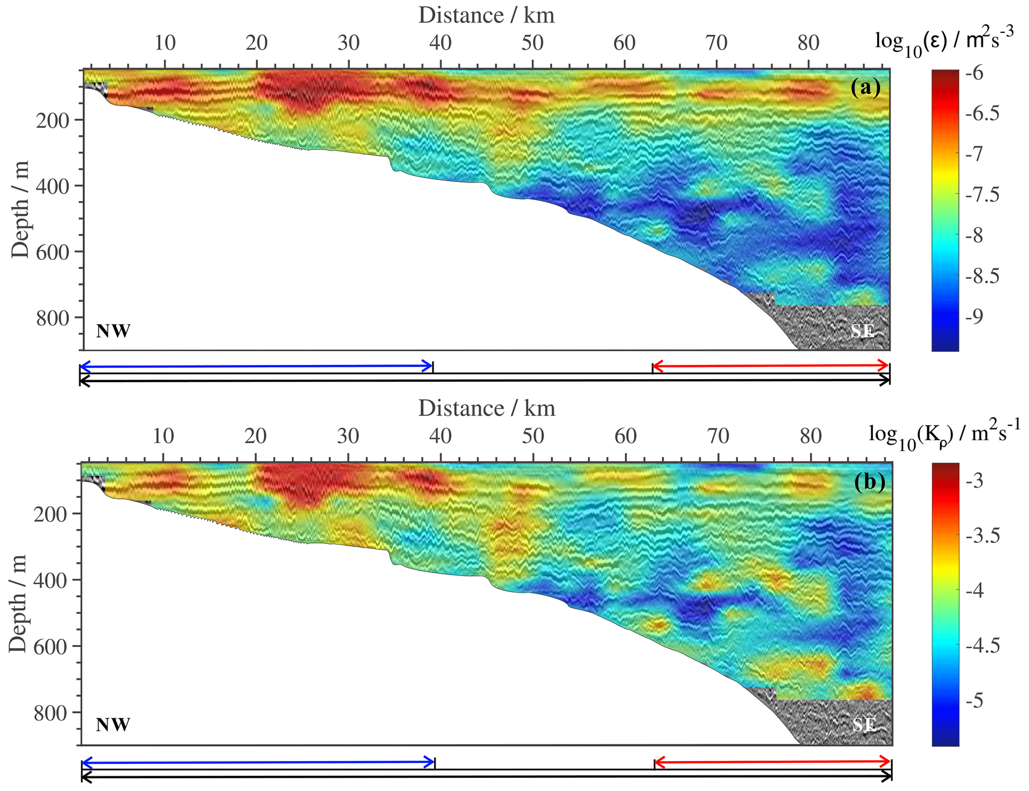
Figure 11 Distribution map of mixing parameters. (a) Spatial distribution of the turbulence dissipation rate. (b) Spatial distribution of diapycnal mixing, where the blue arrow represents the horizontal range of 1.25–38.75 km, the red arrow represents the horizontal range of 62.5–88.75 km, and the black arrow represents the horizontal range of 1.25–88.75 km.

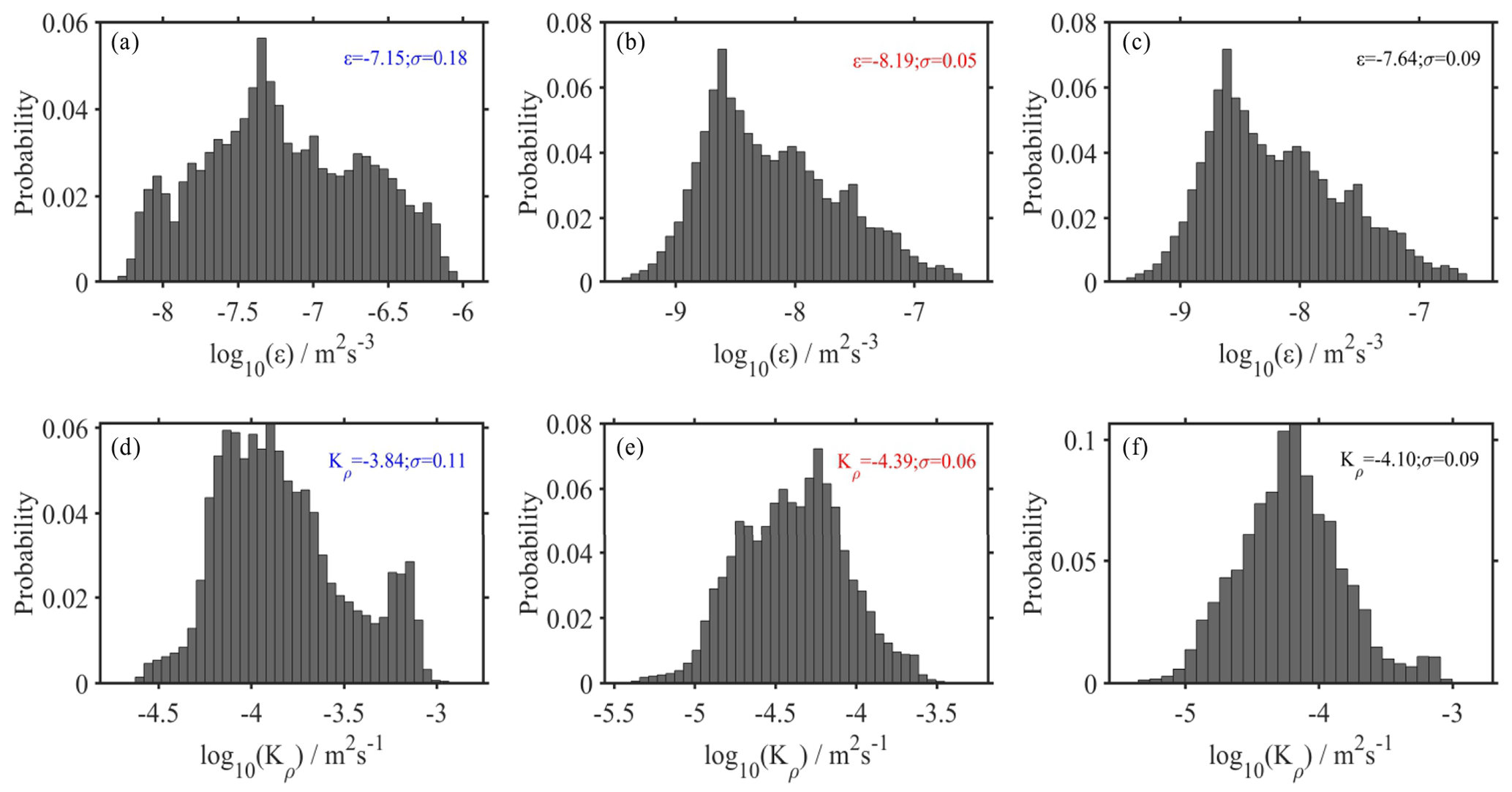
Figure 12 Panels (a) and (d) are distribution histograms of the dissipation rate and diapycnal mixing, respectively, for the range indicated by the blue arrow (1.25–38.75 km) in Fig. 11. Panels (b) and (e) are distribution histograms of the dissipation rate and diapycnal mixing, respectively, for the range indicated by the red arrow (62.5–88.75 km) in Fig. 11. Panels (c) and (f) are distribution histograms of the dissipation rate and diapycnal mixing, respectively, for the range indicated by the black arrow (1.25–88.75 km) in Fig. 11.

According to Figs. 11 and 12, we find that the mean diapycnal mixing is ${\mathrm{10}}^{-\mathrm{4.10}\pm \mathrm{0.09}}$ m² s⁻¹ (−4.10 is the average and 0.09 is the standard deviation), which is 1 order of magnitude greater than the average in the open ocean (10⁻⁵ m² s⁻¹). In the upper layer of seawater (above 200 m), especially near the thermocline, the dissipation rate (diapycnal mixing) is high, while below 200 m the dissipation rate (diapycnal mixing) decreases with increasing depth. However, the dissipation rate (diapycnal mixing) is also high near the seabed. The calculated diapycnal mixing for the 1.25–38.75 km range is ${\mathrm{10}}^{-\mathrm{3.84}\pm \mathrm{0.11}}$ m² s⁻¹, which is 3.5 times greater than the calculation for the 62.5–88.75 km range (10^−4.39 m² s⁻¹). As we discussed earlier, a series of shoaling events occurred within the 1.25–38.75 km range: the HIWs can enhance the diapycnal mixing, averaging 10⁻⁴ m² s⁻¹. In the range of 20–30 km, a marked increase in K_ρ suggests that enhanced mixing is associated with the breaking of IWs caused by the strong shear. The red patches have a slightly deeper color than the other area, indicating that this is a high mixing area in the transect, up to 10⁻³ m² s⁻¹. When away from the topography (62.5–88.75 km), the mixing weakens.

The results suggest that HIWs generated from the shoaling ISWs can also enhance turbulent dissipation and mixing. The elevated velocity shear during the shoaling may cause the occurrence of shear instability. The results of numerical simulations by Bai et al. (2019) support this point: they indicate that the shear within the thermocline intensifies significantly when ISWs fission into HIWs, and the shear instability resulting from strong shear may cause the enhanced diapycnal mixing. Therefore, the fission of ISWs into HIWs is one of the key processes in the energy dissipation of these waves.

4 Discussion

4.1 Internal structure of the bore-like nonlinear waves

As shown in Fig. 13, we observe nonlinear waves (NIWs) with complex structures and shapes like bores. The upper boundary of these two “convex”-structured reflectors is convex upwards, while the lower boundary is concave downwards. Compared to the strong reflectors at the boundaries, the core is transparent or weakly reflective, with a central depth of around 180 m and a thickness of about 150 m, indicating well-mixed water.

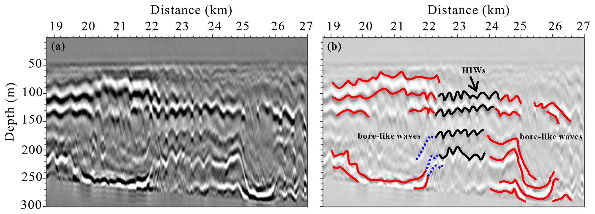
Figure 13 Bore-like NIWs. (a) Enlarged view of the 19–27 km transects in Fig. 5. (b) Interpretative diagram of the reflectors in the seismic image, where red solid lines represent the boundaries of NIWs, black solid lines represent HIWs, and blue dashed lines indicate hydraulic jumps.

At around 20 km, the reflectors no longer remain horizontal. The reflectors of the upper boundary gradually become convex upwards, with a displacement of about 70 m, and the lower boundary becomes concave downwards, with a displacement of about 50 m. In contrast, the upper and lower boundaries at the wave's rear (around 22 km) have opposite displacements, forming the bore-like NIW. At 22–24 km, the seawater at the rear gradually returns to its original stratification due to the hydraulic jump, and HIWs reappear. However, another similarly shaped NIW appears about 2 km behind. The upper boundary of this wave is more diffuse, and the lower-boundary layer is concave down to near a depth of 290 m, with a displacement of about 100 m. Unlike the former, the reflectors at the rear (∼26 km) do not return to the original stratification but become disordered and breaking, representing the enhanced turbulence state in the ocean.

4.2 Mode-2 ISWs or shoaling bores?

Utilizing field observations and numerical simulations, Scotti et al. (2008) found that strong nonlinear HIWs interacting strongly with shoaling topography in Massachusetts Bay can result in “seabed collision events”. Specifically, they found that, under conditions of gentle slope and moderate amplitude, these waves would undergo high-energy collision events. The waveforms generated in these collisions are remarkably similar to those observed in Fig. 13 and are often accompanied by the occurrence of hydraulic jumps. Thus, we speculate that such complex wave packets may represent a form of internal wave deformation during seabed collision events.

There are two speculations about what they are exactly. Firstly, shoaling internal waves usually form bores with bottom-enclosed structures carrying cold water masses that continue to propagate shoreward after breaking (Jones et al., 2020). The strength and structure of bores are influenced by the background stratification and the depth of the thermocline (if $(A+z_{\text{th}})/h>\mathrm{1}/\mathrm{2}$, shoaling internal waves will form bores, where A is the amplitude of an ISW, z_th is the thermocline depth, and h is the water depth) (Scotti et al., 2008; Sinnett et al., 2022; Walter et al., 2014). Bores typically begin to dominate the structure of internal waves near depths less than 50 m, becoming a primary feature of the wave during the shoaling process (McSweeney et al., 2020). However, the two complex wave packets in this paper are located at a depth of 300 m. Therefore, we believe that, although the structure of the two wave packets is somewhat similar to that of bores, their distribution depth range does not align with the typical distribution depth of common bores, which are often in shallower regions in the run-up phase. Another explanation is that they are high-mode NIWs. It is worth noting that the apparent wave width range of these two NIWs is 1.5–2 km, with an amplitude range of 50–100 m, which is clearly larger than the size of the mode-2 internal solitary waves found by Yang et al. (2010) in the South China Sea shelf and slope areas (with amplitudes of 20–30 m and an average timescale of 6.9–8 min). According to simulations by Brandt and Shipley (2014), we think that they might belong to exceptional large-amplitude internal solitary waves.

4.3 Dissipation mechanism of ISWs in the South China Sea

Previous extensive studies have shown that shoaling ISWs enhance the mixing of seawater (Gong et al., 2021b; Moum et al., 2007). Lamb (2014) summarized four scenarios in which shoaling ISWs enhance mixing: (1) Vertical shear caused by waves leads to shear instability, usually occurring in areas where Ri<0.25. (2) Convective instability occurs when the velocity of the water mass exceeds the phase velocity, often accompanied by enclosed vortex cores, within which the water is unstable and in a turbulent state. (3) Instability near the seabed boundary layer causes sediment resuspension and transport. (4) Direct breaking occurs when encountering steep terrain during the shoaling process.

In this study, our observational results demonstrate a new energy cascade route from shoaling ISWs to turbulence, deepening our understanding of the energy dissipation process of ISWs and their roles in enhanced mixing in the northern South China Sea (SCS). We find that the fission of ISWs into HIWs on the continental slope or shelf is also an important pathway for the tidal energy cascade. The HIWs generated during the shoaling can also enhance turbulent dissipation and mixing, on average causing diapycnal mixing on the order of 10⁻⁴ m s⁻¹. The results are consistent with previous research by Bai et al. (2013, 2019).

5 Conclusions

In this study, we employed seismic methods to investigate the shoaling evolution and energy dissipation mechanisms of ISWs. We observed HIWs along seismic line 25, which were primarily distributed in the depth range of 79–184 m. Their amplitudes are O (10 m), with half-widths ranging from 154 to 240 m. The MODIS image revealed that ISWs from the Luzon Strait typically appeared as wave packets near seismic line 25 during the data collection period, with tidal models indicating that these waves originated during the neap tide. Fission generally applies to gentle slopes with low ξ_in. Calculations show that the seabed slope corresponding to seismic line 25 is S=0.018 (≤0.05), with ξ_in ranging from 0.03 to 0.17. Therefore, we infer that HIWs are products of the fission of shoaling ISWs. Within the 20–30 km range of the transect, there are two complex bore-like nonlinear waves resulting from strong interactions between nonlinear waves and the topography. At the trailing edge of the second nonlinear wave, the reflectors appeared disordered and even fragmented, with KH billows forming. The amplitudes of these billows ranged from 26 to 45 m, with wavelengths between 212 and 322 m. By combining seismic and hydrological data, we estimated the geostrophic shear and Richardson number. We found that, in the 20–30 km range, vertical shear could reach up to 0.3 s⁻¹, with an Ri value of less than 0.25, indicating the occurrence of shear instability. Therefore, when shoaling ISWs undergo fission into HIWs, the enhanced shear within the seawater contributes to shear instability.

We used seismic data to estimate the mixing parameters of seawater and found that diapycnal mixing for the 1.25–38.75 km range is ${\mathrm{10}}^{-\mathrm{3.84}\pm \mathrm{0.11}}$ m² s⁻¹, which is 3.5 times greater than the calculation for the 62.5–88.75 km range (10^−4.39 m² s⁻¹). A series of shoaling events occurred within the 1.25–38.75 km range: the HIWs can enhance the diapycnal mixing, averaging 10⁻⁴ m² s⁻¹. In the range of 20–30 km, a marked increase in K_ρ suggests enhanced mixing associated with breaking of IWs caused by the strong shear of up to 10⁻³ m² s⁻¹. When away from the topography (62.5–88.75 km), the mixing weakens. Our observational results show a new energy cascade route from shoaling ISWs to turbulence, i.e., the fission of ISWs into HIWs, which improves our knowledge of ISW energy dissipation and its role in improved mixing in the northern SCS.

Appendix A: Error analysis

Generally speaking, there is a certain error between the fitted spectrum obtained by the least-squares method and the actual spectrum, which we represent here using the standard deviation σ. Therefore, we can obtain the upper and lower limits of the turbulence dissipation rate (diapycnal mixing) (Fig. A1).

Additionally, the selection of different parameter values in Eqs. (3) and (4) will result in errors in the outcome. We typically take the 95 % confidence interval of the average buoyancy frequency (Fig. 3d), so the error in the diapycnal mixing in the log domain is about 0.02 m² s⁻¹. The range of the mixing efficiency Γ is 0.1–0.4 (Mashayek et al., 2017), and here we take 0.2, causing an error in the diapycnal mixing in the log domain of about 0.15 m² s⁻¹. The range of C_T values is 0.3–0.5 (Sreenivasan, 1996), and here we take 0.4, resulting in an error in the diapycnal mixing of about 0.14–0.17 m² s⁻¹ in the log domain.

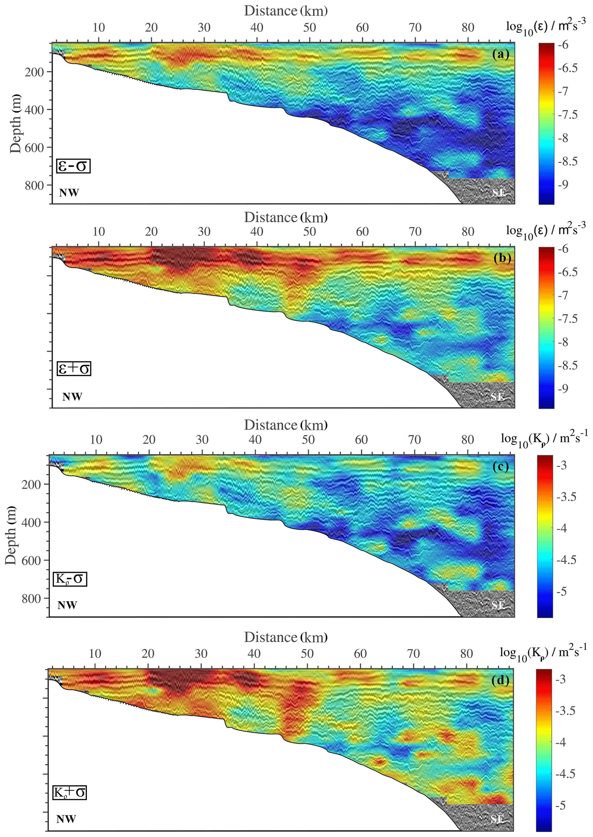
Figure A1 (a) ε−σ. (b) ε+σ. (c) K_ρ−σ. (d) K_ρ+σ. ε is the turbulence dissipation rate, K_ρ is the diapycnal mixing, and σ is the standard deviation for the fitting spectrum.