Multifractal structure and Gutenberg–Richter parameter associated with volcanic emissions of high energy in Colima, Mexico (years 2013–2015)

The evolution of multifractal structures in various physical processes, such as climatology, seismology, or volcanology, serves as a crucial tool for detecting changes in corresponding phenomena. In this study, we explore the evolution of the multifractal structure of volcanic emissions with varying energy levels (observed at Colima, Mexico, during the years 2013–2015) to identify clear indicators of imminent high-energy emissions nearing 8.0×10⁸ J. These indicators manifest through the evolution of six multifractal parameters: the central Hölder exponent (α₀); the maximum and minimum Hölder exponents (α_max, α_min); the multifractal amplitude ($W={\mathit{\alpha }}_{\text{max}}-{\mathit{\alpha }}_{\text{min}}$); the multifractal asymmetry ($\mathit{\gamma }=[{\mathit{\alpha }}_{\text{max}}-{\mathit{\alpha }}_{\mathrm{0}}]/[{\mathit{\alpha }}_{\mathrm{0}}-{\mathit{\alpha }}_{\text{min}}]$); and the complexity index (CI), calculated as the sum of the normalized values of α₀, W, and γ. Additionally, the results obtained from adapting the Gutenberg–Richter seismic law to volcanic energy emissions, along with the corresponding skewness and standard deviation of the volcanic emission data, further support the findings obtained through multifractal analysis. These results, derived from multifractal structure analysis, adaptation of the Gutenberg–Richter law to volcanic emissions, and basic statistical parameters, hold significant relevance in anticipating potential volcanic episodes of high energy. Such anticipation can be further quantified using an appropriate forecasting algorithm.

1 Introduction

The application of fractal and multifractal theory to Earth sciences (Goltz, 1997; Turcotte, 1997; Karsten et al., 2005, among others) represents an intriguing avenue for analyzing complex geophysical and atmospheric phenomena, serving as a significant step in the forecasting process. Examples include studying rainfall patterns (Koscielny-Bunde et al., 2006; Lana et al., 2017, 2020, 2023), extreme temperature variations (Burgueño et al., 2014), wind speed characteristics (Sun et al., 2020), hydrological analyses (Movahed and Hermanis, 2008), seismic activity (Ghosh et al., 2012; Telesca and Toth, 2016; Monterrubio-Velasco et al., 2020), and emissions of volcanic energy (Monterrubio-Velasco et al., 2023).

The forecasting of volcanic energy emissions through the monofractal theory, specifically the Hurst exponent and reconstruction theorem (Diks, 1999), along with predictive algorithms and nowcasting processes (Rundle et al., 2016) could play a crucial role in averting imminent hazardous events. One application of monofractal theory can be seen in the analysis of volcanic emission data from Colima, Mexico, spanning the years 2013 to 2015 (Arámbula-Mendoza et al., 2018, 2019; Monterrubio-Velasco et al., 2023). This analysis, in conjunction with nowcasting, helps to predict the probable energy levels of upcoming emissions. In contrast, a different approach is rooted in multifractal theory (Kantelhardt et al., 2002), which has also been employed in fields such as seismology (Shadkhoo and Jafari, 2009; Telesca and Toth, 2016) and climatology (Mali, 2014; Lana et al., 2016, 2017). This theory offers an alternative perspective and methodology for understanding complex systems and their behaviors across various scientific domains.

One of the most relevant laws in seismology, the Gutenberg–Richter equation (Gutenberg and Richter, 1944; Aki, 1981; Amitrano, 2003; Scholz, 2015; Zaccagnino and Doglioni, 2022), describes the earthquake frequency–magnitude distribution for local, regional, or global seismic sequences:

$$\begin{array}{}\text{(1)}& {\log }_{\mathrm{10}}\mathit{\{}N\ge M_{\mathrm{w}}\mathit{\}}=a-b(M_{\mathrm{w}}-M_{\mathrm{c}}),\end{array}$$

where N represents the cumulative number of events exceeding a magnitude M_w and parameter b, usually called b value, is associated with the scaling of the number of earthquakes for increasing values of seismic magnitude. The magnitude of completeness, M_c, refers to the smallest earthquake magnitude that is consistently recorded within a given dataset or region. It represents the threshold above which all earthquakes are reliably detected and cataloged by a seismic network. This concept is crucial for ensuring the accuracy and reliability of statistical analyses and for making meaningful interpretations about seismic activity and earthquake distribution. The b value is mainly controlled by (1) the fractal distribution of seismic sources (Aki, 1981; Zaccagnino et al., 2022); (2) the fault roughness (Amitrano, 2003); and (3) its relationship with the differential stress of the Earth's crust – highly stressed zones, or faults, usually exhibit low b values, whereas weakly stressed areas usually exhibit higher b values (Scholz, 2015). Gulia and Wiemer (2019) suggest that a decrease in the b value on the mainshock's fault can indicate that the strongest event of the sequence has not yet occurred, this information being useful in forecasting future stronger earthquakes. For these reasons, analyzing the time series of the b value can be a powerful tool to enhance seismologist forecasting capability (Taroni et al., 2021). The Gutenberg–Richter equation is also useful for the analysis of volcanic emissions, bearing in mind that the seismic moment magnitude, M_w, is related to the emission of seismic energy, E_s, by means of a power law (Kanamori, 1977).

$$\begin{array}{}\text{(2)}& M_{\mathrm{w}}=\mathrm{2}/\mathrm{3}{\log }_{\mathrm{10}}{E}_{\mathrm{s}}-\mathrm{3.2}\end{array}$$

Hence, it is feasible to utilize an equivalent Gutenberg–Richter law in the current study, replacing seismic magnitudes with the logarithm of volcanic energy emissions (E) in the series of volcanic explosions at Volcán de Colima:

$$\begin{array}{}\text{(3)}& {\log }_{\mathrm{10}}N=-b{\log }_{\mathrm{10}}E+a.\end{array}$$

The objective of this research is not to forecast the magnitude of the next emission but to verify that a specific evolution of a set of multifractal parameters, based on the successive analysis of data series, could manifest the proximity to a real future extreme energetic emission. It is also relevant that the results obtained from the viewpoint of the multifractality agree with the evolution of the b value when the segments of volcanic emissions are approaching the extreme emission of energy.

The second section, Database, details the basic characteristics of the complete set of emissions and justifies the database quality. The third section, “Multifractal methodology”, is divided into three parts, corresponding to, first, a detailed description of the multifractal detrended fluctuation theory; second, the multifractal spectrum; and, third, the complexity index. The fourth section, Results, depicts the use of characteristics of all the multifractal parameters to detect the proximity to an extreme emission of volcanic energy. Additionally, the Gutenberg–Richter evolution confirms the proximity to an extreme emission of energy by means of changes in the b value. The fifth section provides a summary of the obtained results along with a discussion on the effectiveness of this strategy and its comparison with forecasting and nowcasting processes.

Figure 1 Volcanic energy (J) emissions above log ₁₀(E)=6.1 and complying with the Gutenberg–Richter law, as indicated by the red line.

2 Database

Several series of volcanic explosions, also known as vulcanian explosions (Clarke et al., 2015), emitted by Volcán de Colima (western segment of Trans-Mexican Volcanic Belt) during the years 2013–2015 (Arámbula-Mendoza et al., 2018, 2019) have been chosen to analyze, from the point of view of the multifractal theory, the imminence of emissions associated with energies close to or exceeding 10⁸ J. Figure 1 illustrates the emissions conforming to the Gutenberg–Richter law, as outlined before, that comprise a dataset of 6182 instances where the energy is equal to or exceeds approximately 2×10⁶ J within the time frame of the years 2013–2015. The most relevant energy emissions are detected just at the beginning of the recorded data (log ₁₀(energy)=8.2), approximately at the middle of the series (log ₁₀(energy)=8.4), and at the end of the series (log ₁₀(energy)=8.9). Monterrubio-Velasco et al. (2023) develop a more complete statistical description of volcanic emissions using the generalized logistic distribution (GLO) in the framework of the L-moment theory (Hosking and Wallis, 1997). This study includes anticipated values for return periods associated with extreme emissions that are characterized by probabilities of 90 %, 95 %, and 99 %. These are determined by the generalized extreme value (GEV) distribution, which are also based on the L-moment distribution. Particularly, Monterrubio-Velasco et al. (2023) reveal that the highest extreme emissions, with 90 % probability, exceed the energy threshold corresponding to log ₁₀(energy)=8.0.

As mentioned, two of the three maximum emissions are detected at the beginning and at the end of the dataset without the possibility to, respectively, complete the evolution of the multifractal parameters before and after these two extreme emissions. The research is finally applied to the emission of log ₁₀(energy)=8.4 with a detailed analysis applied to successive moving windows with a length of 1000 data points (sufficient in this research for a right multifractality analysis) and a shift of 100 data points, with 27 samples of the evolution of the different parameters describing the proximity to the highest emission obtained in this way. Figure 2a illustrates the progression of energy from emission 1500 to 3000, with the minimum, average, and maximum energy emissions corresponding to log ₁₀(energy) values of approximately 6.3, 6.6, and 8.4, respectively (from the viewpoint of the TNT (trinitrotoluene) units, these energy emissions range from 0.4 to 67.4 kg TNT). Consequently, the maximum energy emission surpasses the average energy of this segment by more than a 100-fold. The evolution of the energy from emission number 1500 (10 December 2013) up to emission number 3000 (24 April 2015) is also described in Fig. 2b, where an evident reduction in the volcanic activity is observed during 90–100 consecutive days preceding new activities that are close to the highest emission of energy.

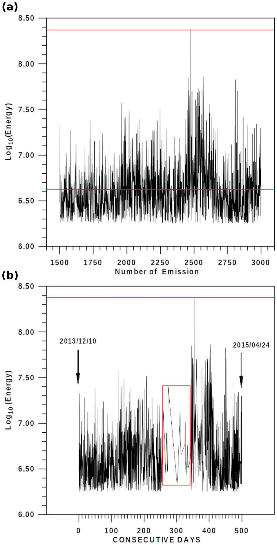
Figure 2 (a) The analyzed segment of energy emissions by means of multifractal theory, including the highest energy close to 10^8.4 J. The red line indicates the threshold value of the M_c completeness magnitude obtained from the Gutenberg–Richter law fit shown in Fig. 1. (b) The same segment of energy distributed over close to 500 consecutive days from 10 December 2013 to 24 April 2015. The largest energetic episode is highlighted with a red line. The red rectangle shows the low activity prior to the major volcanic explosion.

3 Multifractal methodology

3.1 Multifractal detrended fluctuation analysis (MF-DFA)

The examination of multifractal characteristics in nonstationary series can be addressed by utilizing the multifractal detrended fluctuation analysis (MF-DFA) technique pioneered by Talkner and Weber (2000). A comprehensive description of the MF-DFA methodology can be found in Kantelhardt et al. (2002). The MF-DFA methodology is summarized below.

We consider x_k to be a time series with a length of N, the algorithm's steps are as follows:

• (a)

  Firstly, the profile of the time series is computed as

  $$\begin{array}{}\text{(4)}& Y\left(i\right)=\sum _{k=\mathrm{1}}^i{x}_k-\langle x\rangle ,i=\mathrm{1},\mathrm{\dots },N,\end{array}$$

  where 〈x〉 is the average value of {x_k}.

• (b)

  Y(i) is divided into $N_{\mathrm{s}}=\text{int}(N/s)$ non-overlapping segments of equal length, s. Considering that length N of the series is often not a multiple of the considered segment lengths, a short part at the end of the profile would be discarded. With the aim to not disregard this part of the series, the same procedure is repeated starting from the opposite end. Consequently, 2N_s segments are obtained.

• (c)

  The local variance, F²(s,ν), is computed for each segment ν of length s using an nth-order least-square polynomial fitting to obtain the differences between “profile” segments (first step) and the corresponding polynomial fitting. The order of the polynomial is selected considering the best justified multifractal results. A fourth-order polynomial is appropriate in our case.

• (d)

  The qth-order fluctuation function is calculated by

  $$\begin{array}{}\text{(5)}& {\displaystyle }\begin{array}{rl}{\displaystyle }F(s{)}_q=& {\displaystyle }{\left[{\displaystyle \frac{\mathrm{1}}{\mathrm{2}{N}_{\mathrm{s}}}}\sum _{\mathrm{1}}^{\mathrm{2}{N}_{\mathrm{s}}}\ln \left(F^{\mathrm{2}}\right(s,\mathit{\nu }){)}^{q/\mathrm{2}}\right]}^{\mathrm{1}/qv},\\ {\displaystyle }& {\displaystyle }q\ne \mathrm{0},-\mathrm{\infty }<q<+\mathrm{\infty };\end{array}\text{(6)}& {\displaystyle }F(s{)}_{\mathrm{0}}=\left[{\displaystyle \frac{\mathrm{1}}{\mathrm{4}{N}_{\mathrm{s}}}}\sum _{\mathrm{1}}^{\mathrm{2}{N}_{\mathrm{s}}}\ln \left(F^{\mathrm{2}}\right(s,\mathit{\nu }\left)\right)\right],q=\mathrm{0}.\end{array}$$

  The steps (b), (c), and (d) must be repeated for several scales s, with it being appropriate that these scales vary within the range (m+2, $N/\mathrm{4}$), where m=4 is the chosen polynomial order (third step).

• (e)

  The qth-order fluctuation function depicts a power-law relationship concerning the segment length, s.

  $$\begin{array}{}\text{(7)}& F(s{)}_q\approx s^{h\left(q\right)}\end{array}$$

  The generalized Hurst exponent, h(q), can be determined by a linear regression of ln(F(s)_q) versus ln (s).

In the case of nonstationary series, such as fractal Brownian signals, the exponent h(q=2) will be larger than 1.0 and will satisfy $h\left(\mathrm{2}\right)=H+\mathrm{1}$, where H is the well-known Hurst exponent (Movahed and Hermanis, 2008). For stationary time series, the value h(q=2) is identical to the Hurst exponent. H>0.5 indicates persistence in long-range correlation, H≈0.5 manifests the random character of the series, and H<0.5 reflects anti-persistence. In the case of multifractal series, if positive values of q are considered, the segments ν with large variance (i.e., large deviations from the corresponding polynomial fit) will dominate the F(q(s)) average. Thus, for positive values of q, h(q) corresponds to the scaling behavior of the segments with large fluctuations. For negative values of q, each segment ν with small variance F²(s,ν) will dominate the F(q(s)) average, h(q) then describing the scaling behavior of the segments with small fluctuations (Movahed and Hermanis, 2008; Burgueño et al., 2014).

Figure 3 Six examples of multifractal spectrum. (a–d) The multifractal spectrum for four moving windows (before the highest emission). (e, f) The last two (after the highest emission) moving windows, including the extreme energy episode.

Figure 4 Evolution of parameters (a) α_max, (b) α_min, (c) α₀, and (d) Δα, describing the structure of the multifractality along the 27 moving windows. The red lines describe the smooth evolution of these parameters by means of a fifth-degree polynomial, with an r² of 0.88, 0.74, 0.72, and 0.85, respectively. The dashed line indicates MW=15, which is the window preceding the highest emission.

Figure 5 Evolution of the (a) Hurst exponent, H(q=2); (b) asymmetry, g; and (c) complexity index, CI, of the multifractal structure. Red lines describe the smooth evolution of these parameters by means of a fifth-degree polynomial with a r²=0.85, 0.68, 0.89, respectively. The dashed line indicates MW=15, which is the window that precedes the highest emission.

3.2 The singularity spectrum

The singularity spectrum, f(α), is related to the generalized Hurst exponent, h(q), through of the Legendre transform (Kantelhardt et al., 2002). This relationship is articulated as follows:

$$\begin{array}{}\text{(8)}& {\displaystyle }\begin{array}{rl}{\displaystyle }\mathit{\alpha }=h\left(q\right)+q{\displaystyle \frac{\mathrm{d}h\left(q\right)}{\mathrm{d}q}}\leftarrow & {\displaystyle }\text{Legendre\hspace{0.17em}\hspace{0.17em}transform}\to \\ {\displaystyle }& {\displaystyle }f\left(\mathit{\alpha }\right)=q\mathit{\{}\mathit{\alpha }-h(q\left)\mathit{\right\}}+\mathrm{1},\end{array}\end{array}$$

where α is the Hölder exponent, which is used to study the scaling properties and the distribution of singularities. Each value of α corresponds to a different type of singularity, and the function of these exponents, known as the singularity spectrum, f(α), describes the fractal dimension of the sets of points sharing the same Hölder exponent (Frisch and Parisi, 1985; Lux, 2004). The multifractal scaling exponent is also known as the mass exponent:

$$\begin{array}{}\text{(9)}& \mathit{\tau }\left(q\right)=qh\left(q\right)-\mathrm{1},\end{array}$$

and the Hölder exponent is defined as

$$\begin{array}{}\text{(10)}& \mathit{\alpha }\left(q\right)=\mathrm{d}\mathit{\tau }\left(q\right)/\mathrm{d}q.\end{array}$$

The function f(α) describes the subset dimension of the series characterized by the same singularity strength, α, with the singularity strength with maximum spectrum denoted by α₀. Small values of α₀ mean that the underlying process loses fine-structure – that is, becomes more regular in appearance; conversely, a large value of α₀ ensures higher complexity. The shape of f(α) may be fitted to a quadratic function around the position α₀:

$$\begin{array}{}\text{(11)}& f\left(\mathit{\alpha }\right)=A(\mathit{\alpha }-{\mathit{\alpha }}_{\mathrm{0}}{)}^{\mathrm{2}}+B(\mathit{\alpha }-{\mathit{\alpha }}_{\mathrm{0}})+C.\end{array}$$

The coefficient B shows the asymmetry of the spectrum, being null for a symmetric spectrum. A right-skewed spectrum, B>0, indicates a fine structure, while left-skewed shapes, B<0, point to a smooth structure. The width of the spectrum, W, can be obtained by extrapolating the fitted curve f(α) to zero or, in other words, extrapolating the multifractal spectrum to $q\to \pm \mathrm{\infty }$. The spectral amplitude is defined as

$$\begin{array}{}\text{(12)}& W={\mathit{\alpha }}_{\text{max}}-{\mathit{\alpha }}_{\text{min}},\end{array}$$

with $f\left({\mathit{\alpha }}_{\text{max}}\right)=f\left({\mathit{\alpha }}_{\text{min}}\right)=\mathrm{0}$ and ${\mathit{\alpha }}_{\text{max}}(q\to -\mathrm{\infty })$ being larger than ${\mathit{\alpha }}_{\text{min}}(q\to +\mathrm{\infty })$. Given that q needs to be chosen many times, ranging, for instance, within the (−15, +15) interval, α_max and α_min are obtained by numerically extrapolating Eq. (11) for f(α)=0.

The multifractal parameters used to detect the evolution towards an extreme energy emission are the central Hölder α₀ and the extreme Hölder exponents, α_max and α_min, respectively, accomplishing f(a₀)=1.0 and $f\left({\mathit{\alpha }}_{\text{max}}\right)=f\left({\mathit{\alpha }}_{\text{min}}\right)=\mathrm{0}$. The multi-spectral amplitude W (Eq. 12) and the multifractal asymmetry, γ, also contribute to detecting the proximity to an extreme emission.

$$\begin{array}{}\text{(13)}& \mathit{\gamma }={\displaystyle \frac{{\mathit{\alpha }}_{\text{max}}-{\mathit{\alpha }}_{\mathrm{0}}}{{\mathit{\alpha }}_{\mathrm{0}}-{\mathit{\alpha }}_{\text{min}}}}\end{array}$$

All these parameters are combined in a single complexity index, CI, defined in Shimizu et al. (2002) as

$$\begin{array}{}\text{(14)}& \mathrm{\text{CI}}\left(j\right)=\left[{\displaystyle \frac{{\mathit{\alpha }}_{\mathrm{0}}\left(j\right)-\langle {\mathit{\alpha }}_{\mathrm{0}}\rangle }{\mathit{\sigma }\left({\mathit{\alpha }}_{\mathrm{0}}\right)}}\right]+\left[{\displaystyle \frac{W_j-\langle W\rangle }{\mathit{\sigma }\left(W\right)}}\right]+\left[{\displaystyle \frac{{\mathit{\gamma }}_j-\langle \mathit{\gamma }\rangle }{\mathit{\sigma }\left(\mathit{\gamma }\right)}}\right],\end{array}$$

with $j=\mathrm{1},\mathrm{\dots },N$ representing the N data segments for which the multifractal spectrum is computed and 〈*〉 and σ(*), the corresponding average and standard deviation per each parameter, calculated in the N samples. The evolution of every multifractal parameter close to the extreme emission of energy will be clearly decreasing or increasing depending on every one of the specific parameters (α₀, α_max, α_min, W, and γ), which will then affect the global CI.

4 Results

4.1 Evolution of the multifractal parameters

The evolution of the multifractal parameters is analyzed by applying the multifractal detrended fluctuation analysis algorithm (MF-DFA) to 27 moving window (MW) data of 1000 elements in length (sufficient to obtain accurate multifractal analyses, manifested by the obtained evolution of the Hölder exponent, the generalized Hurst exponent, and a well-obtained multifractal spectrum) and shift of 100 elements in length. In this way, the multifractal structure is analyzed from the beginning of the available data series up to a notable number of volcanic energy emissions after the onset of extreme energy, E, which is close to log ₁₀E=8.4. A first point of view of the evolution of the multifractal structure is depicted in Fig. 3, where neither the first four moving windows (before the highest emission) nor the final two (after the highest emission) include the emission of the mentioned extreme energy. A simple review of the multifractal structure is not sufficient to detect the proximity to the highest emission given that a good fit of the empiric values of multifractality to a theoretical second-degree polynomial structure does not imply vicinity to an extreme maximum emission. Nevertheless, the Hölder exponents, describing different multifractal amplitudes and asymmetries for every moving window suggest an alternative to detect the proximity to the highest emission.

Figure 6 Three examples of τ(q) for moving windows not including the highest emission (a–c) and three including the highest energy emission (d–f). The change in $\mathrm{d}\mathit{\tau }\left(q\right)/\mathrm{d}q$ is always detected at q=0, and the corresponding square regression coefficients of both linear evolutions are very close to 1.0.

Figure 4 describes the evolution of the Hölder parameter characteristics (α₀, α_max, α_min, W) for the 27 moving windows. Bearing in mind that the highest emission is included between MWs number 16 and 25, the most relevant results are

• (a)

  an increasing tendency of α_max, with some fluctuations before MW15 and a clear decrease after the emission of the highest energy (MW16);

• (b)

  some fluctuation in α_min up to MW16 and a fast increase after this MW;

• (c)

  a clear decrease in α₀ when arriving to MW15, with a notable increase for some of the next MWs, including in the highest emission of energy;

• (d)

  a clear maximum of W for MW16, together with evident increasing and decreasing evolutions, respectively, before and after MW16.

Additionally, Fig. 5 depicts the evolution of the Hurst exponent, h(q=2); the multifractal asymmetry, γ; and the complexity index, CI. The corresponding characteristics are

• (a)

  quite a similar structure of the Hurst exponent, h(q=2), in comparison with the evolution of α₀;

• (b)

  an evolution of the asymmetry, γ, quite similar to that of W;

• (c)

  an evolution of CI, which is also quite similar to the evolution of W.

Another possibility for the detection of the immediacy of a high-energy emission is based on the evolution of the parameter $\mathit{\tau }\left(q\right)=qh\left(q\right)-\mathrm{1}$. Figure 6 depicts six examples of MWs (the first three not including the highest emission and the other three including it). As anticipated by the mathematical theory of the multifractal algorithm, the change in $\mathrm{d}\mathit{\tau }\left(q\right)/\mathrm{d}q$ is always detected in q=0 and the corresponding square regression coefficients of both linear evolutions are very close to 1.0. Figure 7 describes the evolution of the two $\mathrm{d}\mathit{\tau }\left(q\right)/\mathrm{d}q$ values for MWs number 9 to 19, where quite an evident diminishing value of $\mathrm{d}\mathit{\tau }\left(q\right)/\mathrm{d}q$ for q>0 is noticeable up to MW16, including the moving window MW15 with the highest emission. Consequently, these results of $\mathrm{d}\mathit{\tau }\left(q\right)/\mathrm{d}q$ for q>0 also contribute to detecting the proximity to the extreme volcanic emission by means of multifractal analyses.

Figure 7 Evolution of $\mathrm{d}\mathit{\tau }/\mathrm{d}Q$ for the moving windows 9–19, with the four last MW values including the highest emission of energy of Fig. 1.

The good results obtained for the multifractal structure of volcanic emissions of Colima (Mexico) based on the fourth-order polynomials used, for instance, on cited seismology or climatology research in this document are also confirmed, bearing in mind the empirical multifractal data well fitted to the theoretical multifractal scaling exponent, τ(q), and the theoretical singularity spectrum, f(α).

4.2 Evolution of the Gutenberg–Richter b value for volcanic emissions

The results obtained by means of multifractal theory are complemented by the analysis the evolution of the b value of the Gutenberg–Richter law adapted to the volcanic emission of energy (Eq. 3), with the aim of detecting changes on this parameter along the 27 MWs.

Figure 8 Statistical values per each moving window, MW: (a) b value; (b) standard deviation; and (c) skewness of emission energy, E. The red lines represent the linear trends that correspond to MWs close to the extreme emission. The dashed lines show MW=15, which is the window preceding the highest emission.

The methodology we follow to measure the evolution of the b value in the analyzed series is as follows:

1. Determination of the magnitude of completeness (M_c). In this case, we calculate an analog of the magnitude of completeness using the entire log ₁₀E series of volcanic emissions. M_c is determined by fitting the data to Eq. (1) and calculating the coefficient of determination, ρ. The magnitude at which the coefficient of determination begins to decrease indicates the M_c. In our case, the minimum acceptable value, log ₁₀(E)=6.3, for every MW is also assumed to be the same for the whole series of volcanic emissions (Fig. 1).

2. Data collection. We gather 1000 consecutive energy emissions for each MW to ensure sufficient data for accurate analysis.

3. Calculation of the b value. Using Eq. (3), we compute the b value for each MW, considering M_c is computed in the first step. This involves considering the 1000 elements of each MW, measuring the frequency distribution of log ₁₀E, and fitting the data to Eq. (3).

4. Analysis of trends and abrupt changes. By examining b-value evolution over time, we identify any significant deviations or abrupt changes in the series, which may indicate there are underlying shifts in the energy emissions.

The evolution of the b value, together with the standard deviation and skewness of log ₁₀E for the different MWs, is represented in Fig. 8a–c. Firstly, the decreasing trend of approximately 0.27 units of b for every MW from MW11 to MW16 is notable. Additionally, it is relevant that the b values for the entire series (b=3.8; ρ=0.95), as shown in Fig. 1, and for MW16, the first moving window that includes the highest emission (b=4.2; ρ=0.96), are relatively similar. Additionally, the standard deviation of log ₁₀E corresponds to MW16 (0.27) is also remarkable and similar to that of the whole series (0.28), and a clear increment of log ₁₀E dispersion (standard deviation) is observed for the consecutive MWs approaching the extreme emission. Something similar is detected for the skewness, with a value of 1.4 (the whole series) and of 1.3 (MW16), as well as a clear increment of the skewness approaching the first MW, including the extreme volcanic energy emission. In summary, considering the b-value evolution and two basic statistical measures (standard deviation and skewness), these three factors could together further confirm the progression toward a volcanic emission of extreme energy.

Despite the practicality offered by the multifractal parameters, the Gutenberg–Richter law, and the standard deviation and skewness to detect possible forthcoming extreme emissions, the step-by-step forecasting of every emission (considering an appropriate algorithm and the results of reconstruction theory) should also be relevant to complement the control of these emissions. On the one hand, the results from this research illustrate that the evolution of various parameters clearly signals the occurrence of an extreme emission. On the other hand, a suitable forecasting algorithm could determine step by step, albeit with some level of uncertainty, the imminence of consecutive emissions. For example, an emission of log ₁₀(E)=7.52, relatively close to the extreme one, is approximately recorded 17 d before. The other three high emissions (log ₁₀(E)=7.84, 7.71, and 7.65) are detected just a day or a few hours before the cited extreme emission. Remembering the foreshock concept in seismology, these four high emissions could be the “foreshocks” of the expected extreme emission. Nevertheless, whereas the first cited high emission, log ₁₀(E)=7.52, could be a warning 17 d before the extreme emission, the other three high emissions are detected only a few hours before the extreme episode. Conversely, the warning parameters proposed in this study detect signs of a forthcoming extreme energy emission a notable number of days before. A good example is the evolution of the complexity index, CI, which clearly increases from MW6 to MW11 (interval close to 100 d) and oscillates from MW12 to MW15 (close to 90 d before the extreme emission).

5 Conclusions

The analysis of the complexity and possible forecasting of potentially damaging volcanic emissions of energy, previously conducted from the point of view of the reconstruction theorem, have now been conducted in this study by means of the multifractal theory, with additional proxies based on the evolution of the b value, and two basic statistical measures (standard deviation and skewness). The obtained results enable a deeper comprehension of the intricate physical mechanisms that govern these geophysical phenomena. It is essential not to overlook the significance of the nowcasting, rooted in statistics; forecasting algorithms, which rely on predictive models; and reconstruction theorem. It is crucial to recall that the primary aim of this research is not to provide precise forecasts for every volcanic energy emission. It rather focuses on identifying the most indicative parameters that exhibit trends suggestive of a potential onset of extreme energy emissions. In summary, the integration of the multifractal structure theory, basic statistical parameters, and the Gutenberg–Richter law across a series of moving windows, together with the basis given by the reconstruction theorem, holds promise for significantly enhancing the predictability of high volcanic energy emissions over extended time intervals. Such advancements can help in preventively mitigating the effects of these volcanic emissions.