the Creative Commons Attribution 4.0 License.
the Creative Commons Attribution 4.0 License.
 | 13 Mar 2024
Phytoplankton retention mechanisms in estuaries: a case study of the Elbe estuary
Laurin Steidle
Ross Vennell
Due to their role as primary producers, phytoplankton are essential to the productivity of estuarine ecosystems. However, it is important to understand how these nearly passive organisms are able to persist within estuaries when river inflow results in a net outflow to the ocean. Estuaries also represent challenging habitats due to a strong salinity gradient. Little is known about how phytoplankton are able to be retained within estuaries. We present a new individual-based Lagrangian model of the Elbe estuary which examines possible retention mechanisms for phytoplankton. Specifically, we investigated how reproduction, sinking and rising, and diel vertical migration may allow populations to persist within the estuary. We find that vertical migration, especially rising, favors retention, while fast sinking does not. We further provide first estimates of outwashing losses. Our simulations illustrate that riverbanks and tidal flats are essential for the long-term survival of phytoplankton populations, as they provide refuges from strong downstream currents. These results contribute to the understanding needed to advance the ecosystem-based management of estuaries.
- Article
(3381 KB) - Full-text XML
- BibTeX
- EndNote


Estuaries are highly productive ecosystems. Their relatively small area disproportionally contributes to the global carbon cycle, along with their roles as a source of nutrients and hatching grounds for marine ecosystems (Cloern et al., 2014; Arevalo et al., 2023). Estuaries are of great importance for anthropogenic use, which also exposes them to many stressors such as diking, dredging and fishing (Jennerjahn and Mitchell, 2013; Brown et al., 2022; Wilson, 2002). Estuaries present challenging dynamics to their smallest residents due to their strong salinity gradient and net transport to the ocean. Here, we explore how phytoplankton, drifting small primary producers that form the basis of estuarine food webs, can persist within such dynamic environments.
Like most ecosystems, estuarine ecosystem dynamics are strongly controlled by primary producers, in particular phytoplankton (Chen et al., 2023). Apart from biofilm-forming phytoplankton, which are attached to their substrate (Cheah and Chan, 2022), the vast majority of phytoplankton organisms drift passively in currents, though they may be able to influence their vertical movement. With the estuary having a net outwards flow, we would expect phytoplankton to move downstream over time and to be washed out from limnic waters into marine waters via brackish waters. Hence, the question of how phytoplankton, the drifting base of estuarine food webs, are able to maintain their population size without declining due to the net transport into the open ocean arises. If we assume that the population is not exclusively maintained by a self-maintaining source population upstream that is washed into the estuary, then there must be some sort of retention mechanism that enables the phytoplankton population to persist within the estuary.
There are different theories about how estuarine phytoplankton populations are able to maintain their position. Previous observational studies suggested several possible mechanisms that could enable the retention of phytoplankton populations within estuarine systems: vertical migration – in the form of sinking, rising, or diel migration – and stickiness.
Diel vertical migration is a process where organisms move up and down in the water column in response to the sun. This movement may favor retention by allowing plankton to reduce the time they spend in the faster downstream currents at the water surface. A study by Anderson and Stolzenbach (1985) showed that diel-migrating dinoflagellates were able to outcompete other non-motile phytoplankton in an embayment environment and even compensate for outwashing losses through reproduction, increasing their abundance. However, this also implies that the growing part of the population is somehow retaining their position. If the regrowing population is also continuously drifting downstream it will not be able to sustain itself in that area and will ultimately die out due to unfavorable salinity conditions in marine waters (Admiraal, 1976; von Alvensleben et al., 2016; Jiang et al., 2020). The presence of diel migration has mostly been demonstrated for motile phytoplankton such as dinoflagellates (Hall et al., 2015; Crawford and Purdie, 1991; Hall and Paerl, 2011) and zooplankton species (Kimmerer et al., 2002). While the motivation for diel migration differs for autotrophs, mixotrophs, and heterotrophs, the consequence remains the same: an upward movement during the day and a downward movement during the night.
Estuaries are complex and strongly dynamic systems, such that it is still difficult to predict their ecosystem dynamics or the effects of anthropogenic impacts due to their complex bathymetry (MacWilliams et al., 2016; Fringer et al., 2019). Nevertheless, there are sophisticated estuarine models that are able to reproduce the complex dynamics of estuaries reasonably well. This includes currents and water levels on the physical side but also chlorophyll concentrations and other biologically driven properties (Pein et al., 2021; Schöl et al., 2014). However, these are Eulerian models. This means that they are based on a fixed grid and calculate the concentration of a tracer, such as phytoplankton, at each grid cell. This makes it difficult to study concepts such as retention times, as they lack temporal consistency, meaning that the life history and trajectory of a phytoplankton cell cannot be tracked. Previous modeling studies have attempted to overcome this problem using a Lagrangian approach. A Lagrangian model does not try to track, e.g., concentrations at fixed positions but rather follows the motion of individual particles that can be used to represent, e.g., water parcels or organisms. Their ability to resolve the interactions of individual phytoplankton cells or aggregates with the bathymetry (e.g., through settling or stranding) while maintaining temporal consistency is essential for investigating retention mechanisms.
Simons et al. (2006) and Kimmerer et al. (2014) used a Lagrangian model to study zooplankton retention. Simons et al. (2006) examined the dispersal and flushing times of mussel larvae in the St. Lawrence estuary, while Kimmerer et al. (2014) examined zooplankton movement in the San Francisco estuary. They were able to show that sinking and diel vertical migration slow the outwashing process and might be a beneficial retention strategy. However, they did so by ignoring key processes like reproduction, mortality, stranding, and sedimentation processes. Moreover, both studies were based on low-resolution structured grid models, which, we suspect, under-represent the complex bathymetry of estuarine systems (Ye et al., 2018).
Diatoms or benthic microalgae in particular have been observed to be strongly negatively buoyant and hence sink to the riverbed, remaining there for a long time (Passow, 1991; Thomas Anderson, 1998). Studies also found that phytoplankton aggregates have sticky compounds that are suspected to allow them stick to suspended particles, enabling them to sink to the riverbed or stick to their surroundings, aiding retention (Kiørboe and Hansen, 1993; van der Lee, 2000).
In summary, different retention mechanisms have been observed or examined in modeling studies. However, the observational studies were performed in isolation and major simplifications were used in the modeling studies. There is currently a lack of theoretical studies that allow for a more comprehensive overview of the interplay of vertical migration and reproduction in combination with settling and stranding as retention mechanisms.
Here, we explore possible retention mechanisms of phytoplankton, using the Elbe estuary as a case study. This is located in the north of Germany and flows into the North Sea. Like most alluvial estuaries, it is relatively shallow, with most of it averaging only a few meters in average depth. Similar to other European estuaries, it has experienced strong anthropogenic pressure over the last few centuries, most notably diking (to restrain it to a narrow channel) and dredging (to improve access to Hamburg harbor). Unlike other major European ports, the port of Hamburg is located far (roughly 100 km) from the coast. To create port access, the main channel is dredged and presents a sudden jump in bathymetry from approximately 5 m at the border of the city to up to 20 m in the port and downstream (see Fig. 1). This bathymetric jump is suspected to be the cause of a collapse in the phytoplankton population in the area, as the jump results in an increase in oxygen depletion and high ammonium remineralization downstream of the bathymetric jump (Schroeder, 1997; Holzwarth and Wirtz, 2018; Sanders et al., 2018). Ongoing dredging is carried out to maintain the depth of the navigational channel, causing high turbidity (Kappenberg and Grabemann, 2001). While important aspects of the along-channel biochemical dynamics have been studied, little is known about the vertical and shore-to-shore dynamics (Goosen et al., 1999; Dähnke et al., 2008; Sanders et al., 2018).
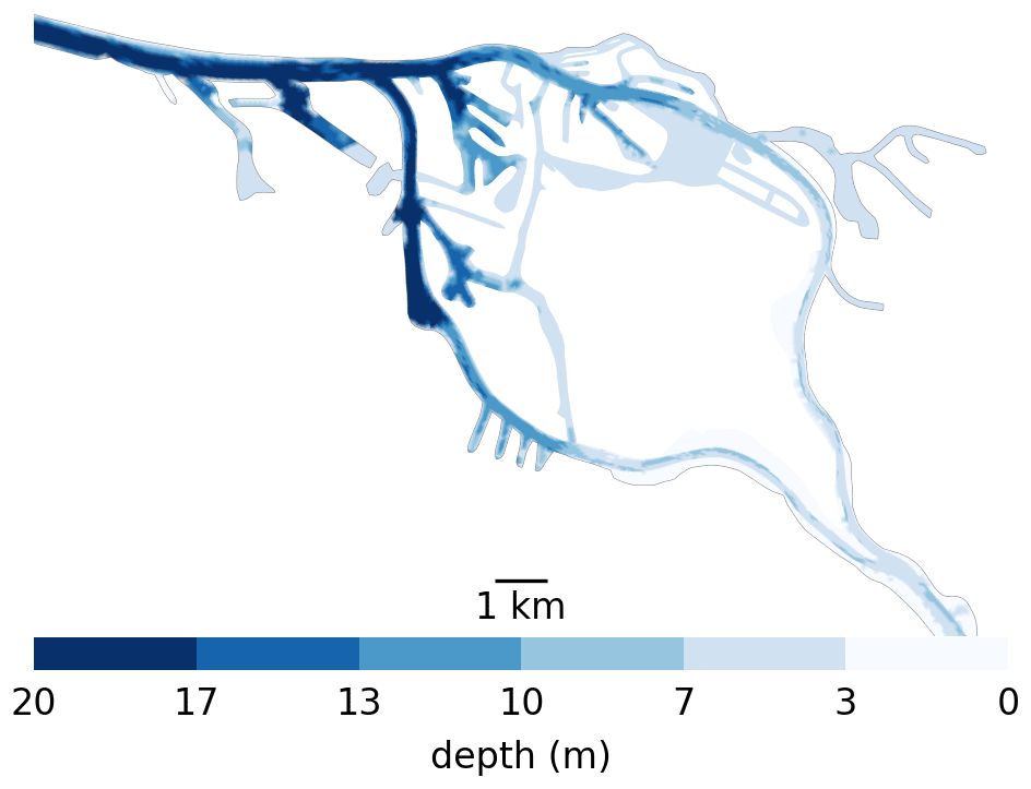
Figure 1Bathymetry used in the Elbe model around Hamburg. Note the bathymetric jumps from 5 m upstream (the right-hand side) to 10 m for a short step in the upper port area to 20 m in the lower port area all the way to the North Sea. Also note that there is only one channel to enter the harbor section of the estuary, which is 20 m deep from shore to shore. So anything that passes through has to travel through deep water.
For this purpose, we further developed the individual-based Lagrangian model OceanTracker (Vennell et al., 2021) and applied it to the Elbe estuary using the hydrodynamics calculated by a recent model, SCHISM (Pein et al., 2021). While the Lagrangian model simulated the movement of the inanimate organisms, we included key phytoplankton features such as reproduction and mortality, sinking and rising, and diel vertical migration. Using this model, we investigate the conditions under which phytoplankton retention can be reproduced.
2.1 Model description
In our study we use a Lagrangian approach with the particle tracking model OceanTracker (Vennell et al., 2021). While off-line particle tracking on unstructured grids has been relatively computationally expensive until recently (Vennell et al., 2021), it offers several advantages. Firstly, it allows us to reuse computationally expensive hydrodynamic models to model tracer-like objects. This is much faster overall than recalculating the advection–diffusion equation in an Eularian model. Secondly, because we are simulating individually particles, we are able to observe their tracks. In our model, we use these particles to represent phytoplankton cells. Alternatively, these particles could also be interpreted as aggregates colonized by phytoplankton. The temporal consistency of a Lagrangian model – the fact that we know the history of each particle – makes the interpretation of our results more intuitive and allows us to include individual-based properties and processes that cannot be represented in Eulerian models, e.g., retention times.
We use the hydrodynamic data generated by the latest SCHISM model of the Elbe estuary (Pein et al., 2021) from the weir at Geesthacht to the North Sea, including several side channels and the port area (see Fig. 2). SCHISM solves the Reynolds-averaged Navier–Stokes equations on unstructured meshes, assuming hydrostatic conditions and using a time step of 60 s. The unstructured mesh is three-dimensional and consists of 32 000 horizontal nodes that use terrain-following coordinates based on the LSC2 technique (Zhang et al., 2016) for the vertical grid, allowing a maximum of 20 levels. Regions with depths of less than 2 m are resolved using only one vertical level. Bathymetric data were provided by the German Federal Maritime and Hydrographic Agency (Bundesamt für Seeschifffahrt und Hydrographie, BSH) and the German Waterways Agency (Wasserstraßen- und Schifffahrtsamt, WSA) and have a horizontal resolution of 50 m in the German Bight, 10 m in the Elbe estuary, and 5 m in Hamburg port (Stanev et al., 2019). The boundary conditions on the seaward side include the sea surface elevation, horizontal currents, salinity, and temperature (Stanev et al., 2019), and those on the landward side include the discharge and temperature of the Elbe River. Atmospheric forcing includes wind, air temperature, precipitation, and shortwave and longwave radiation (Stanev et al., 2019). Model validation is based on tide gauge stations and long-term stationary measurements of salinity, water temperature, and horizontal currents. Biochemical variables, including chlorophyll, are based on long-term measurements at the Seemannshöft and Grauerort stations (Pein et al., 2021). The model provides us with a node-based mesh containing a range of information such as water velocity, salinity, water level, and dispersion. The year represented by that dataset is 2012. The temporal resolution of the dataset is 1 h, and it has dynamically varying spatial resolution, with the distance between nodes ranging from 5 to 1400 m (the median distance is approximately 75 m).
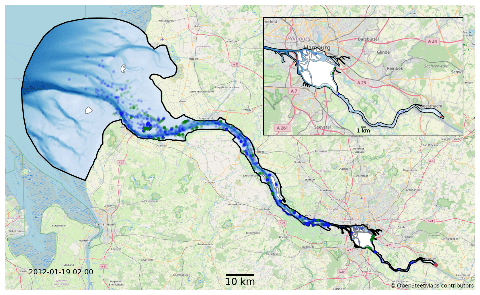
Figure 2Map of the full model domain, with Geesthacht representing the upstream border on the right and the North Sea representing the downstream border on the left. The black outline marks the edge of the model domain. Blue and green dots indicate snapshots of the status of a fraction of the phytoplankton in the model. The location of the initial release is shown in red. Blue represents floating phytoplankton; green represents phytoplankton stranded by the receding tide. The background map was provided © OpenStreetMap contributors 2023. Distributed under the Open Data Commons Open Database License (ODbL) v1.0.
We give a set of biological features to the otherwise inanimate organisms. These features include reproduction and mortality, vertical movement in the form of sinking, rising, or diel vertical migration, stranding, and settling on the riverbed.
Reproduction is represented as a fission process where each phytoplankton cell has a probability of splitting, effectively producing a copy. This is a novel feature applied in OceanTracker that has not been included in any previous Lagrangian model of this type. OceanTracker's recent advances in computational efficiency (Vennell et al., 2021) and buffer handling make it possible to simulate a large number of particles over a long period of time on unstructured grids for the first time. We perform multiple simulations for a range of reproduction rates, implemented as fission probabilities evaluated every minute, that are constant over the lifetime of the cell. While a fixed reproduction rate is a simplification that does not allow for more realistic simulation of the population dynamics of a particular species, it does allow us to investigate the general mechanisms that enable plankton retention.
Mortality is induced by one of three processes: high salinity, drying out while stranded, or long-term light limitation. When particle cells are exposed to high-salinity water (above 20 PSU), a mortality probability of 0.5 % min−1 is applied, with dead phytoplankton cells removed from the simulation (see the salinity map in Fig. C1). This threshold was chosen based on the range of salinity tolerances of the estuarine phytoplankton species presented in von Alvensleben et al. (2016). This is only an approximation, and the salinity tolerances of many estuarine phytoplankton species deviate from this. However, the main motivation for this choice is that most of the phytoplankton cells that die through this process have been beyond the isohaline for more than 12 h (one tidal cycle), after which it is assumed that they will not return through this isohaline. Anything outside the 20 PSU isohaline is not considered part of the estuary for the purposes of this study. Therefore, we are not tailoring our salinity tolerance to a specific species but rather testing whether they can persist within this isohaline. We consider phytoplankton cells that were stranded out of the water by the receding tide and have lain dry for more than 7 consecutive days to be dead and remove them. Note that these dry cells are not typically devoid of water, but they are considered “dry” if the majority of their area has a water level below 0.1 m. Additionally, in nature, these areas typically contain small sub-resolution structures such as tidal ripples or small puddles and vegetation that allows these areas to remain wet for periods longer than one tidal cycle. There are currently no studies investigating the time range for the survival of phytoplankton stranded on tidal flats or marshes in estuaries. Therefore, we performed a sensitivity analysis to determine the effect of this parameter on the retention success of the phytoplankton population (see Appendix A). Phytoplankton cells will also die if they are light limited for 14 d. This value is based on measurements presented in Walter et al. (2017) which imply that the majority of the phytoplankton are dead after 14 d of light limitation. A sensitivity analysis for this parameter is presented in Appendix B. They are considered light limited below a depth of 1 m, as estimated with the Beer–Lambert law using SPM data presented in Stanev et al. (2019). The initial batch of phytoplankton cells start their life with a full light budget of 14 d, and each minute below 1 m reduces this budget by 1 min, while the opposite applies if the cells are above 1 m. When a cell splits, both inherit the same remaining light budget.
We investigate the effects of different patterns of vertical motion. The first is monodirectional upward or downward vertical motion, representing either positively or negatively buoyant phytoplankton. This buoyancy can be interpreted as either being due to the active choice of buoyancy by the organism through adaptation or being governed by the suspended matter aggregate on which it lives. For monodirectional vertical motion, we assign each phytoplankton cell a vertical velocity which remains constant throughout its lifetime. The second mode of vertical motion is diel vertical migration. Here, phytoplankton cells change their direction of motion based on the current phase of the sun, creating a motion pattern where they rise during the day and sink during the night. This behavior is often assumed to be performed to maximize light capture while avoiding predation – or, as we suspect, to increase retention.
We include a settling and resuspension model to represent tidal stranding and phytoplankton cells settling on the bed of the estuary. Stranded phytoplankton and microphytobenthos have been shown on several occasions to be a major driver of estuarine primary production (Carlson et al., 1984; De Jonge and Van Beuselom, 1992; Kromkamp et al., 1995; Savelli et al., 2019). Phytoplankton cells become stranded when the current grid cell becomes dry, and they stay in place until they are resuspended or dry out. They are not allowed to move from wet cells to dry cells by the random walk diffusion applied to all phytoplankton cells. A grid cell is considered “dry” based on the flag it is given in the SCHISM hydrodynamic model output. Once this grid cell is flooded again, all the stranded phytoplankton cells are resuspended and able to move again. Phytoplankton cells settle on the bed once they attempt to move below the model's bottom boundary, and they are resuspended based on a critical sheer velocity of 0.009 m s−1. The velocity profile in the bottom layer, or log layer, is calculated by
where U is the friction velocity (representing the drag at height z above the seabed), κ is the von Kármán constant, z0 is a length scale reflecting the bottom roughness, and u* is the critical friction velocity. If the friction velocity is above the critical friction velocity, the phytoplankton cell is resuspended. Phytoplankton cells that are stranded or have settled on the bed are allowed to reproduce. Phytoplankton cells are not only advected but also diffused based on eddy diffusivity, which is crucial to represent tidal-pumping processes. Diffusion is modeled using a random walk obtained using a random number generator with a normal distribution. Horizontally, the standard distribution of the random walk is set to 0.1 m s−1. The vertical displacement of a phytoplankton cell ∂zi is calculated by
based on Yamazaki et al. (2014), where zi is the vertical position of the phytoplankton cell, is the vertical eddy diffusivity gradient, Kv is the vertical eddy diffusivity, and N is the normal distribution. The term is needed to avoid phytoplankton accumulation at the top and bottom of the water column in the hydrodynamic model output.
For each phytoplankton cell, we log their distance traveled, age, water depth, and status (whether they are drifting or have settled on the river bank or bottom). This allows us to, for example, compare a successfully retained phytoplankton cell (older than 3 months) with an unsuccessfully retained phytoplankton cell (dead after less than 3 months). These observables are recorded every 12 h starting at midnight.
Model simulations and visualizations are performed in Python, making heavy use of Numba, a LLVM-based Python JIT compiler (Lam et al., 2015), to significantly speed up the simulations (Vennell et al., 2021). Trajectories are calculated using a second-order Runge–Kutta scheme with a fixed time step of 60 s. Flow velocities, like all other hydrodynamic data, are interpolated linearly in time and linearly in space on the vertical axis and on the horizontal axis using barycentric coordinates, with the exception of water velocity in the bottom cell, where logarithmic vertical interpolation is used to represent drag forces more accurately.
2.2 Experimental configurations
We perform two sets of experiments to test the influences of different vertical movements on the retention success of phytoplankton in the Elbe estuary.
In the first experiment, we examine a range of different monodirectional upward or downward particle velocities from −10 to +10 mm s−1 in 2 mm s−1 steps, which represent sinking or rising phytoplankton organisms (Fennessy and Dyer, 1996). Each vertical velocity is examined for a range of different reproduction rates expressed as population doubling times ranging from 40 to 404 d with logarithmic scaling. In the following, we use “reproduction rate” to refer to the prescribed population growth rate under idealized conditions and “growth rate” whenever we describe the population growth in nature. The prescribed population growth rate can be interpreted as the potential average net doubling time in the presence of predation, mortality, and nutrient availability when testing the effect of outwashing. In the second set of model experiments, we study the influences of possible diel vertical migration patterns for the same vertical velocities and reproduction rates. Hence, a total of 187 different scenarios are tested.
In both sets of experiments, we release 10 000 individuals representing a subset of the the studied phytoplankton population at the beginning of the year. This results in over 1 billion individual particles being simulated for each case, with approximately 1 million simultaneously active particles counted over all cases for a total of 500 000 time steps. This corresponds to an approximately 1:1 ratio of simulated phytoplankton cells to mesh nodes in the hydrodynamic model at each time step. The initial population is homogeneously distributed in a volume covering the full water column at the weir in Geesthacht (see Fig. 2), and we examine how the population distributes itself over the estuary and whether it is able to maintain its population size over time. Conceptually, we consider a population to be successfully retained if it is able to sustain itself over the long term or even shows growth. Practically, this is evaluated by comparing the population size at the end of the year to the size after release. The choice of 1 year is considered reasonable because it covers the full seasonal cycle and is also much longer than the average exit or flushing time of the estuary (see Fig. 6). The first 3 months of the simulations are considered an initial model spin-up time during which the initial population is dispersed downstream throughout the estuary. Population size changes are measured at the end of the year relative to the population size after this initial spin-up time.
Computations were performed on the supercomputer Mistral at the German Climate Computing Center (DKRZ) in Hamburg, Germany. The simulations were performed on a compute node with two Intel Xeon E5-2680 v3 12-core processors (Haswell) and 128 GB of RAM for a total run time of approximately 4.5 h.
3.1 Retention success in different scenarios
The results of the retention experiments are visualized as heatmaps in Fig. 3. Figure 3a shows the results for the monodirectional vertical migration scenarios, i.e., constant sinking or rising. Figure 3b shows the results for the diel vertical migration scenarios. Each pixel in the heatmap represents a simulation with a specific combination of vertical velocity and reproduction rate expressed as a population doubling time. The color indicates the relative population change after 1 year. White pixels and the boundary between green and brown pixels represent net-zero growth rate simulations. In this case, the losses are equal to the growth. Therefore, we can use the reproduction rate as an estimate for the total relative losses due to downstream transport, drying out while being stranded, and light starvation.
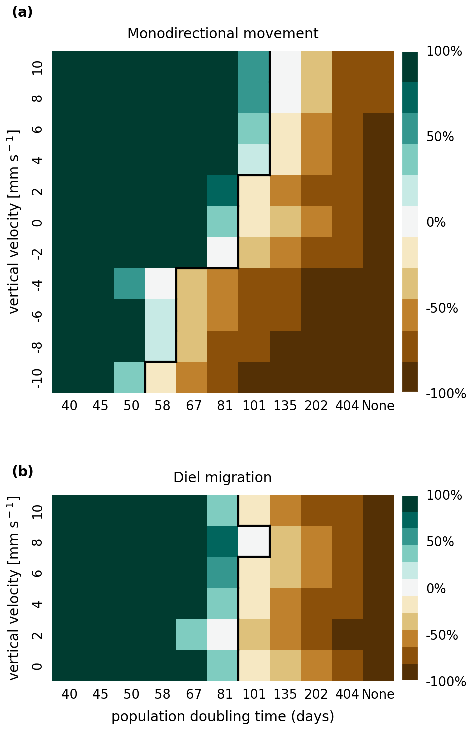
Figure 3Relative population changes for the monodirectional movement (a) and diel migration (b) scenarios. Positive vertical velocities indicate an upwards drift. Positive population changes represent a retention success (green), while negative population changes represent an eventual total loss of the population (brown). The vertical black lines indicate the boundary between the successfully and unsuccessfully retained scenarios.
Our simulations show that the population is able to successfully persist under certain conditions. Passively drifting phytoplankton are able to sustain themselves in the estuary if they have a reproduction rate that doubles their population size within approximately 3 months (see Fig. 3). Note that the growth rates realized in nature may vary from this value due to, e.g., nutrient or temperature limitations. The reproduction thresholds should be interpreted as an upper bound rather than an accurate estimate of the growth rate.
For the case of monodirectional movement, we see that a higher positive velocity (representing buoyancy) and higher reproduction rates are more beneficial for retention success than a downward-oriented velocity (sinking) and lower reproduction rates. As expected, simulations in which the reproduction is set to zero do not show any retention success. While it is easy to understand that high reproduction rates aid retention, we were surprised that buoyant phytoplankton cells are more successful at maintaining their growth in an estuary than sinking ones.
For the case of diel vertical migration in the velocity range of 4 to 10 mm s−1, we see equal or higher retention success compared to the case with no vertical migration. A diel velocity of 2 mm s−1 is less successful than no migration. Most importantly, none of the diel migration scenarios improve the retention success when compared to passively drifting organisms.
3.2 Spatial factors
We now take a closer look at spatial factors that allow phytoplankton cells to maintain net growth in the estuary. For this analysis, we used data from both sets of experiments, i.e., from all cases. Figure 4 compares two box plots of the average water depth at the location of each phytoplankton cell: the first box plot is for those cells that remained alive for less than 3 months (short living) and the second is for those cells that remained alive for more than 3 months (long living). Depth is measured relative to the current water surface. Therefore, a value greater than zero indicates that the phytoplankton cell is stranded on the shore during an ebb tide. For reference, the water level varies on average by about 5 m due to the tides (Stanev et al., 2019; Schöl et al., 2014). These analyses show that long-living phytoplankton predominantly live close to the river banks in shallower waters or on tidal flats.
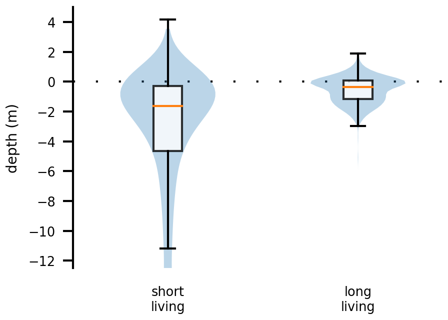
Figure 4Box and violin plots showing vertical distributions of phytoplankton that are passively drifting. The plot labeled “short living” is for the phytoplankton younger than 3 months, and the plot labeled “long living” is for all those older than that. Depth is measured relative to the current water surface, with positive numbers indicating phytoplankton above the water surface, i.e., stranded on the shore.
Moreover, we analyze the horizontal spatial distribution of long- and short-living phytoplankton in Fig. 5. To do this, we divide the model domain into equally sized hexagons. The color of each hexagon indicates the average age of the phytoplankton cells within it, calculated across all cases. Note that the spatial age structure is similar for all cases. Hexagons with a yellow color indicate an average age of over 3 months. These yellow areas are mainly found along the river banks in shallow waters or tidal flats.
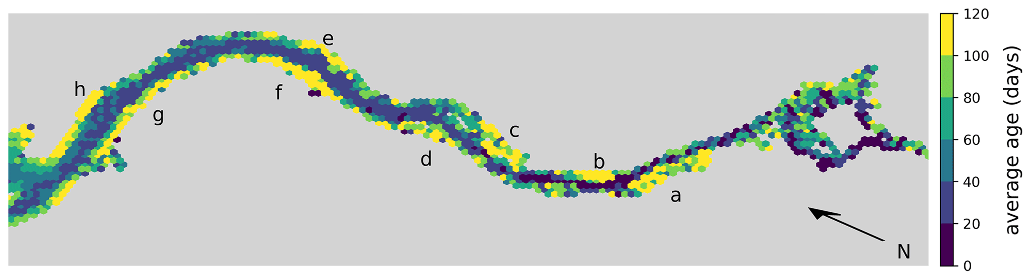
Figure 5Hex-bin heatmap of the average age of phytoplankton cells in the Elbe estuary across all cases. Hamburg's port area is located on the right, with the North Sea to the left. Colors indicate the age of the phytoplankton, with yellowish colors indicating an average age of over 3 months. Yellow areas are mainly found along the river banks in shallow waters or tidal flats. The important areas are Mühlenberger Loch (a), Wedeler Marsch (b), Haseldorfer Binnenelbe (c), Asseler- and Schwarztonnensand (d), at the mouths of the Stör (e) and Wischhafener Süderelbe (f), and at Nordkedding (g) and Neufelder Marsch (h).
For comparison, the average exit time for water parcels to reach the 20 PSU isohaline per hexagon is shown in Fig. 6. This calculation is based on a separate simulation where we released approximately 1.8 million particles that were homogeneously distributed over the estuary. We released one batch in winter during high-discharge conditions on 1 January and another batch in summer during low-discharge conditions on 1 July. Note that for this simulation, reproduction, light limitation, stranding, and settling on the riverbed were disabled to isolate the effect of advection and dispersion.
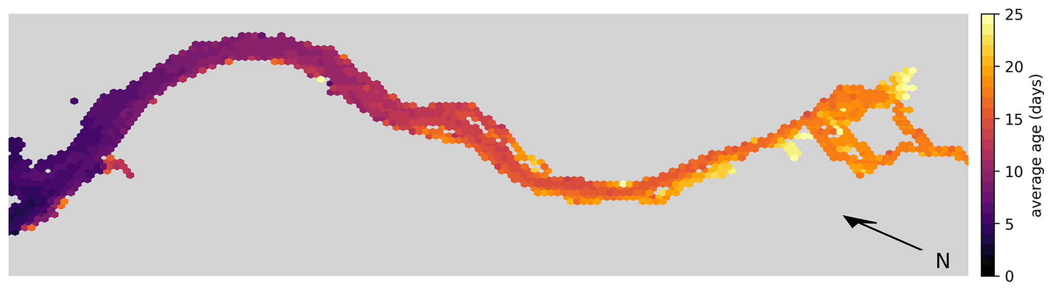
Figure 6Hex-bin heatmap showing the average exit times from the Elbe estuary (Hamburg's port area, as shown in Fig. 1, is on the right) without any reproduction, light limitation, stranding, or settling on the riverbed. The color indicates the time taken for a water parcel to reach the 20 PSU isohaline from the hexagon in which it originated.
To further investigate the reasons for the positive effect of buoyancy and the importance of shallow waters and tidal flats, we repeated the first set of simulations and disabled the reproduction of settled and stranded phytoplankton. Under these conditions, populations were unable to persist within the estuary, regardless of their vertical velocity and reproduction rate, indicating that tidal flats are essential for the survival of the population.
3.3 Interpretation and contextualization of the results
In this study, we investigated different strategies to explain how phytoplankton populations are able to maintain their population sizes in estuaries while constantly being at risk of being transported into the open ocean.
The limit on the population doubling time that we found necessary for the survival of passively drifting plankton is about 4 months (see Fig. 3). Doubling times typically realized in nature are of the order of a few days, which is 2 orders of magnitude smaller than those that we found necessary in our model (Koch et al., 2004; Wirtz, 2011). The low reproduction rates required for successful retention demonstrate that our model is also meaningful under more realistic environmental conditions, for example, if maximum growth rates cannot be reached due to nutrient or temperature limitations.
Our results suggest that shallow areas are very important for maintaining the estuary phytoplankton population. Plankton that consistently find themselves in areas that fall dry due to the tides will regularly become stranded and therefore do not move for much of the tidal cycle. We further see that positively buoyant plankton are more successful at maintaining themselves. This is probably because they are more likely to be transported high up on the river bank, where the water is less likely to reach them. This effect is emphasized in flatter regions, as the distance between the wash margin and constantly flooded areas is larger, increasing the chance of settlement or of them becoming stranded again.
Initially, we expected sinking phytoplankton to have a higher retention success than buoyant ones. However, we found that faster sinking phytoplankton are less successful at persisting. Sinking velocities of less than 2 mm s−1 are common for diatoms (Passow, 1991), while larger velocities have been observed for aggregates in the Elbe estuary (Fennessy and Dyer, 1996). Sinking phytoplankton have a reduced downstream velocity because they either settle on the riverbed, where they do not move at all, or they become close to the bed, where the average downstream velocity is lower. In addition, due to temperature-induced density stratification, the deeper water layers of the Elbe either have, on average, a lower downstream velocity than the upper water column or they move upstream (Pein et al., 2021). Nevertheless, buoyant phytoplankton showed more successful retention in our simulations. The low chance of survival in the estuary for sinking phytoplankton might be explained by light limitation in deeper waters. We expected phytoplankton to die if they are exposed to dark conditions for more than 2 weeks. Thus, sinking phytoplankton have a disadvantage compared to buoyant phytoplankton, since they are more likely to become light limited and eventually die. This suggests that dredging has a negative impact on sinking plankton because it increases both depth and turbidity (de Jonge et al., 2014), which increases the aphotic depth and therefore the volume of dark water relative to the volume of illuminated water.
We suspect that the reason for the increased retention success of diel-migrating organisms is similar to the monodirectional case. When the upwards diel migration coincides with a high tide, phytoplankton are more likely to be stranded far out on the shore, reducing their risk of being washed out quickly. The higher the upward velocities, the greater the chance of being at the waterline during high tide. However, because they are sinking for half of the day, they also tend to be light limited more frequently than positively buoyant phytoplankton. It appears that these favorable and unfavorable processes balance each other out, resulting in a similar retention success to that in the monodirectional case.
3.4 Model limitations and future perspectives
In this study, we aimed to thoroughly investigate different possible retention mechanisms in a complex Lagrangian model system with a highly resolved bathymetry. Due to this computational and spatial complexity, the biological particle properties needed to remain simple to keep computational costs manageable and interpretability high and due to a lack of high-resolution validation data.
Our model design does not resolve more complex ecosystem dynamics such as nutrient limitation and grazing by higher trophic levels. The Lagrangian model is performed offline, meaning it is not coupled to the Eulerian model that calculates the hydrodynamics and is performed after the fact. Therefore, modeling the advection and dispersal of changes in concentration fields, e.g., those of nutrients (due to growth or remineralization), was not easily possible. Future modeling efforts could couple the Lagrangian model to an Eulerian model that disperses changes in concentration fields caused by biotic activity throughout the model domain. However, this would have drastically increased both the development and computational times to a point where the study would have become infeasible in our time frame and also would have required validation data that do not exist. The key drawback of this is that growth rates could only be modeled as being constant in the current model description, similar to ad libitum experiments. This can lead to systematic errors in estimating population growth. In nature, phytoplankton growth is often limited by nutrient availability, so nutrient limitation, which slows down the growth of the population, can occur, especially in the most light-saturated areas near the shore. For this reason, we may overestimate the role of shallow areas in our model.
To be consistent with the complexity of the representation of biotic mechanisms, we use a simplistic light limitation. Phytoplankton are expected to be light limited below a water depth of 1 m and not to be light limited above this threshold. We have not included a more complex light-limitation model that takes into account current light availability and attenuation. A more realistic formulation of light limitation could particularly favor phytoplankton that exhibit diel vertical migration.
A process we mostly ignore in our study is dormancy. Our organisms can survive for 14 d in light-limited waters. However, phytoplankton species have life stages in which they can remain dormant for a long period of time and germinate again when they find themselves in more favorable waters (Thomas Anderson, 1998). In the process of choosing the light-limitation threshold, we conducted sensitivity studies testing the effect of higher light budgets. We found that light budgets of over 3 months begin to significantly increase the survivability of sinking organisms when we crudely assume that they could still reproduce under these conditions. Whether dormancy plays a significant role in an environment where the river bed is continuously dredged is unknown.
Another limitation in our modeling efforts is the lack of sub-grid-resolution structure on the shores. In our representation, we assume perfectly flat surfaces with a median distance between nodes of approximately 60 m. This “polished” model representation can lead to an underestimation of the retention success, since the surface area on which phytoplankton organisms can settle is underestimated. In nature, vegetation, rocks, or other surface irregularities provide a larger surface area on which the phytoplankton organisms can settle in moist conditions.
Our hydrodynamic dataset was limited to the year 2012. Therefore, we were not able to study different release times with the same methodology. While we do not expect the general dynamics to change, future research could examine the effect of varying the discharge throughout the seasons on retention and could address the very-long-term success (>1 year) of the population, as it is affected by inter-annual variability and climate change.
While our model does have settling and resuspension mechanics based on critical sheer velocities, we still assume a static bathymetry in which sediments are not able to move or bury phytoplankton. This masks potential losses due to phytoplankton being buried but also decreases resuspension times.
Our results clearly suggest the importance of tidal flats and shallow areas along the river banks for the persistence of primary production in the Elbe estuary. However, their effect cannot currently be quantified due to the lack of validation data. Chlorophyll data with a sufficient temporal and spatial resolution is only gathered in the center of the river. Future monitoring efforts should therefore also include data along the river shores on tidal flats or from shore to shore to quantify the effect of potential future changes caused by dredging, diking, or restoration attempts.
Frequently stranded plankton have been shown to be essential to the survival of populations in our model. However, data on their ability to survive under these conditions are scarce. Our results suggest that these conditions may be as important as their ability to quickly regrow under more favorable conditions, and we suggest that further research on plankton survivability when they are stranded is needed.
For several decades, the annual average chlorophyll concentration in the Elbe estuary has been decreasing (data available at https://www.fgg-elbe.de/elbe-datenportal.html (last access: 3 March 2024) or see Hardenbicker et al., 2014; Schöl et al., 2014), while upstream concentrations do not show this effect. The reasons for this are not fully understood, but one possible reason is the increase in dredging activity. This increases the average turbidity and thus the aphotic depth, reducing the volume of water in which phytoplankton can grow. A large fraction of the phytoplankton measured upstream of Hamburg port consists of diatoms (Muylaert and Sabbe, 1999), which typically have negative buoyancy (Passow, 1991), making them particularly susceptible to sinking in light-limited waters. Our finding that sinking phytoplankton have a harder time surviving in the estuary supports this theory.
Another mechanism that might, in part, explain the drop in phytoplankton concentration at the bathymetric jump, which has not yet been explored in our model, is the phytoplankton stickiness. Phytoplankton, especially blooming phytoplankton, have been shown to be sticky due to exudates (Kiørboe and Hansen, 1993; van der Lee, 2000; Dutz et al., 2005). Some phytoplankton also produce transparent exopolymer particles, which increase their stickiness to other particles (Windler et al., 2015; De Brouwer et al., 2005). We suspect that this, in combination with the higher turbidity induced by dredging, results in losses due to plankton aggregates sticking to negatively buoyant suspended matter and subsequently sinking to the ground, where they are starved of light. A future model study could obtain estimates of the phytoplankton losses caused by this effect.
In this study, we investigated the roles of different retention strategies for phytoplankton organisms to persist in an estuarine environment. We showed that stranding in shallow nearshore areas is essential for phytoplankton retention, and that phytoplankton that are not stranded are rapidly washed away. Our model simulations suggest that growth rates much lower than those observed in nature may be sufficient to prevent population decline due to outwashing, implying that stranding may be sufficient to maintain the population. Moreover, buoyancy and strong diel vertical migration enhance retention within the estuary. These results highlight the importance of shallow nearshore areas in maintaining the productivity of estuarine ecosystems. Our results suggest that current state-of-the-art models of estuarine ecosystems may overlook an important process, and they emphasize the need for informed ecosystem-based management to avoid the degradation of estuarine ecosystems by dredging and diking activities.
In Figs. A1 and A2, we present the results of a sensitivity analysis of stranding mortality (i.e., due to drying out) thresholds of 1 and 14 d compared to the results for 7 d shown in Fig. 3. Varying this parameter changes the breakeven point of growth and loss slightly, as expected. However, no regime shift occurs, and the observed trends remain the same.
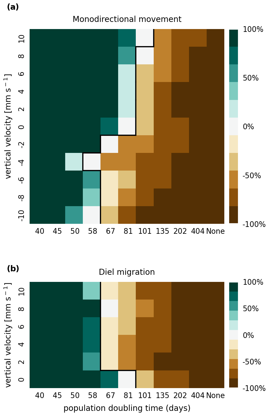
Figure A1Sensitivity analysis of mortality due to stranding (i.e., drying out) showing that the retention success obtained with a threshold of 1 d without resuspension is similar to that obtained with a threshold of 7 d before phytoplankton are culled (as shown in Fig. 3).
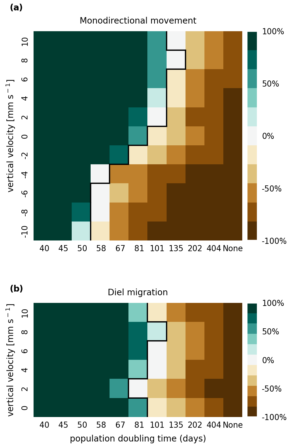
In Figs. B1 and B2, we present the results of a sensitivity analysis of mortality thresholds due to light limitation of 7 and 28 d compared to the 14 d shown in Fig. 3. Similar to the stranding mortality threshold, perturbations in this parameter change the breakeven point of growth and loss as expected. Reducing the tolerated light deficit to half that observed in laboratory studies (Walter et al., 2017) has a particularly pronounced effect on sinking phytoplankton cells, which are more frequently light limited. This is most clearly visible in the −10 mm case, which shows that the breakeven point is reached at a doubling time of below 40 d. Nevertheless, the trends discussed, e.g., breakeven points at doubling times that are much larger then those observed in nature, the favoring of buoyant cells over sinking cells, and the importance of shallow areas, remain the same.
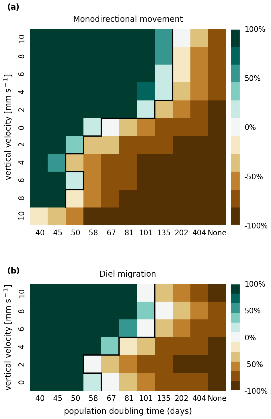
Figure B1Sensitivity analysis of mortality due to light limitation showing that the retention success obtained with a light deficit threshold of 7 d is similar to that obtained with a threshold of 14 d before phytoplankton are culled (as shown in Fig. 3).
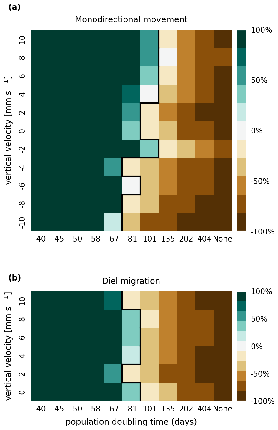
Figure C1 shows a map of average salinity of the Elbe estuary. Salinity is averaged across depths and over the whole year.
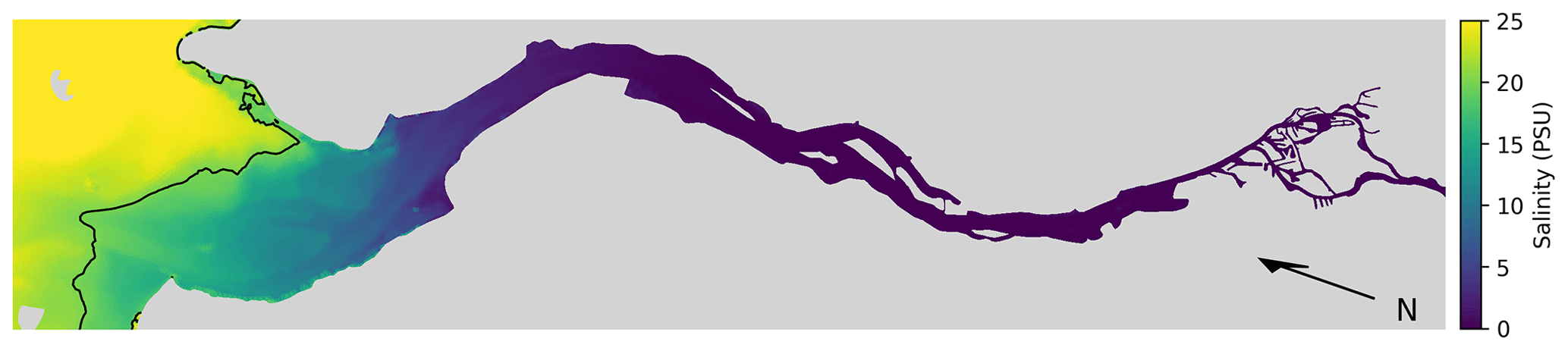
Figure C1Salinity map of the Elbe estuary, with Hamburg's port area (as shown in Fig. 1) at the bottom right. Salinity is averaged across depths and over the whole year. The 20 PSU isohaline is marked with a black line. Note that this plotted area has been extended downstream compared to Fig. 5. Also note that the color map has been capped at 25 PSU for better visibility in low-salinity areas.
Input data can be requested from Johannes Pein (johannes.pein@hereon.de). The source code, model configuration and output are available in the Zenodo repository https://doi.org/10.25592/uhhfdm.13235 (Steidle, 2023). The current version of OceanTracker is available at https://github.com/oceantracker/oceantracker (last access: 3 March 2024).
LS and RV contributed to the conception of the study. LS designed the study details and organized the hydrodynamic data. RV provided the source code for OceanTracker. RS and LS improved on the original physical model, and LS developed the biological model. LS performed the model simulations, post-processing, and visualization. LS wrote the draft of the manuscript. All authors contributed to manuscript revision and read and approved the submitted version.
The contact author has declared that neither of the authors has any competing interests.
Publisher's note: Copernicus Publications remains neutral with regard to jurisdictional claims made in the text, published maps, institutional affiliations, or any other geographical representation in this paper. While Copernicus Publications makes every effort to include appropriate place names, the final responsibility lies with the authors.
This article is part of the special issue “Turbulence and plankton”. It is not associated with a conference.
We thank Johannes Pein for providing and supporting the implementation of the hydrodynamic data, Jana Hinners for her guidance through the project, and Hans Burchard for his input on dispersion. Further, we thank Sina Remmers and Philipp Porada for providing helpful comments on the manuscript. This study was funded by the Deutsche Forschungsgemeinschaft (DFG, German Research Foundation) within Research Training Group 2530: “Biota-mediated effects on carbon cycling in estuaries” (project number 407270017), contribution to Universität Hamburg and Leibniz-Institut für Gewässerökologie und Binnenfischerei (IGB) im Forschungsverbund Berlin e.V.
This research has been supported by the Deutsche Forschungsgemeinschaft (grant no. 407270017).
This paper was edited by Enrico Calzavarini and reviewed by Elena Alekseenko and one anonymous referee.
Admiraal, W.: Salinity tolerance of benthic estuarine diatoms as tested with a rapid polarographic measurement of photosynthesis, Mar. Biol., 39, 11–18, https://doi.org/10.1007/BF00395587, 1976. a
Anderson, D. and Stolzenbach, K.: Selective retention of two dinoflagellates in a well-mixed estuarine embayment: the importance of diel vertical migration and surface avoidance, Mar. Ecol. Prog. Ser., 25, 39–50, https://doi.org/10.3354/meps025039, 1985. a
Arevalo, E., Cabral, H. N., Villeneuve, B., Possémé, C., and Lepage, M.: Fish larvae dynamics in temperate estuaries: A review on processes, patterns and factors that determine recruitment, Fish Fish., 24, 466–487, https://doi.org/10.1111/faf.12740, 2023. a
Brown, A. M., Bass, A. M., and Pickard, A. E.: Anthropogenic-estuarine interactions cause disproportionate greenhouse gas production: A review of the evidence base, Mar. Pollut. Bull., 174, 113240, https://doi.org/10.1016/j.marpolbul.2021.113240, 2022. a
Carlson, D. J., Townsend, D. W., Hilyard, A. L., and Eaton, J. F.: Effect of an intertidal mudflat on plankton of the overlying water column, Can. J. Fish. Aquat. Sci., 41, 1523–1528, https://doi.org/10.1139/f84-188, 1984. a
Cheah, Y. T. and Chan, D. J. C.: A methodological review on the characterization of microalgal biofilm and its extracellular polymeric substances, J. Appl. Microbiol., 132, 3490–3514, https://doi.org/10.1111/jam.15455, 2022. a
Chen, W., Guo, F., Huang, W., Wang, J., Zhang, M., and Wu, Q.: Advances in phytoplankton population ecology in the Pearl river estuary, Front. Environ. Sci., 11, 1–8, https://doi.org/10.3389/fenvs.2023.1084888, 2023. a
Cloern, J. E., Foster, S. Q., and Kleckner, A. E.: Phytoplankton primary production in the world's estuarine-coastal ecosystems, Biogeosciences, 11, 2477–2501, https://doi.org/10.5194/bg-11-2477-2014, 2014. a
Crawford, D. and Purdie, D.: Evidence for avoidance of flushing from an estuary by a planktonic, phototrophic ciliate, Mar. Ecol. Prog. Ser., 79, 259–265, https://doi.org/10.3354/meps079259, 1991. a
Dähnke, K., Bahlmann, E., and Emeis, K.: A nitrate sink in estuaries? An assessment by means of stable nitrate isotopes in the Elbe estuary, Limnol. Oceanogr., 53, 1504–1511, https://doi.org/10.4319/lo.2008.53.4.1504, 2008. a
De Brouwer, J. F., Wolfstein, K., Ruddy, G. K., Jones, T. E., and Stal, L. J.: Biogenic stabilization of intertidal sediments: The importance of extracellular polymeric substances produced by benthic diatoms, Microb. Ecol., 49, 501–512, https://doi.org/10.1007/s00248-004-0020-z, 2005. a
De Jonge, V. and Van Beuselom, J.: Contribution of resuspended microphytobenthos to total phytoplankton in the EMS estuary and its possible role for grazers, Neth. J. Sea Res., 30, 91–105, https://doi.org/10.1016/0077-7579(92)90049-K, 1992. a
de Jonge, V. N., Schuttelaars, H. M., van Beusekom, J. E., Talke, S. A., and de Swart, H. E.: The influence of channel deepening on estuarine turbidity levels and dynamics, as exemplified by the Ems estuary, Estuar. Coast. Shelf S., 139, 46–59, https://doi.org/10.1016/j.ecss.2013.12.030, 2014. a
Dutz, J., Klein Breteler, W., and Kramer, G.: Inhibition of copepod feeding by exudates and transparent exopolymer particles (TEP) derived from a Phaeocystis globosa dominated phytoplankton community, Harmful Algae, 4, 929–940, https://doi.org/10.1016/j.hal.2004.12.003, 2005. a
Fennessy, M. J. and Dyer, K. R.: Floc population characteristics measured with INSSEV during the Elbe estuary intercalibration experiment, J. Sea Res., 36, 55–62, https://doi.org/10.1016/s1385-1101(96)90771-6, 1996. a, b
Fringer, O. B., Dawson, C. N., He, R., Ralston, D. K., and Zhang, Y. J.: The future of coastal and estuarine modeling: Findings from a workshop, Ocean Model., 143, 101458, https://doi.org/10.1016/j.ocemod.2019.101458, 2019. a
Goosen, N. K., Kromkamp, J., Peene, J., Van Rijswijk, P., and Van Breugel, P.: Bacterial and phytoplankton production in the maximum turbidity zone of three European estuaries: The Elbe, Westerschelde and Gironde, J. Marine Syst., 22, 151–171, https://doi.org/10.1016/S0924-7963(99)00038-X, 1999. a
Hall, N. S. and Paerl, H. W.: Vertical migration patterns of phytoflagellates in relation to light and nutrient availability in a shallow microtidal estuary, Mar. Ecol. Prog. Ser., 425, 1–19, https://doi.org/10.3354/meps09031, 2011. a
Hall, N. S., Whipple, A. C., and Paerl, H. W.: Vertical spatio-temporal patterns of phytoplankton due to migration behaviors in two shallow, microtidal estuaries: Influence on phytoplankton function and structure, Estuar. Coast. Shelf S., 162, 7–21, https://doi.org/10.1016/j.ecss.2015.03.032, 2015. a
Hardenbicker, P., Rolinski, S., Weitere, M., and Fischer, H.: Contrasting long-term trends and shifts in phytoplankton dynamics in two large rivers, Int. Rev. Hydrobiol., 99, 287–299, https://doi.org/10.1002/iroh.201301680, 2014. a
Holzwarth, I. and Wirtz, K.: Anthropogenic impacts on estuarine oxygen dynamics: A model based evaluation, Estuar. Coast. Shelf S., 211, 45–61, https://doi.org/10.1016/j.ecss.2018.01.020, 2018. a
Jennerjahn, T. C. and Mitchell, S. B.: Pressures, stresses, shocks and trends in estuarine ecosystems – An introduction and synthesis, Estuar. Coast. Shelf S., 130, 1–8, https://doi.org/10.1016/j.ecss.2013.07.008, 2013. a
Jiang, L., Gerkema, T., Kromkamp, J. C., van der Wal, D., Carrasco De La Cruz, P. M., and Soetaert, K.: Drivers of the spatial phytoplankton gradient in estuarine–coastal systems: generic implications of a case study in a Dutch tidal bay, Biogeosciences, 17, 4135–4152, https://doi.org/10.5194/bg-17-4135-2020, 2020. a
Kappenberg, J. and Grabemann, I.: Variability of the mixing zones and estuarine turbidity maxima in the Elbe and Weser estuaries, Estuaries, 24, 699–706, https://doi.org/10.2307/1352878, 2001. a
Kimmerer, W. J., Burau, J. R., and Bennett, W. A.: Persistence of tidally-oriented vertical migration by zooplankton in a temperate estuary, Estuaries, 25, 359–371, https://doi.org/10.1007/BF02695979, 2002. a
Kimmerer, W. J., Gross, E. S., and MacWilliams, M. L.: Tidal migration and retention of estuarine zooplankton investigated using a particle-tracking model, Limnol. Oceanogr., 59, 901–916, https://doi.org/10.4319/lo.2014.59.3.0901, 2014. a, b
Kiørboe, T. and Hansen, J. L.: Phytoplankton aggregate formation: Observations of patterns and mechanisms of cell sticking and the significance of exopolymeric material, J. Plankton Res., 15, 993–1018, https://doi.org/10.1093/plankt/15.9.993, 1993. a, b
Koch, R. W., Guelda, D. L., and Bukaveckas, P. A.: Phytoplankton growth in the Ohio, Cumberland and Tennessee Rivers, USA: Inter-site differences in light and nutrient limitation, Aquat. Ecol., 38, 17–26, https://doi.org/10.1023/B:AECO.0000021082.42784.03, 2004. a
Kromkamp, J., Peene, J., van Rijswijk, P., Sandee, A., and Goosen, N.: Nutrients, light and primary production by phytoplankton and microphytobenthos in the eutrophic, turbid Westerschelde estuary (The Netherlands), Hydrobiologia, 311, 9–19, https://doi.org/10.1007/BF00008567, 1995. a
Lam, S. K., Pitrou, A., and Seibert, S.: Numba: A LLVM-based Python JIT Compiler, in: Proceedings of the Second Workshop on the LLVM Compiler Infrastructure in HPC, Association for Computing Machinery, New York, NY, USA, https://doi.org/10.1145/2833157.2833162, 2015. a
MacWilliams, M. L., Ateljevich, E. S., Monismith, S. G., and Enright, C.: An Overview of Multi-Dimensional Models of the Sacramento – San Joaquin Delta, San Francisco Estuary and Watershed Science, 14, 4, https://doi.org/10.15447/sfews.2016v14iss4art2, 2016. a
Muylaert, K. and Sabbe, K.: Spring phytoplankton assemblages in and around the maximum turbidity zone of the estuaries of the Elbe (Germany), the Schelde (Belgium/The Netherlands) and the Gironde (France), J. Marine Syst., 22, 133–149, https://doi.org/10.1016/S0924-7963(99)00037-8, 1999. a
Passow, U.: Species-specific sedimentation and sinking velocities of diatoms, Mar. Biol., 108, 449–455, https://doi.org/10.1007/BF01313655, 1991. a, b, c
Pein, J., Eisele, A., Sanders, T., Daewel, U., Stanev, E. V., van Beusekom, J. E. E., Staneva, J., and Schrum, C.: Seasonal Stratification and Biogeochemical Turnover in the Freshwater Reach of a Partially Mixed Dredged Estuary, Front. Mar. Sci., 8, https://doi.org/10.3389/fmars.2021.623714, 2021. a, b, c, d, e
Sanders, T., Schöl, A., and Dähnke, K.: Hot Spots of Nitrification in the Elbe Estuary and Their Impact on Nitrate Regeneration, Estuar. Coasts, 41, 128–138, https://doi.org/10.1007/s12237-017-0264-8, 2018. a, b
Savelli, R., Bertin, X., Orvain, F., Gernez, P., Dale, A., Coulombier, T., Pineau, P., Lachaussée, N., Polsenaere, P., Dupuy, C., and le Fouest, V.: Impact of Chronic and Massive Resuspension Mechanisms on the Microphytobenthos Dynamics in a Temperate Intertidal Mudflat, J. Geophys. Res.-Biogeo., 124, 3752–3777, https://doi.org/10.1029/2019JG005369, 2019. a
Schöl, A., Hein, B., Wyrwa, J., and Kirchesch, V.: Modelling Water Quality in the Elbe and its Estuary – Large Scale and Long Term Applications with Focus on the Oxygen Budget of the Estuary, Die Küste, 81, 203–232, 2014. a, b, c
Schroeder, F.: Water quality in the Elbe estuary: Significance of different processes for the oxygen deficit at Hamburg, Environ. Model. Assess., 2, 73–82, https://doi.org/10.1023/a:1019032504922, 1997. a
Simons, R. D., Monismith, S. G., Johnson, L. E., Winkler, G., and Saucier, F. J.: Zooplankton retention in the estuarine transition zone of the St. Lawrence Estuary, Limnol. Oceanogr., 51, 2621–2631, https://doi.org/10.4319/lo.2006.51.6.2621, 2006. a, b
Stanev, E. V., Jacob, B., and Pein, J.: German Bight estuaries : An inter-comparison on the basis of numerical modeling, Cont. Shelf Res., 174, 48–65, https://doi.org/10.1016/j.csr.2019.01.001, 2019. a, b, c, d, e
Steidle, L.: Phytoplankton Retention Mechanisms in Estuaries: A Case Study of the Elbe Estuary, FDM [code and data set], https://doi.org/10.25592/uhhfdm.13235, 2023. a
Thomas Anderson, J.: The effect of seasonal variability on the germination and vertical transport of a cyst forming dinoflagellate, Gyrodinium sp., in the Chesapeake Bay, Ecol. Model., 112, 85–109, https://doi.org/10.1016/S0304-3800(98)00074-X, 1998. a, b
van der Lee, W.: Parameters affecting mud floc size on a seasonal time scale: The impact of a phytoplankton bloom in the Dollard estuary, The Netherlands, in: Coastal and Estuarine Fine Sediment Processes, Elsevier, 1989, 403–421, https://doi.org/10.1016/S1568-2692(00)80134-5, 2000. a, b
Vennell, R., Scheel, M., Weppe, S., Knight, B., and Smeaton, M.: Fast lagrangian particle tracking in unstructured ocean model grids, Ocean Dynam., 71, 423–437, https://doi.org/10.1007/s10236-020-01436-7, 2021. a, b, c, d, e
von Alvensleben, N., Magnusson, M., and Heimann, K.: Salinity tolerance of four freshwater microalgal species and the effects of salinity and nutrient limitation on biochemical profiles, J. Appl. Phycol., 28, 861–876, https://doi.org/10.1007/s10811-015-0666-6, 2016. a, b
Walter, B., Peters, J., and van Beusekom, J. E.: The effect of constant darkness and short light periods on the survival and physiological fitness of two phytoplankton species and their growth potential after re-illumination, Aquat. Ecol., 51, 591–603, https://doi.org/10.1007/s10452-017-9638-z, 2017. a, b
Wilson, J. G.: Productivity, fisheries and aquaculture in temperate estuaries, Estuar. Coast. Shelf S., 55, 953–967, https://doi.org/10.1006/ecss.2002.1038, 2002. a
Windler, M., Leinweber, K., Bartulos, C. R., Philipp, B., and Kroth, P. G.: Biofilm and capsule formation of the diatom Achnanthidium minutissimum are affected by a bacterium, J. Phycol., 51, 343–355, https://doi.org/10.1111/jpy.12280, 2015. a
Wirtz, K. W.: Non-uniform scaling in phytoplankton growth rate due to intracellular light and CO2 decline, J. Plankton Res., 33, 1325–1341, https://doi.org/10.1093/plankt/fbr021, 2011. a
Yamazaki, H., Locke, C., Umlauf, L., Burchard, H., Ishimaru, T., and Kamykowski, D.: A Lagrangian model for phototaxis-induced thin layer formation, Deep-Sea Res. Pt. II, 101, 193–206, https://doi.org/10.1016/j.dsr2.2012.12.010, 2014. a
Ye, F., Zhang, Y. J., Wang, H. V., Friedrichs, M. A., Irby, I. D., Alteljevich, E., Valle-Levinson, A., Wang, Z., Huang, H., Shen, J., and Du, J.: A 3D unstructured-grid model for Chesapeake Bay: Importance of bathymetry, Ocean Model., 127, 16–39, https://doi.org/10.1016/j.ocemod.2018.05.002, 2018. a
Zhang, Y. J., Ye, F., Stanev, E. V., and Grashorn, S.: Seamless cross-scale modeling with SCHISM, Ocean Model., 102, 64–81, https://doi.org/10.1016/j.ocemod.2016.05.002, 2016. a
- Abstract
- Introduction
- Methods
- Results
- Conclusions
- Appendix A: Sensitivity analysis of drying out
- Appendix B: Sensitivity analysis of light limitation
- Appendix C: Salinity
- Code and data availability
- Author contributions
- Competing interests
- Disclaimer
- Special issue statement
- Acknowledgements
- Financial support
- Review statement
- References