the Creative Commons Attribution 4.0 License.
the Creative Commons Attribution 4.0 License.
 | 23 Oct 2023
Comparative study of strongly and weakly coupled data assimilation with a global land–atmosphere coupled model
Shunji Kotsuki
Takemasa Miyoshi
This study explores coupled land–atmosphere data assimilation (DA) for improving weather and hydrological forecasts by assimilating soil moisture (SM) data. This study integrates a land DA component into a global atmospheric DA system of the Nonhydrostatic ICosahedral Atmospheric Model and the local ensemble transform Kalman filter (NICAM-LETKF) and performs both strongly and weakly coupled land–atmosphere DA experiments. We explore various types of coupled DA experiments by assimilating atmospheric observations and SM data simultaneously. The results show that analyzing atmospheric variables by assimilating SM data improves the SM analysis and forecasts and mitigates a warm bias in the lower troposphere where a dry SM bias exists. On the other hand, updating SM by assimilating atmospheric observations has detrimental impacts due to spurious error correlations between the atmospheric observations and land model variables. We also find that assimilating SM by strongly coupled DA is beneficial in the Sahel and equatorial Africa from May to October. These regions are characterized by seasonal variations in the precipitation patterns and benefit from updates in the atmospheric variables through SM DA during periods of increased precipitation. Additionally, these regions coincide with those identified in the previous studies, where a global initialization of SM would enhance the prediction skill of seasonal precipitation.
- Article
(13211 KB) - Full-text XML
- BibTeX
- EndNote


The Earth's natural environment can be considered a unified system in which several subsystems (e.g., atmosphere, hydrosphere, cryosphere, and biosphere) interact with each other. Coupled models consider at least two of the Earth's subsystems and have been developed to emulate such interactions within unified systems. For example, coupled land–atmosphere models consider land–atmosphere interactions by passing the output data from the land subsystem to the atmospheric subsystem and vice versa during model time integrations. Coupled models represent more realistic physical processes and provide improved predictions of Earth's phenomena compared to those models that consist of only a single component.
Data assimilation (DA) plays an important role in numerical weather prediction (NWP) by providing accurate initial conditions. Some studies investigated coupled DA for ocean–atmosphere interactions (e.g., Zhang et al., 2007; Sugiura et al., 2008; Fujii et al., 2009; Frolov et al., 2016; Laloyaux et al., 2016; Sluka et al., 2016; Browne et al., 2019; Penny and Hamill, 2017; Penny et al., 2019) and land–atmosphere interactions (e.g., de Rosnay et al., 2012; Lea et al., 2015; Suzuki et al., 2017; Sawada et al., 2018; Draper and Reichle, 2019; Fairbairn et al., 2019).
In this study, we focus on experiments to evaluate the potential benefits of assimilating synthetic soil moisture (SM) data from the Global Land Data Assimilation System (GLDAS; Rodell et al., 2004), within a controlled experimental setup through the effective use of land–atmosphere interactions via data assimilation. Specifically, this study investigates whether assimilating atmospheric (land) observational data into land (atmospheric) models is beneficial for their subsequent forecasts. We employ SM data from GLDAS, a comprehensive and reliable dataset which facilitates simple data handling and is suitable and sufficient for this study (see Sect. 2.4). SM is particularly important among land variables because it controls the exchange of water and energy between the atmosphere and land surface (Bateni and Entekhabi, 2012). For example, SM has a profound impact on the evolution of boundary layers and precipitation during the warm season, a time characterized by high incoming radiation and evapotranspiration (Betts, 2009; Dirmeyer and Halder, 2016; Drusch and Viterbo, 2007). Moreover, improving SM data is essential for enhancing seasonal-scale climate predictions (Dirmeyer, 2000; Douville and Chauvin, 2000; Drusch, 2007; Hauser et al., 2017). With a regional NWP system, Santanello et al. (2019) showed that SM DA changed surface fluxes, evolution, entrainment of the planetary boundary layer, and ambient weather.
Two well-known coupled DA methods are weakly coupled DA and strongly coupled DA (cf. Sect. 2.2). One argument suggests that strongly coupled DA is preferable for environmental prediction, as discussed at the 2012 International Workshop on Coupled Data Assimilation. A follow-up workshop in Toulouse in 2016 further elaborated on the need for coupled DA. As for ocean–atmosphere models, Penny et al. (2019) explored a method to improve the initialization process using a simplified model. They estimated ocean conditions with atmospheric observations and vice versa and found strongly coupled DA approaches were generally superior to weakly coupled approaches when using the simple toy model. As Tang et al. (2021) stated, however, regarding more complex models, it is unclear whether strongly coupled DA generally outperforms weakly coupled DA. When it comes to land–atmosphere models, several studies have demonstrated the benefits of strongly coupled DA approaches for medium-range NWP (Suzuki et al., 2017; Sawada et al., 2018). In terms of assimilation of land observations, while weakly coupled land–atmosphere DA is still the mainstream in NWP systems (e.g., Zhang et al., 2007; Lea et al., 2015; Draper and Reichle, 2019), several studies have already examined the benefits of strongly coupled DA on land observations. For example, Lin and Pu (2019, 2020) assimilated surface SM, 2 m temperature and humidity, and conventional atmospheric observations, showing advantages of strongly coupled DA. They also showed that SM had crucial impacts on the temperature field rather than the other variables. Thus, it is already known that SM DA is beneficial for the coupled land–atmosphere models, but updates of cross-components have not yet been explored enough. Therefore, this study aims at exploring better strategies to assimilate SM data in a strongly coupled land–atmosphere DA system.
This study uses a global atmospheric DA system known as the NICAM-LETKF (Terasaki et al., 2015), which consists of the Nonhydrostatic ICosahedral Atmospheric Model (NICAM; Satoh et al., 2008, 2014) and the local ensemble transform Kalman filter (LETKF; Hunt et al., 2007). NICAM incorporates the Minimal Advanced Treatments of Surface Interaction and RunOff model (MATSIRO; Takata et al., 2003) as the land surface subsystem. We implement coupled land–atmosphere DA in NICAM-LETKF to assimilate SM observations using either the weakly or strongly coupled DA methods. Our primary scientific question is whether the assimilation of synthetic observational data from one model into another can improve compatibility between the two models in the NICAM-LETKF system. In addition to conventional atmospheric observations and AMSU-A radiances in NICAM-LETKF, this study assimilates SM data as land observations.
This article is organized as follows. Section 2 describes the newly developed coupled land–atmosphere DA system. The experimental settings are described in Sect. 3. The results are presented and discussed in Sect. 4. Finally, a summary is provided in Sect. 5.
2.1 NICAM and MATSIRO models
NICAM is an icosahedral-grid-based atmospheric model that has been widely used for NWP (e.g., Kotsuki et al., 2019b, c) and climate-scale predictions (e.g., Kodama et al., 2015; Kikuchi et al., 2017). We use NICAM with a 112 km horizontal resolution and 38 vertical layers to a height of approximately 40 km. Due to the relatively coarse horizontal resolution, the Arakawa and Schubert scheme (Arakawa and Schubert, 1974) and Berry's parameterization (Berry, 1967) are employed for cumulus parameterization and the large-scale condensation scheme, respectively. See Satoh et al. (2008, 2014) for further details about NICAM.
MATSIRO represents all the major processes of water and energy exchange between land and atmosphere. MATSIRO consists of five vertical layers used for simulating soil temperature and moisture: 0–0.05, 0.05–0.25, 0.25–0.5, 0.5–0.75, and 0.75–2 m. Surface energy and water fluxes are computed from their budgets at the ground and canopy surfaces in snow-free and snow-covered regions, considering the subgrid-scale snow distribution (Takata et al., 2003). SM is calculated in each soil layer and is representative of the entire land component of a model grid area, whether snow-covered or not. Note that, in general, SM in NWP models has been updated using 2 m temperature and humidity observations for decades (e.g., Mahfouf et al., 2000; de Rosnay et al., 2014; Gómez et al., 2020).
2.2 LETKF and coupled data assimilation implementations
LETKF is a type of ensemble Kalman filter (EnKF; Evensen, 2003) that has been used for atmospheric, hydrological, and oceanic DA. LETKF solves the analysis equations at every model grid point by assimilating the subset of observations within its localization influence radius. The analysis equations of LETKF are based on the ensemble transform Kalman filter (Bishop et al., 2001):
where is the ensemble-mean model state, δX is the ensemble perturbation matrix, H is the linear observation operator, R is the observation error covariance matrix, y is the observation data, and is the model state error covariance matrix in ensemble space, while superscript letters a, f, and o denote analysis (posterior), forecast (prior), and observation, respectively. Here, P is used for the error covariance in model space, and is used for the error covariance in the ensemble space. m is the ensemble size. is the (m×1) ensemble transform vector for the ensemble mean updates, and W is the (m×m) ensemble transform matrix for ensemble perturbation updates. The analysis error covariance matrix is given by
where I is the identity matrix. In practice, since the error covariance matrix is often underestimated, and filters eventually become unstable, the introduction of the model error or variance inflation is necessary for stable filtering. The theoretical explanation of the model error can partially be attributed to the model nonlinearity under the perfect model assumption. In this study, instead of adding random noise as the model error, we use a relaxation method at the end of the DA process, as described in Sect. 3.
The analysis equation of the ensemble mean (Eqs. 1 and 2) is equivalent to the original analysis equation of the Kalman filter:
Here, Pf is the model state error covariance matrix in model space. The EnKF uses an ensemble-based approximation to the forecast error covariance:
For coupled models, Eq. (7) is approximated by
where α and β are the model variables updated in the coupled DA. Thus, for coupled land–atmosphere models, Pf is represented by
In Eq. (9), “A” and “L” represent the variables of the atmosphere and land, respectively. In the current study, for example, (Pf)AA represents the covariance between atmospheric variables, and (Pf)AL represents that between atmospheric variables and SM. This study employs the ensemble-based estimation of cross-component error covariance ((Pf)AL and (Pf)LA) using Eq. (8). Here each ensemble member represents a coupled forecast where the atmospheric and land variables interact each other. Specifically, the MATSHIRO variables are driven by forcing from NICAM, and the upward flux from MATSHIRO feeds back into NICAM. This coupling captures the essential interactions between the atmosphere and land variable, leading to physically derived cross-component error covariance during the forecasts. Note that the state variable xf does not include the land component when the land variables are not updated (cf. Fig. 2a and d). For such cases, the forecast error covariance matrix also has the inverse matrix since the land component is also excluded in the background error covariance.
In practice, since some observations have nonlinear observation operators, the following approximation is required:
where H is the nonlinear observation operator, and 1 denotes a column vector with all m elements being equal to 1.
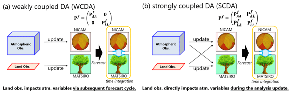
Figure 1Schematic images of (a) weakly coupled and (b) strongly coupled land–atmosphere data assimilation (DA) methods. Thin black arrows indicate model state updates through DA. Cyan double-headed arrows indicate land–atmosphere interactions between NICAM and MATSIRO during subsequent model forecasts. Here, panel (b) shows the fully strongly coupled DA method (cf. Fig. 2g). The image for NICAM was adapted from Satoh et al. (2014).
For the weakly coupled DA (hereafter WCDA) method, atmospheric observations are used only for updating NICAM state variables, and land observations are used for those of MATSIRO (Fig. 1a). That is, the cross-component error covariance between atmospheric and land variables is assumed to be 0 in WCDA (i.e., (Pf)AL=0 and (Pf)LA=0). Thus, impacts of atmospheric observations can propagate to land model states, and vice versa, only through interactions between NICAM and MATSIRO during model forecasts. For the strongly coupled DA (hereafter SCDA) method, the cross-component covariance is estimated based on ensemble forecasts (i.e., (Pf)AL≠0, (Pf)LA≠0, or both are nonzero matrices). Therefore, atmospheric or land observations are used to update both NICAM and MATSIRO variables based on the cross-component covariance (Fig. 1b). SCDA extracts more information than WCDA from the same observations if an appropriate forecast error covariance (Pf)αβ is applied.
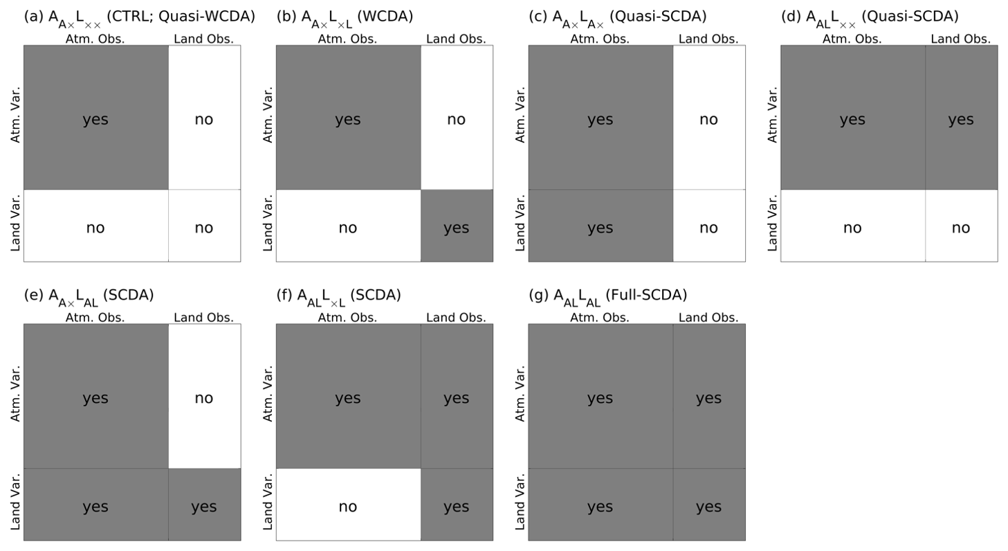
Figure 2Schematic plots of seven DA experiments for (a) (CTRL; quasi-WCDA), (b) (WCDA), (c) (quasi-SCDA), (d) (quasi-SCDA), (e) AA×LAL (SCDA), (f) AALL×L (SCDA), and (g) AALLAL (full-SCDA). The vertical axis represents atmospheric or land variables, and the horizontal axis shows observations. The shading of variables matches that of the observations used for their updates. White areas with “no” indicate error correlations that are assumed to be zero in DA. Gray areas with “yes” indicate error correlations that are included in DA.
This study considers seven coupled DA experiments (Fig. 2). Referring to Penny and Hamill (2017), we classify these experiments into five categories: quasi-WCDA, WCDA, quasi-SCDA, SCDA, and fully SCDA. Here we introduce identifiers (IDs) indicating which observation type is assimilated for each model. This study defines “A” and “L” as representations of the atmospheric and land, respectively. The IDs are defined as follows: “AA×” represents that assimilating only atmospheric observations to update the atmospheric model; “AAL” signifies that assimilating both atmospheric and land observations to update the atmospheric model; “LA×” denotes that assimilating only land observations to update the land model; “L×L” indicates that assimilating only land observations to update the land model; “LAL” corresponds to that assimilating both atmospheric and land observations to update the land model; and finally, “” represents that no observation is assimilated to update the land model.
For example, “” indicates that atmospheric observations are used to update the NICAM variables, while no observations are assimilated for the land model (Fig. 2a). This experiment is considered quasi-WCDA and is equivalent to the standard NICAM-LETKF system without SM DA or the control case (hereafter CTRL). “” stands for WCDA (Fig. 2b), while “AALLAL” signifies fully SCDA (hereafter full-SCDA; Fig. 2g). The remaining four experiments are treated as quasi-SCDA (Fig. 2c and d) and SCDA (Fig. 2e and f).
This study designs specific configurations of SCDA and WCDA to investigate whether updating MATSIRO variables through assimilating particular atmospheric observations has a beneficial impact. This investigation aims at finding the best-performing coupled land–atmosphere DA that consists of updates with a beneficial effect for the experimental setting of the present study. The best-performing approach might be different if we use different DA configurations or change the experimental settings, such as resolution and DA frequency.
2.3 Atmospheric data
The original NICAM-LETKF system assimilates conventional observations from the NCEP operational system (a.k.a. NCEP PREPBUFR), satellite radiance from Advanced Microwave Sounding Unit-A (AMSU-A), and the near-real-time version of Global Satellite Mapping of Precipitation (GSMaP_NRT). The dataset includes a number of different types of data: radiosondes, wind profilers, aircraft reports, surface pressure, atmospheric motion vectors, and surface winds derived from satellite observations. The channel selections for satellite radiances are 6, 7, and 8 for AMSU-A. The stratospheric sensitive channels are not assimilated in this study, considering the relatively low top level of the NICAM in this study (40 km). The satellite radiance scans and air mass biases are adaptively estimated and corrected at each data assimilation cycle. This experimental setting followed the operationally running NICAM-LETKF system. In this study, we use these data as atmospheric observations (cf. Table 1 of Kotsuki et al., 2019a). For further details of the assimilation methods used for these observations, we refer readers to previous studies (Terasaki et al., 2015; Kotsuki et al., 2017a; Terasaki and Miyoshi, 2017).
2.4 Soil moisture data
Satellite instruments can measure several land variables, including SM, surface skin temperature, and snow depth. Previous studies have found that land surface models tend to overestimate SM relative to SM data derived from satellite observations (Bindlish et al., 2018). GLDAS also shows larger SM values than satellite-based data (Bi et al., 2016). The significant bias between the model-based estimate and observation is unfavorable for DA. Prior to DA experiments, we compare spatial distributions of climatological SM for NICAM and satellite-based observations from the Soil Moisture and Ocean Salinity (SMOS; https://smos-diss.eo.esa.int/oads/access/, last access: 14 October 2023) and the Advanced Microwave Scanning Radiometer 2 of Global Change Observation Mission – Water (GCOMW/AMSR-2; https://lance.nsstc.nasa.gov/amsr2-science/, last access: 14 October 2023). We can see that NICAM SM is greatly biased compared to these satellite-based data (Fig. 3a, c, and d). In contrast, the bias of SM in NICAM relative to GLDAS is much smaller than that relative to SMOS and GCOMW/AMSR-2.
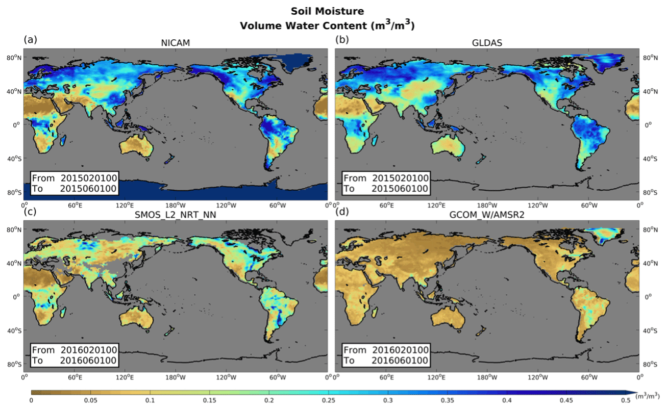
Figure 3Spatial patterns of soil moisture (m3 m−3) for NICAM, GLDAS, SMOS_L2_NRT_NN, and GCOM_W/AMSR2, averaged over February to June in 2015 (a, b) and 2016 (c, d).
Hoover and Langland (2017) assimilated pseudo-radiosonde observations from an independent atmospheric reanalysis system. They mentioned that assimilating reanalysis data from an advanced system significantly reduced biases in atmospheric temperature and geopotential height. As a first step, this study takes a similar approach and assimilates SM from GLDAS to avoid using satellite observation data which usually contain significant bias.
It is generally known that satellite, remote sensing, and model datasets have different mean SM values. Since we do not know the true mean values in remote sensing or model outputs, we cannot attribute these differences in these mean to bias in any specific data source. Satellite retrieval and model averages are determined by the parameters used in the retrieval and surface models, but we also do not know what those parameters should be. Therefore, the standard approach in SM data assimilation is to remove the difference between modeled and observed SM averages and then assimilate only the temporal anomalies in the observed SM values. Since it is crucial to have unbiased model and observation states to ensure the DA assumption is correct, several processes are proposed (Dee, 2005). For example, Reichle and Koster (2004) suggest a simple method to remove strong biases between satellite-based and model-based data, in which they match the cumulative distribution functions (CDFs) of the satellite and model data (a.k.a. CDF matching approach). On the other hand, several previous studies have successfully performed data assimilation without bias correction (e.g., De Lannoy et al., 2007; Bosilovich et al., 2007; Reichle et al., 2010; Honda et al., 2018). For example, Honda et al. (2018) demonstrated that assimilating geostationary satellite infrared radiance observations without bias correction every 10 min reduced the bias between the forecast and observations, leading to improved analysis without causing inconsistencies in the model states. Following the success of these previous studies, the present study assimilates SM data without bias correction. As shown later in Sect. 4a, the bias between the forecast and observation becomes negligible after a 1-month spin-up period when SM from GLDAS is assimilated every 6 h. Consequently, assimilating SM data without bias correction yields improvements in prediction accuracy of atmospheric variables. Since employing bias correction techniques and assimilating real satellite-sensed SM data could potentially lead to further enhancements, such endeavors are important subjects for future studies.
We perform QC using flags provided with the satellite observation data. In addition, as applied for PREPBUFR and GSMaP_NRT observations, we simply apply a gross error check for SM in which observations are rejected when the observation-minus-forecast value is greater than 10 times the observation error standard deviation (Terasaki et al., 2015).
GLDAS is a research-oriented land surface reanalysis system that produces spatiotemporally continuous global SM data. The GLDAS system integrates a suite of land surface models, which include the Noah, Community Land Model, Variable Infiltration Capacity, Mosaic, and Catchment. These land surface models provide physically based simulations of surface conditions, and each model has strengths and weaknesses depending on the applications. Among them, this study uses Noah-model-based SM data (GLDAS Noah Land Surface Model L4 Version 2.1; Chen et al., 1996; Koren et al., 1999). We only assimilate first-layer SM since satellite measurements cannot observe deep-layer SM. GLDAS provides 3-hourly SM at a spatial resolution of 0.25∘ × 0.25∘. As these data are denser than those of NICAM (112 km and 6-hourly resolution), we reduce the data density spatially and temporally. The original SM data are averaged within a NICAM model grid so that each observation corresponds to one model grid point. The original 3-hourly data are also averaged over 6 h. These spatial and temporal data aggregation processes are carried out simultaneously prior to data assimilation.
The GLDAS Version 2.1 simulation is forced with National Oceanic and Atmospheric Administration (NOAA)/Global Data Assimilation System (GDAS) atmospheric analysis fields (Derber et al., 1991), the disaggregated Global Precipitation Climatology Project (GPCP) V1.3 Daily Analysis precipitation fields, and the Air Force Weather Agency's AGRicultural METeorological modeling system (AGRMET) radiation fields. Because GLDAS uses observed precipitation of GPCP, SM in GLDAS is considered better than that of MATSIRO, which uses precipitation forecasts from NICAM to drive the land surface model. Since SM in NICAM has a large bias against the satellite-based product (Fig. 3), this study assimilates SM from GLDAS as pseudo-observations as Hoover and Langland (2017) and verifies forecasted SM compared to GLDAS.
This study performs 40-member NICAM-LETKF experiments. NICAM ensemble forecasts are performed for 9 h intervals, and observation data from the last 6 h period are assimilated. The initial ensemble members of the experiments are obtained from the 1st–40th members of a long-term 128-member NICAM-LETKF experiment (Terasaki et al., 2019). This means the initial ensemble spread of SM relies on initial conditions perturbed by the ensemble NICAM forecasts. Covariance localization in LETKF is applied to the observation error covariance R so that distant observations have smaller impacts on the analysis (Hunt et al., 2007; Miyoshi and Yamane, 2007). Gaussian functions are used for horizontal and vertical localization, given by
where f is the localization function, and dh and dv are the horizontal distance (km) and vertical difference (log (Ps)) between the analysis model grid point and the observation, respectively. Standard deviations (SDs) of σh and σv are 400 km and 0.4 natural log pressure, as implemented by Terasaki et al. (2019). The localization function is replaced by zero beyond . Land (atmospheric) observations are assimilated into the atmospheric (land) model using the same vertical localization scale. For land observations, surface pressure (Ps) is assigned for the observed height. This study uses relaxation to prior spread (RTPS; Whitaker and Hamill, 2012) for covariance inflation. For atmospheric variables, the relaxation parameter is set to 0.90, which is determined through sensitivity tests (Kotsuki et al., 2017b). As mentioned in Sect. 2.2, the original NICAM-LETKF method, which assimilates only atmospheric observations, is referred to as the control experiment. These experimental settings have been widely applied in previous NICAM-LETKF experiments (e.g., Kotsuki et al., 2018, 2019a). In addition to atmospheric observations, this study assimilates SM data as hydrological land observations. The observation error SD of SM is estimated at 0.05 (m3 m−3) based on the innovation statistics of Desroziers et al. (2005) (cf. Appendix A). We perform one control experiment and six SM DA experiments, as shown in the schematic images of Fig. 2.
Maintaining the ensemble spread is important in the EnKF. We initially expected that ensemble forecasts could sufficiently maintain the ensemble spreads of MATSIRO variables due to physical coupling with NICAM. However, the ensemble spread of SM in MATSIRO decreased rapidly after initiating assimilation of SM from GLDAS in our preliminary experiment (not shown). We were unable to mitigate this rapid reduction of ensemble spreads even by applying RTPS with relaxation parameter α=0.90. This outcome seems to be related to two fundamental challenges: (1) the land models are typically more dependent on external forcing, rather than being modeled as a chaotic dynamical system dependent on initial conditions, and (2) the timescales for dynamical changes in land models are much longer than those in atmospheric models. The latter implies that the land model is likely to have a long memory beyond 6 h for SM. In the case of assimilating SM with atmosphere–land coupled models, SM observations correspond to the slow mode, and atmospheric variables correspond to the fast mode. Therefore, offline land DA systems usually inflate the ensemble spread by adding random noise to atmospheric forcing or observational data. For example, Reichle et al. (2002) added perturbations to the ensemble forecasting system, specifically to forcing and to the model states variables, to account for sources of model error in the land model forecast to generate an ensemble representative of the model forecast uncertainty. In the current study, we use RTPS to maintain the ensemble spread of SM in MATSIRO to avoid the ensemble becoming too confident. In addition, land DA experiments with the land–atmosphere system would represent model errors to some extent since each land model is driven by different forcing. The relaxation parameter for SM is set to α=1.00 so that the analysis ensemble spread is equivalent to the forecast ensemble spread. For further details on creating ensemble spreads for land models, we encourage readers to review the summary presented in Draper (2021).
Further, since satellite-borne microwave sensors can measure only surface layer SM, we explore better DA strategies that will be applicable to satellite observations. Thus, we only use SM data in the surface layer (0–0.1 m) provided by GLDAS. In our experiments, GLDAS SM data are assimilated into the topmost layer of MATSIRO (0–0.05 m). Although analyzing deeper layers of SM is essential to take advantage of land–atmosphere coupling, this study focuses on the surface layer where feedbacks to the atmosphere would be more pronounced than in deeper layers. Note that the present experimental setting for assimilating GLDAS SM data may result in more significant impacts than the experiments with actual satellite observation intervals.
We first perform a spin-up NICAM-LETKF experiment from June to September 2014 by assimilating only atmospheric observations. The initial NICAM ensemble conditions are taken from the long-term NICAM-LETKF experiment of Terasaki et al. (2019). DA experiments are performed for 13 months, from 00:00 UTC 1 October 2014 to 18:00 UTC 30 November 2015. The first month (October 2014) is considered a spin-up period, and the results for the latter 12 months are used for validation.
In Sect. 4.1, the data are used for validation to check if the assimilation behaves as expected (i.e., the analysis departures of SM are reduced by the assimilation). In addition, we also use SM from ERA5 reanalysis data (Hersbach et al., 2020) as an independent dataset for validation scores. We evaluate atmospheric variables against the ERA5 reanalysis data in Sect. 4.2. The analysis of land variables is performed separately from the atmospheric analysis in the ERA5 by assimilating screen-level temperature, dewpoint, and synoptic observations with the optimal interpolation. While ERA5 assimilates no SM observation, it assimilates many more satellite observations than the NICAM-LETKF, such as from the Microwave Humidity Sounder and Advanced Technology Microwave Sounder. Therefore, validating NICAM-LETKF atmospheric fields relative to the ERA5 is reasonable. Furthermore, as described, SM of GLDAS can be considered better than the NICAM-LETKF because it is derived by observed precipitation. Hence, in the following sections, we demonstrate that the assimilation of SM from GLDAS has a beneficial effect on atmospheric fields in NICAM-LETKF, as verified by comparison with ERA5.
4.1 Impacts on soil moisture
We first examine the impacts of SM assimilation on MATSIRO. Figure 4 compares the global bias patterns for the prior state of SM at the near-surface layer (i.e., 0–0.05 m) relative to GLDAS, averaged over a 12-month period from November 2014 to October 2015. Three panels show the results for (CTRL; quasi-WCDA), (WCDA), and AALLAL (full-SCDA). (CTRL) shows dry biases relative to GLDAS in general, especially in the continents of Africa, South America, Australia, and central Eurasia (Fig. 4a). Assimilating SM into MATSIRO successfully mitigates these SM biases (Fig. 4b and c). Furthermore, assimilating SM mitigates the wet SM bias in regions where SM is overestimated in (CTRL). Therefore, the newly developed coupled land–atmospheric DA system successfully assimilates SM data into MATSIRO, and we confirm the developed DA system works well. These results are expected and not surprising because forecasts are validated using the same data as observations. No notable differences are observed in global bias patterns between (WCDA) and AALLAL (full-SCDA) in global bias patterns (Fig. 4b and c).
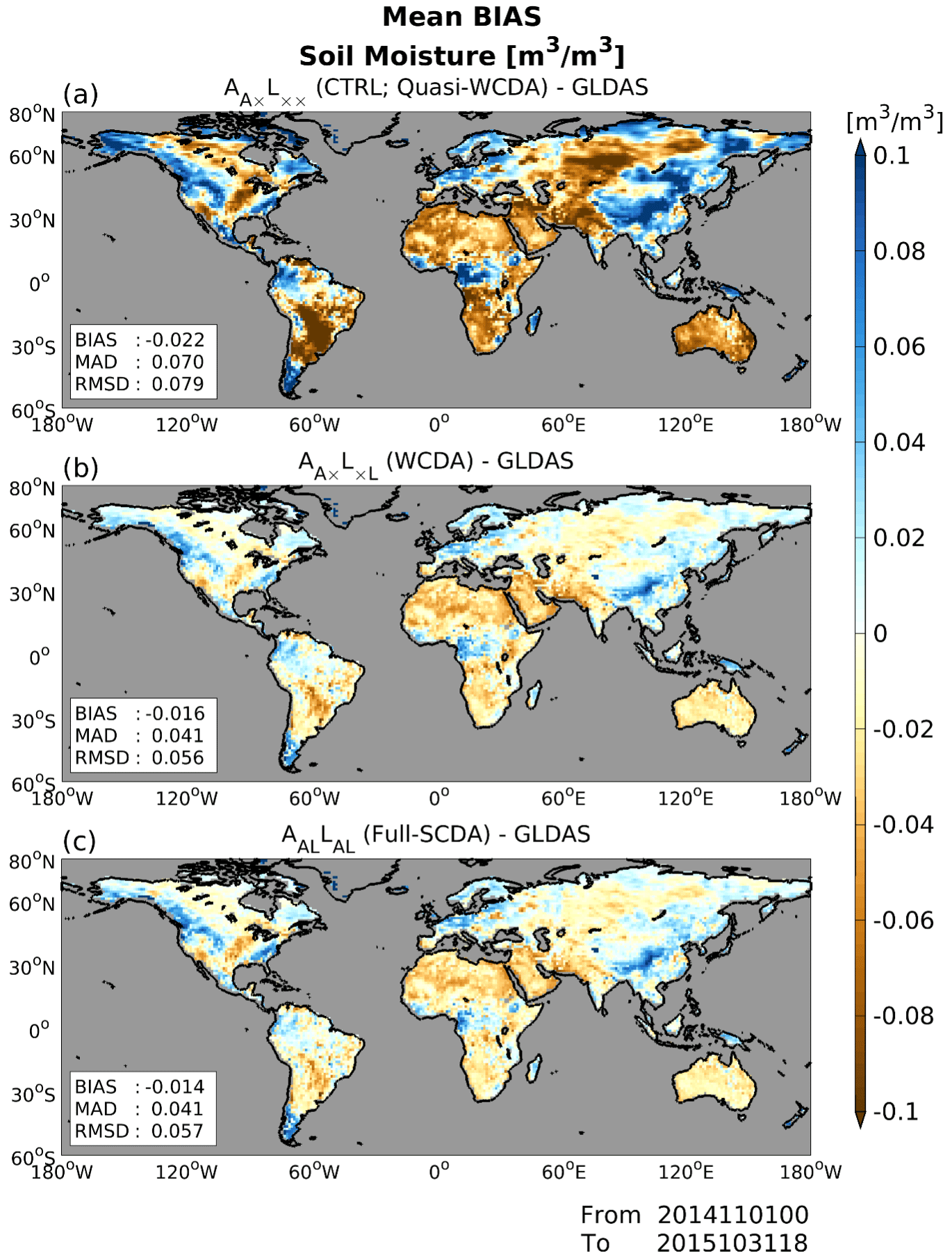
Figure 4Global patterns of 6 h forecast bias for soil moisture (SM; m3 m−3) relative to GLDAS for (a) (CTRL; quasi-WCDA), (b) (WCDA), and (c) AALLAL (full-SCDA), averaged over 12 months from November 2014 to October 2015. The blue and brown colors represent overestimated and underestimated SM values relative to GLDAS, respectively.
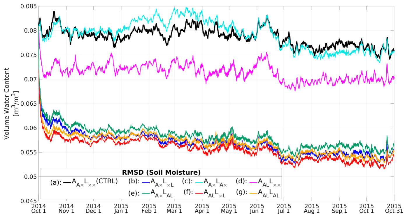
Figure 5Time series of global-mean forecast root mean square differences (RMSDs) for soil moisture (SM; m3 m−3) relative to GLDAS. The black, blue, cyan, magenta, green, red, and yellow lines indicate (a) (CTRL; quasi-WCDA), (b) (WCDA), (c) (quasi-SCDA), (d) (quasi-SCDA), (e) AA×LAL (SCDA), (f) AALL×L (SCDA), and (g) AALLAL (full-SCDA) experiments, respectively. Experiments (a)–(g) correspond to the DA patterns (a)–(g) shown in Fig. 2.
Figure 5 shows the time series of global-mean root mean square differences (RMSDs) for SM relative to GLDAS. All experiments that assimilate SM have smaller errors in SM than those in (CTRL; Fig. 5a). Although (WCDA; Fig. 5b) and AALLAL (full-SCDA; Fig. 5g) show reduced errors, no clear difference is apparent between the two experiments. Among the seven experiments, AALL×L (SCDA; Fig. 5f) results in the smallest SM error. In this experiment, SM observations are used for updating both NICAM and MATSIRO, whereas atmospheric observations are used only for updating NICAM and not for MATSIRO. Since AALL×L (SCDA) results in better SM estimation than AALLAL (full-SCDA; Fig. 5g), we can see that updating SM in MATSIRO through assimilation of atmospheric observations has a detrimental impact on SM in the experimental settings of this study.
Such detrimental impacts are also found by comparing other cases, such as (WCDA; Fig. 5b) and AA×LAL (SCDA; Fig. 5e). The larger error in AA×LAL (SCDA) than in (WCDA) arises from inaccurate covariance estimates between atmospheric observations and land variables due to insufficient ensemble size. Ensemble-based DA can provide spurious error correlations when the ensemble size is small. Assimilating observations based on spurious error covariances generally degrades the analysis results (cf. variable localization of Kang et al., 2011). Moreover, the difference in timescale between the atmospheric and terrestrial models may have a dominant influence, which could be verified by experiments using a short assimilation window. Such further investigation of the assimilation window is essential for future studies of land–atmosphere coupled DA.
(quasi-SCDA; Fig. 5c) shows similar RMSDs to those of (CTRL; quasi-WCDA), which implies that atmospheric observations have neither beneficial nor detrimental impacts on updating SM. Because many types of atmospheric observations are assimilated in this study, clarifying impacts of individual observation type is complicated. The results might be changed if we assimilate only one kind of atmospheric observation, such as precipitation data, with the variable localization. Accurate estimation of (Pf)AL by increasing the number of ensembles might reduce the RMSD of (quasi-SCDA). Penny et al. (2019) also faced this kind of problem when assimilating slower ocean observation data into an atmosphere–ocean model with coupled DA. Penny et al. (2019) found that it was more difficult to use slow-mode observations (from the ocean) to update the fast-mode observations (atmosphere). They overcame this problem by using larger ensembles and increasing the analysis update and observation frequency. As discussed for maintaining ensemble spreads for SM, SM observations correspond to the slow mode, and atmospheric variables correspond to the fast mode in our experimental settings. Therefore, applying the approach by Penny et al. (2019) may further improve SCDA.
We can say that Fig. 5 represents the error correlation between the SM observations and the atmospheric model variables, showing that it is more reliable than the correlation between the atmospheric observations and the SM variable from the land model. In terms of reducing the errors in SM, the optimal coupled DA method in our experimental setting is AALL×L (SCDA). The errors in SM can be reduced by updating atmospheric and land variables through the assimilation of SM. Several previous studies have found that it is important to correct the “upstream” dynamics in the coupled system (e.g., by Sluka et al., 2016). In other words, since the atmosphere strongly drives the land via surface forcing, correcting the atmospheric variables would improve forecasts of the coupled land surface model. From the point of view of the land model, the SM can be updated accurately by assimilating the observed SM directly. Attempting to use fast-varying atmospheric observations for updating SM would lead to suboptimal analysis because of the non-perfect ensemble-based error covariance estimate between atmospheric observations and modeled SM. In contrast, the detrimental impacts of updating atmospheric variables by (Pf)AL cancel out the beneficial impacts of updating SM by (Pf)LA. Therefore, for our model configuration and DA design, AALLAL (full-SCDA) is less effective than AALL×L (SCDA). This problem might occur because the DA approach degrades the analysis when assimilating atmospheric data into the land model. The approaches for atmosphere–ocean coupled DA suggested by Penny et al. (2019) could solve the problem, which will be an important future subject to improve SCDA even more.
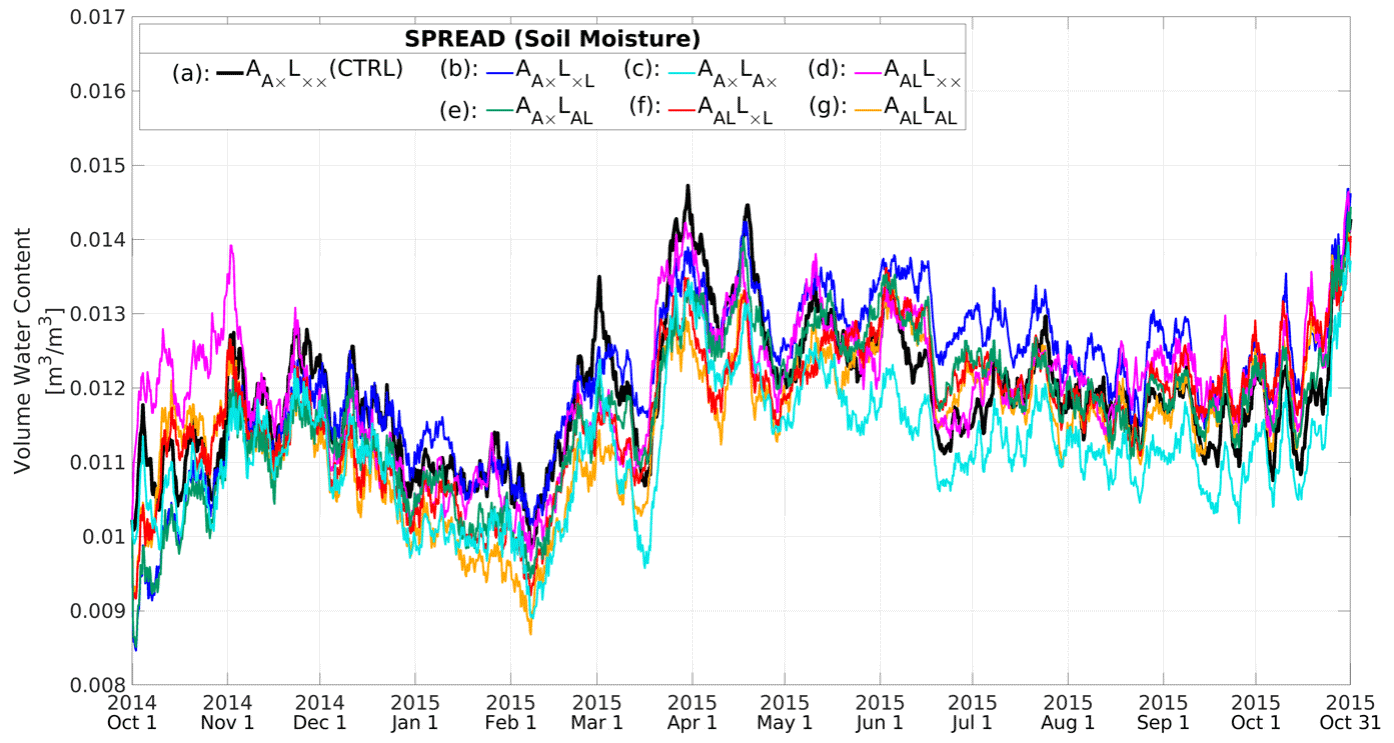
Figure 6 shows the time series of ensemble spread of SM. Since RTPS is used with a relaxation parameter of 1.0 for land variables, the ensemble spread does not change during DA. Because no significant difference is observed in the ensemble spreads among experiments, the difference in RMSDs relative to GLDAS must originate from the difference in the update strategy. The ensemble spread of (quasi-SCDA; Fig. 6c) is the smallest among these cases, which means the atmospheric observations have collapsed the spread more than any other configurations. By assimilating the atmospheric observations into the land model, the impact of the land observations becomes less, leading to the detrimental effect observed in those cases. This could also be related to the balance between the errors on the atmospheric observations and the spread of the land model variables. This indicates that the atmospheric observation error should be inflated when applied to the land DA via SCDA. The process filters out the impact of high variability in the atmosphere, similar to adding errors of representativeness in the spatial dimension.
Figure 7 shows the global patterns of differences in analysis RMSDs for SM, averaged over a 12-month period from November 2014 to October 2015. Here, we discuss three experiments: (WCDA), AALLAL (full-SCDA), and AALL×L (SCDA), which are the best three experiments in terms of errors in SM, as shown in Fig. 5. First, we compare (WCDA) and AALL×L (SCDA). Figure 7a suggests that updating atmospheric variables with SM DA generally has beneficial impacts on SM. In South America, the Arabian Peninsula, and India, beneficial impacts are seen in regions where (CTRL) shows a dry bias in SM in Fig. 4. Additionally, beneficial impacts are apparent in central Africa, where (CTRL) has a wet bias in SM. In contrast, SM DA has moderate impacts in North America and Eurasia. In these areas, AALLAL (full-SCDA) performs worse than (WCDA; Fig. 7b), suggesting that assimilating atmospheric observations to update SM in MATSIRO would be detrimental in the experimental settings of this study. Therefore, eliminating the updates of MATSIRO with atmospheric observations has beneficial impacts for SCDA (Fig. 7c).
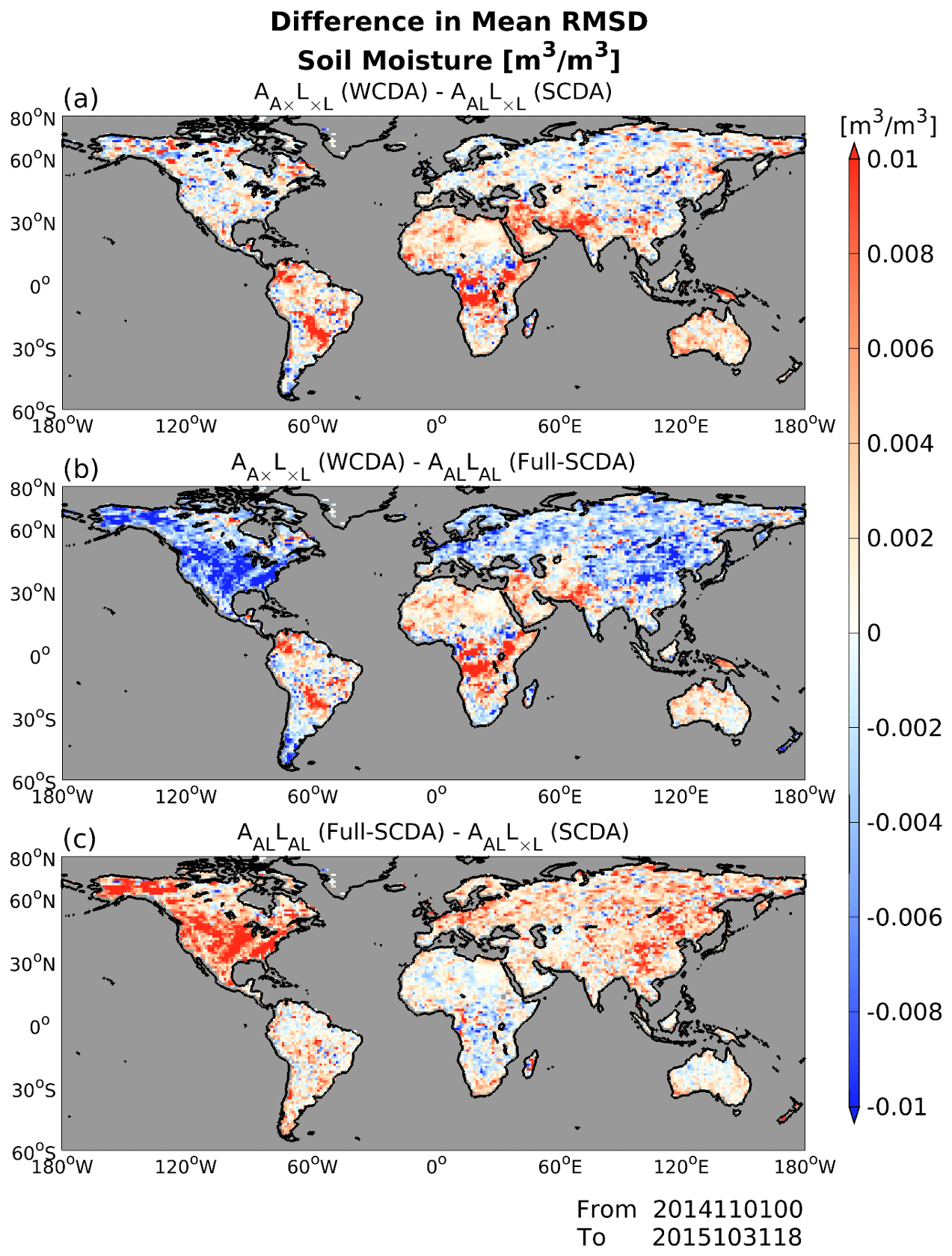
Figure 7Global patterns of soil moisture analysis RMSD (m3 m−3) relative to GLDAS averaged over 12 months from November 2014 to October 2015: (a) difference between (WCDA) and AALL×L (SCDA), (b) difference between (WCDA) and AALLAL (full-SCDA), and (c) difference between AALLAL (full-SCDA) and AALL×L (SCDA). Warm colors indicate that the latter experiments providing smaller scores than the former experiments, whereas cool colors indicate larger scores of the latter methods.
We also investigate the SM correlations between GLDAS and the results of the experiments (Fig. 8). We can see that the correlation to GLDAS is larger in the regions where positive impacts are observed in Fig. 7. Figure 9 shows the results of the two-sample t test. Time series of absolute bias of SM analysis relative to GLDAS are sampled from November 2014 to October 2015. When the p values at a point are smaller than 5 %, the null hypothesis at the 95 % confidence level is rejected, implying a significant difference. By the significance test, we can see the significant differences between the experiments over broad regions. The significant differences between methods (WCDA) and AALL×L (SCDA) are mainly located in the areas where the bias was relatively substantial in Fig. 4a (Fig. 9a). From Figs. 8 and 9, we can reconfirm the points described in the comments about Fig. 7: (1) using SM to update atmospheric variables has positive effects, especially in areas where there are dry biases; (2) areas where there are wet biases are mitigated by SM DA; and (3) updating SM with atmospheric observations has detrimental effects, leading to the results of AALLAL (full-SCDA) experiments.
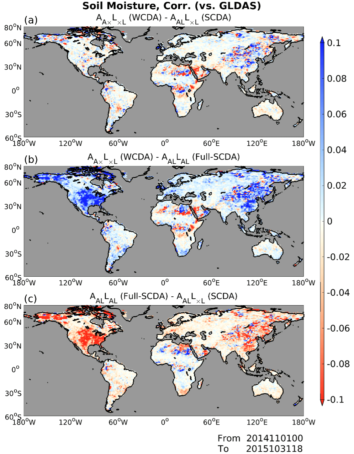
Figure 8Global patterns of soil moisture analysis correlation relative to GLDAS sampled over 12 months from November 2014 to October 2015: (a) difference between (WCDA) and AALL×L (SCDA), (b) difference between (WCDA) and AALLAL (full-SCDA), and (c) difference between AALLAL (full-SCDA) and AALL×L (SCDA). Warm colors indicate that the latter experiments providing smaller scores than the former experiments, whereas cool colors indicate larger scores of the latter methods.
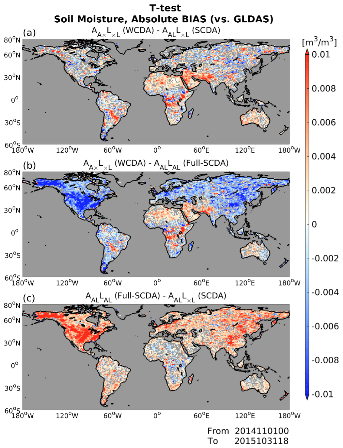
Figure 9Global patterns of soil moisture analysis absolute bias (m3 m−3) relative to GLDAS: (a) difference between (WCDA) and AALL×L (SCDA), (b) difference between (WCDA) and AALLAL (full-SCDA), and (c) difference between AALLAL (full-SCDA) and AALL×L (SCDA). Only the areas where the t test gives significant differences (the p value < 5 %) are colored, sampling with time series of soil moisture analysis from November 2014 to October 2015. Areas without significant differences are grayed out.
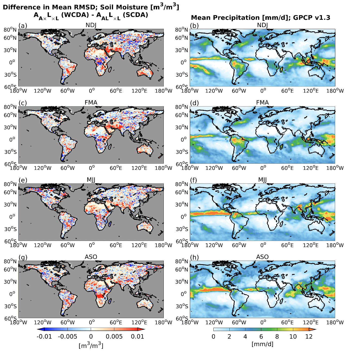
Figure 10Global patterns of soil moisture analysis RMSD (m3 m−3) relative to GLDAS (a, c, e, g) and spatial patterns of observed precipitation of GPCP version 1.3 (mm d−1; b, d, f, h). Results are averaged over 3 months: (a, b) November 2014 to January 2015, (c, d) February to April 2015, (e, f) May to July 2015, and (g, h) August to October 2015. Panels (a), (c), (e), and (g) show the difference between (WCDA) and AALL×L (SCDA). In panels (a), (c), (e), and (g), warm colors indicate that AALL×L (SCDA) is performing better than (WCDA), whereas cool colors indicate a worse performance of AALL×L (SCDA).
We also investigate the seasonal differences in the relationship between precipitation and SM. Figure 10 compares the difference of SM analysis RMSD relative to GLDAS between (WCDA) and AALL×L (SCDA; Fig. 10a, c, e, and g), with observed precipitation of GPCP version 1.3 (Fig. 10b, d, f, and h). The SCDA experiment shows improvements in the Sahel and equatorial Africa from May to October (Fig. 10e and g) compared to the period from November to April (Fig. 10a and c). These regions are known to be “hotspots” where SM affects precipitation during June–August (Koster et al., 2004). SM assimilation by SCDA would benefit from updating atmospheric variables in the hotspot regions. On the other hand, the distribution of precipitation from November to April tends to shift slightly southwards, resulting in decreased precipitation in previously defined hotspots (Fig. 10b and d). Therefore, the advantages of updating atmospheric variables using SM data are not as evident in these areas in our experiments (Fig. 10a and c). This period includes the summer season in the Southern Hemisphere. For instance, we can confirm a notable increase in precipitation in South America (Fig. 10b and d). Correspondingly, the advantages of using SCDA in that area become more pronounced. The Arabian Peninsula is another region where the advantages of SCDA stand out during this season, despite being an area with scarce rainfall throughout the year and minimal seasonal differences. Therefore, comparison of results from November to April (Fig. 10a–d) with those from May to October (Fig. 10e–h) implies that the locations of the “hotspots” may vary depending on the season.
From the above results, it is clear that precipitation and SM are closely related. Given the seasonal variation in precipitation distribution, the regions that would benefit from updating atmospheric variables using SM data shift accordingly.
We also use ERA5 SM as an independent dataset for the validation scores, although so far, we have been using GLDAS to verify that the experimental setup works as expected. Figure 11 compares the global patterns of 6 h forecast bias in SM at near-surface layer as in Fig. 4 but relative to ERA5. We can see that (CTRL) shows large dry biases relative to ERA5 in South America and central Eurasia (Fig. 11a). The dry biases appear mitigated by updating MATSIRO with the SM of GLDAS. Furthermore, NICAM has a large dry bias in the center of the African continent relative to ERA5, which is not the case when compared to GLDAS in Fig. 4. There is a wet bias at the southern and northern ends of the African continent, which increases with the assimilation of SM, but the global-averaged scores show improvements compared to (CTRL; Fig. 11b and c). No notable differences are observed between (WCDA) and AALLAL (full-SCDA) in global bias patterns (Fig. 11b and c).
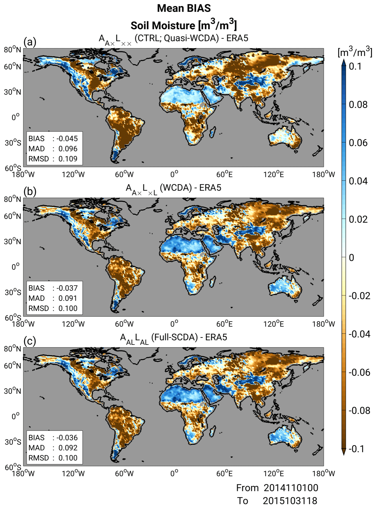
Figure 11Similar to Fig. 4 but showing 6 h forecast bias for soil moisture relative to ERA5 (m3 m−3).
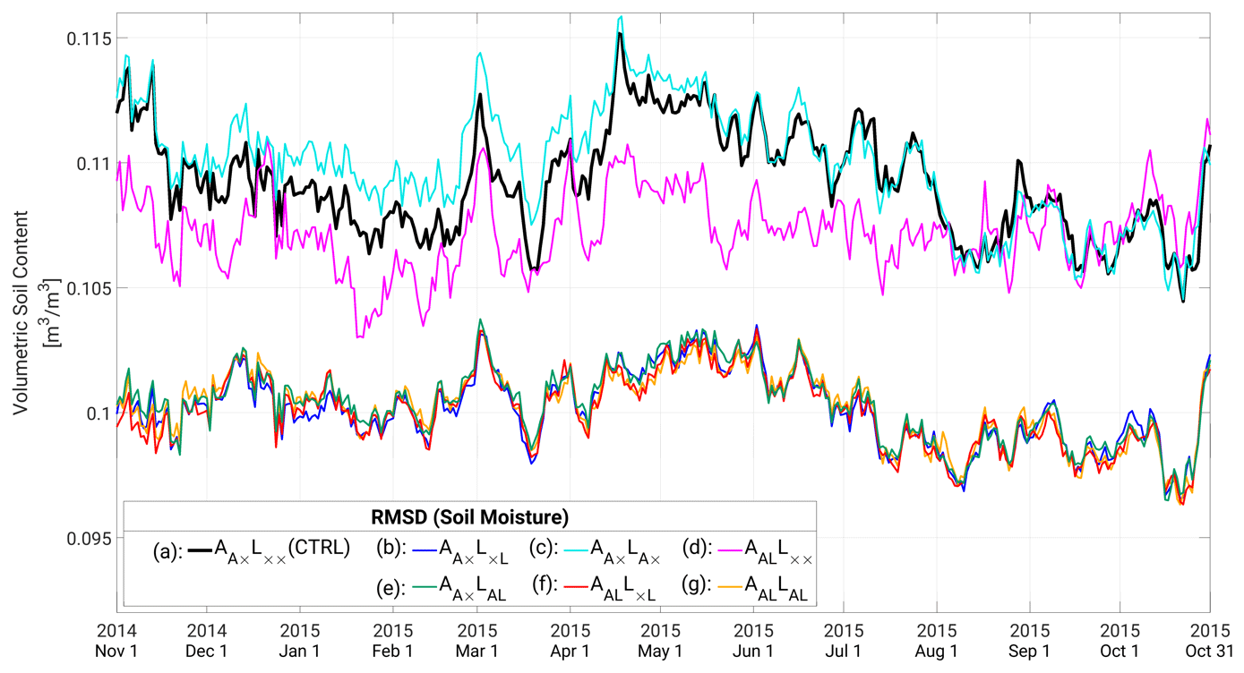
Figure 12 shows the time series of global-mean RMSDs for SM as in Fig. 5 but relative to ERA5. Similar to the results in Fig. 5, we can find the following features: all experiments that assimilate SM have smaller errors in SM than in (CTRL). (quasi-SCDA; Fig. 12c) shows larger RMSDs compared to those of (CTRL), whereas (quasi-SCDA; Fig. 12d) shows smaller RMSDs than (CTRL). This validation against ERA5 SM also supports the previously identified findings: updating atmospheric variables by SM DA is beneficial to improving SM forecasts, whereas updating the SM variable by assimilation of atmospheric observations results in detrimental impacts. The differences between the other four experiments, in which SM observations update the MATSIRO variables, are unclear, but they show a significant decrease in RMSDs compared to (CTRL).
Lastly, Fig. 13 compares the differences in analysis RMSD of SM relative to ERA5. We can see a meaningful benefit of having atmospheric model variables updated by SM observations where there was a robust dry bias, e.g., in the South American continent (Fig. 13a and b). On the other hand, there was originally a wet bias against ERA5, i.e., the Arabian Peninsula and north of the African continent, resulting in a modification effect. Furthermore, a feature not seen in Fig. 7 is that with ERA5 as reference data, there is no significant worsening of the MATSIRO variables by updating them with atmospheric observations (Fig. 13c).
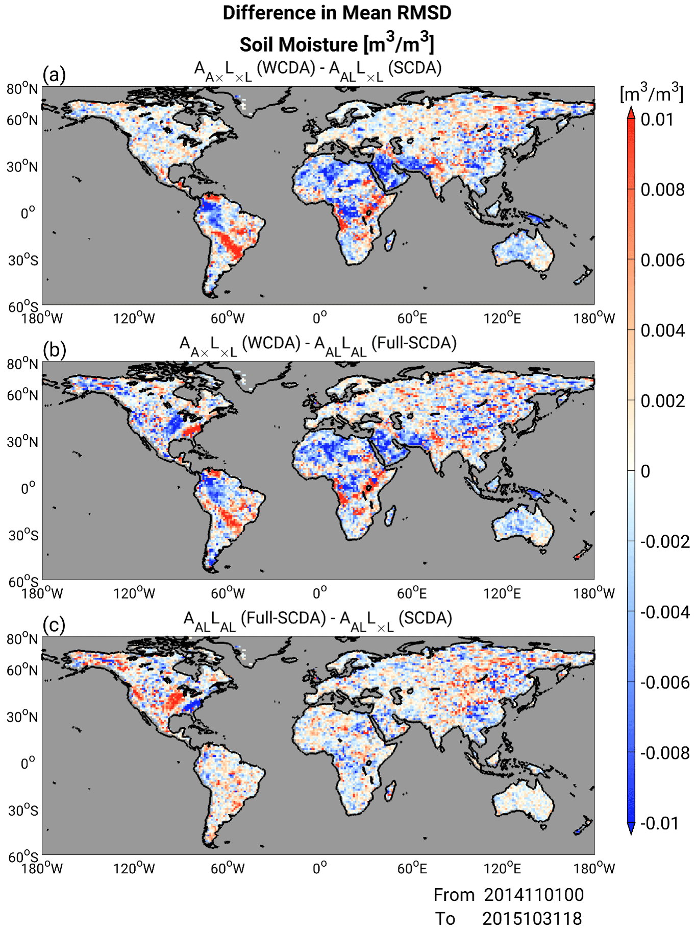
Figure 13Similar to Fig. 7 but showing global patterns of soil moisture analysis RMSD relative to ERA5 (m3 m−3).
The validation results using an independent dataset suggest that the experiments conducted in this study are functioning reasonably well. These findings support the notion that our experiments, which assimilate SM data from GLDAS without bias correction, can perform satisfactorily without violating the underlying assumptions of data assimilation. In this section, the results show that the assimilation of atmospheric observations can lead to detrimental effects on soil moisture analysis. It is crucial to note that this issue stems from the experimental setup rather than statistical aspects. The primary cause of these adverse effects would be the weak dynamical relationship between the lower troposphere and SM. We will explore the issues related to this physical relationship in the subsequent section.
4.2 Impacts on atmospheric field
Here, we investigate the impacts of assimilation of SM on atmospheric variables. Figure 14 shows the global patterns of forecast biases for temperature (K) in the lower troposphere (850 hPa) relative to the ERA5 reanalysis data averaged over 12 months from November 2014 to October 2015. Hereafter, we discuss the results of (CTRL) and three coupled DA experiments: (WCDA), AALL×L (SCDA), and AALLAL (full-SCDA). Figure 14a shows that (CTRL) has a warm temperature bias in regions with dry SM biases, as illustrated in Fig. 4 (e.g., South America, Africa, and Australia). In these regions, increasing SM values after assimilation of SM decreases temperature estimates in the lower troposphere (Fig. 14b–d), since more of the incoming solar and longwave radiation is converted to latent heat flux and less to sensible heat flux with greater SM. Compared to (WCDA), however, AALL×L (SCDA) and AALLAL (full-SCDA) show an overcooling effect for temperature in the continents of Africa and Australia (Fig. 14c and d). This overcooling effect is caused by the assimilation of SM into atmospheric variables in NICAM. The condition and type of soil determine the allocation of energy to latent and sensible heat flux. In areas with sufficient SM, evaporation is limited by the amount of available water, even though more evaporation is energetically possible. In such a case, the ratio of latent heat to sensible heat (i.e., Bowen ratio) will be determined by the surface temperature. In contrast, in a dry area, the ratio becomes smaller. In addition, the energy balance is led by the turbulent fluxes of sensible, latent heat, and the ground heat flux. The energy transfer from the surface to the atmosphere creates spatial pressure gradients that drive atmospheric circulation at various scales. Due to the factors above, the most appropriate setting was (WCDA) in our experiments. There are no remarkable changes in temperature over the ocean among the DA methods.
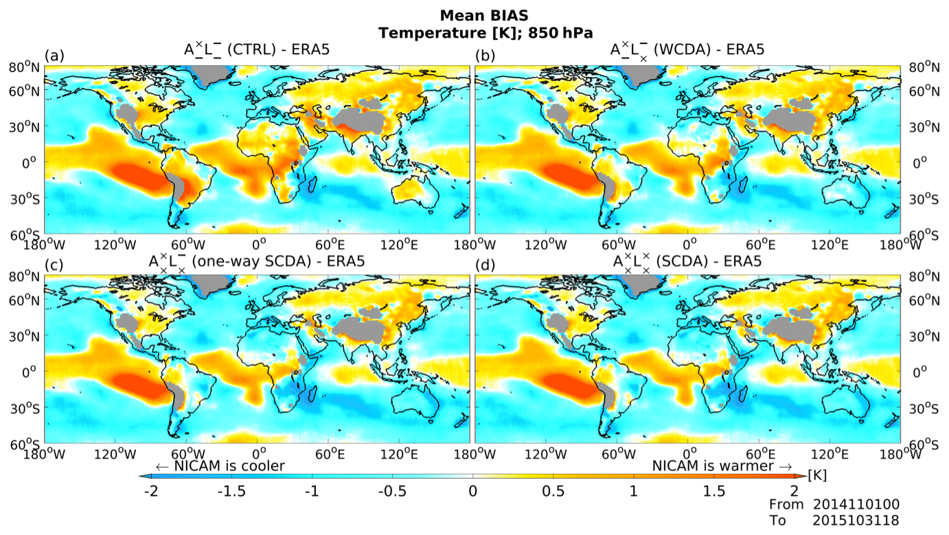
Figure 14Global patterns of forecast bias for temperature (K) at 850 hPa relative to ERA5 reanalysis values for (a) (CTRL), (b) (WCDA), (c) AALL×L (SCDA), and (d) AALLAL (full-SCDA), averaged over 12 months from November 2014 to October 2015. Red and blue colors represent warm and cold biases, respectively.
Table 1Averaged scores for bias, mean absolute difference (MAD), and RMSD for temperature at 850 hPa in Fig. 14. The biases and errors in (a) and (b) are averaged only over the ocean and only over land, respectively. The smallest errors are indicated by the bold font.
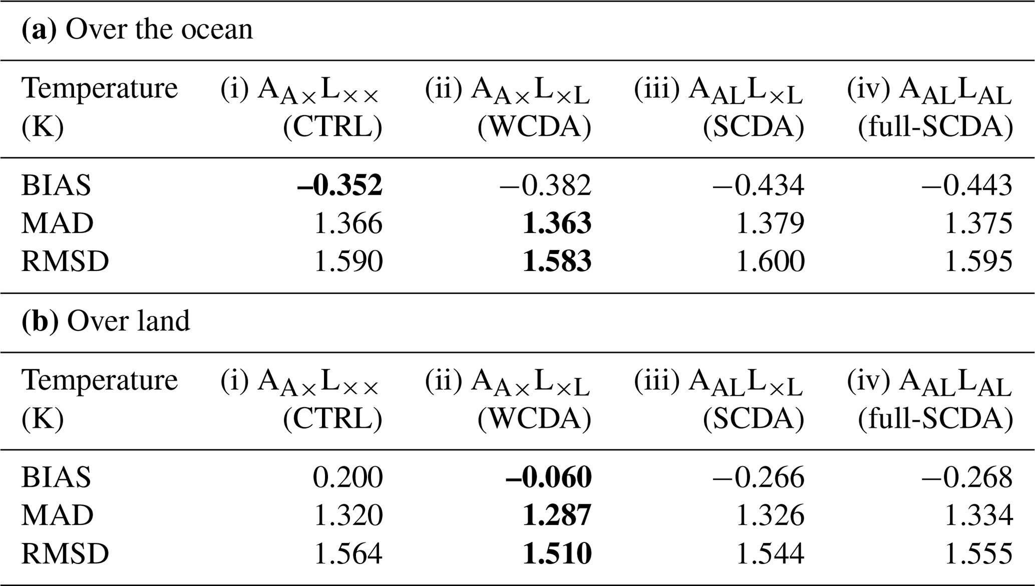
Table 1 summarizes the global-mean scores for bias, RMSD, and mean absolute difference (MAD) in temperature. Table 1a and b show these values averaged over the ocean and land, respectively. The errors in Table 1a differ less strongly than those in Table 1b, showing that assimilation of SM changes the temperature field mainly over land. The bias values in Table 1b show that (CTRL) has a warm temperature bias over land in general. Assimilating SM leads to a cooling effect, thereby mitigating the warm temperature bias. However, AALL×L (SCDA) and AALLAL (full-SCDA) decrease temperature too much, resulting in a cold bias. Consequently, (WCDA) results in the best temperature field among the four experiments in terms of temperature bias at 850 hPa. Assimilating SM with (WCDA) decreases the average temperature bias by 0.26 K over land. These changes over land do not propagate significantly to the temperature bias over the ocean.
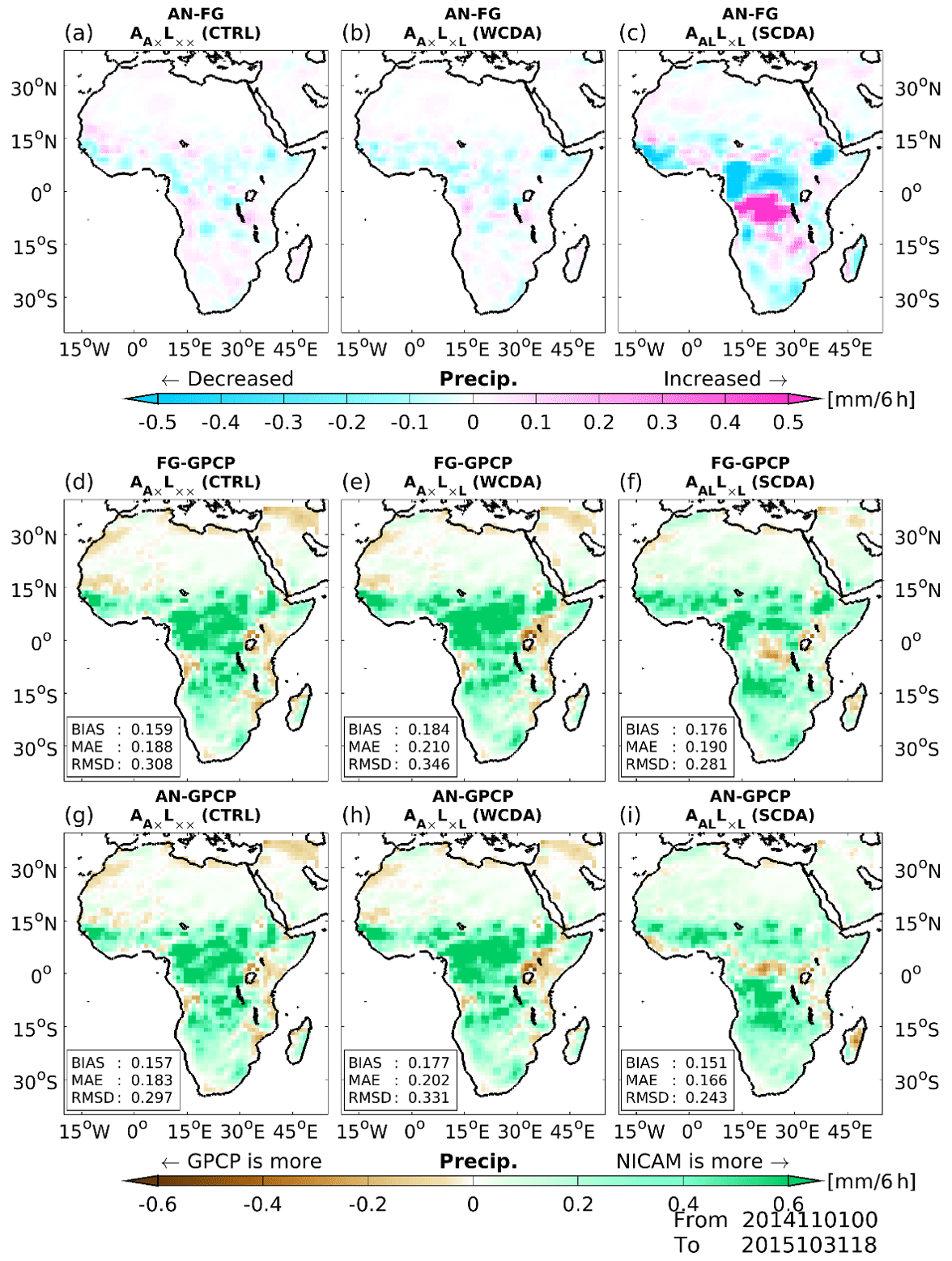
Figure 15Spatial patterns of analysis increments for precipitation (mm 6 h−1; a–c) and precipitation forecast biases (d–f) and analysis biases (g–i) relative to GPCP version 1.3 (mm 6 h−1), averaged over 12 months from November 2014 to October 2015. Magenta and cyan colors in panels (a)–(c) represent increased and decreased precipitation with DA, respectively. The green and brown colors in panels (d)–(i) represent overestimated and underestimated precipitation values, respectively, relative to GPCP. Panels (a), (d), and (g); (b), (e), and (h); and (c), (f), and (i) show the (CTRL), (WCDA), and AALL×L (SCDA) experiments, respectively.
We also investigate changes in the precipitation field, focusing on the continent of Africa, where large changes in SM occur due to SM DA (Fig. 4). Figure 15a–c show the spatial patterns of analysis increments for precipitation amount, averaged over 12 months from November 2014 to October 2015. Note that DA can be used for analyzing not only model diagnosed variables (i.e., model state variables) but also other outputs from the model. For example, Kotsuki et al. (2017a) analyzed precipitation using NICAM-LETKF, where precipitation is not part of the initial condition. Here, we compare analysis increments of model-like precipitation (cf. Fig. 3 of Kotsuki et al., 2017a). Since precipitation is classified as an atmospheric diagnosed variable, we observe increments in precipitation during the assimilation of atmospheric observations. The difference in precipitation analysis increments between (CTRL) and (WCDA) is insignificant (Fig. 15a and b). In contrast, precipitation in AALL×L (SCDA) can be affected by the assimilation of atmospheric and SM observations (Fig. 15c). In central Africa, where precipitation amount changes significantly with SM DA, the analysis increments shift noticeably. We observe negative analysis increments where SM in (CTRL) is drier and positive increments when it is wetter. This suggests that coupled land–atmospheric DA performs reasonably, as assimilating SM data increases (decreases) precipitation in areas where NICAM has a dry (wet) bias (Fig. 4a).
Spatial patterns of forecast and analysis biases in precipitation relative to GPCP version 1.3 estimates are shown in Fig. 15d–i. GPCP, which provides global precipitation data through the merging of various satellite and gauge datasets, is considered to include the best global precipitation estimates in the climate research community (Kotsuki et al., 2019c). First-guess precipitation in (CTRL) has a positive bias relative to GPCP (Fig. 15d; +0.159 mm 6 h−1), and this overestimation is intensified in (WCDA; +0.184 mm 6 h−1). In contrast, the first-guess precipitation bias in AALL×L (SCDA; +0.176 mm 6 h−1) is smaller than that in (WCDA), although both experiments assimilate SM (Fig. 15e and f). In (CTRL) and (WCDA), atmospheric variables are not updated through SM DA. Therefore, differences between the precipitation biases of forecasting and analysis occur due to assimilation of GSMaP_NRT in (CTRL) and (WCDA). These two experiments result in differing precipitation biases due to biases in their precipitation forecasts (Fig. 15g and h). Assimilation of GSMaP_NRT slightly reduces the bias in precipitation relative to GPCP (from 0.159 to 0.157 in (CTRL) and from 0.184 to 0.177 in (WCDA)). In contrast, SM DA changes the analysis precipitation in (WCDA). AALL×L (SCDA) shows the smallest bias in analysis precipitation. That is, updating atmospheric variables with SM data plays an important role in improving the accuracy of precipitation. Compared to (CTRL), one of the reasons for the larger bias in the (WCDA) and AALL×L (SCDA) is due to increased rainfall in areas where NICAM has the dry bias. Originally, NICAM overestimates precipitation (Kotsuki et al., 2019b; Fig. 6). Improvements in soil moisture may have reinforced the bias, which leads to worse scores in those cases. It can be said that an improvement of the model bias contained in NICAM is necessary to solve this problem.
Figure 16 compares the forecast biases in precipitation relative to GPCP averaged over 3 months from June to August 2015. We selected this period to explore SM–atmosphere coupling, as suggested by Koster et al. (2004). Figure 16a shows that NICAM tends to overestimate precipitation in convergence regions at low latitudes (0–10∘ N) and underestimate precipitation in South America and Southeast and East Asia. Figure 16b and c show changes in the precipitation forecasts of (WCDA) and AALL×L (SCDA). The assimilation of SM affects precipitation mainly at low latitudes. As mentioned in Fig. 10, Koster et al. (2004) found “hotspots” where SM affects precipitation during June–August. Koster et al. (2004) noted that the initial condition of SM was sensitive to rainfall predictability over the North American Great Plains, equatorial Africa, and India (cf. Fig. 1 of Koster et al., 2004). These areas correspond to the locations where forecast precipitation differed sharply from SM DA, as shown in Fig. 16b and c, particularly for the Sahel, equatorial Africa, and India. When comparing AALL×L (SCDA) with (WCDA), coupled DA shows stronger impacts in hotspots where the precipitation field is sensitive to the initial condition of SM.
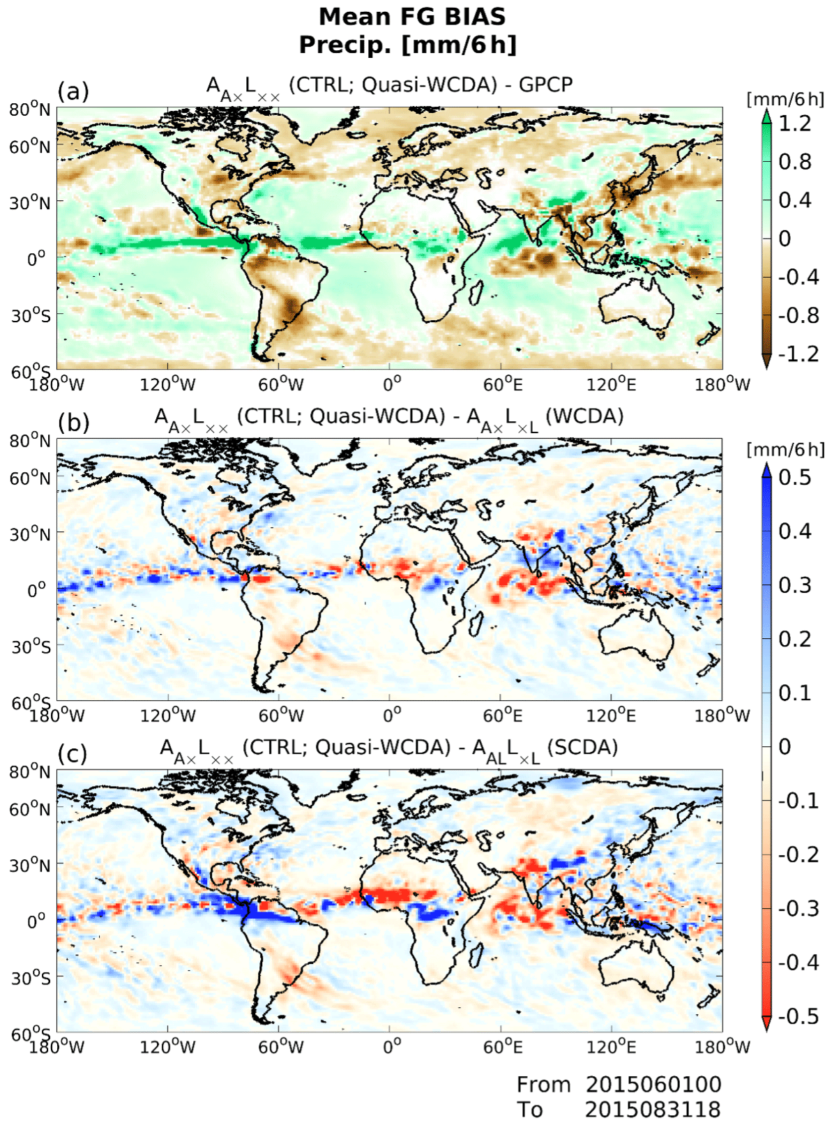
Figure 16Spatial patterns of changes in precipitation (mm 6 h−1) averaged over 3 months from June to August 2014. Panels (a), (b), and (c) show the difference between (CTRL) and GPCP, (CTRL) and (WCDA), and (CTRL) and AALL×L (SCDA), respectively. The green and brown colors in panel (a) represent overestimated and underestimated precipitation values relative to GPCP, and the red and blue colors in panels (b) and (c) represent increased and decreased precipitation values with SM DA, respectively.
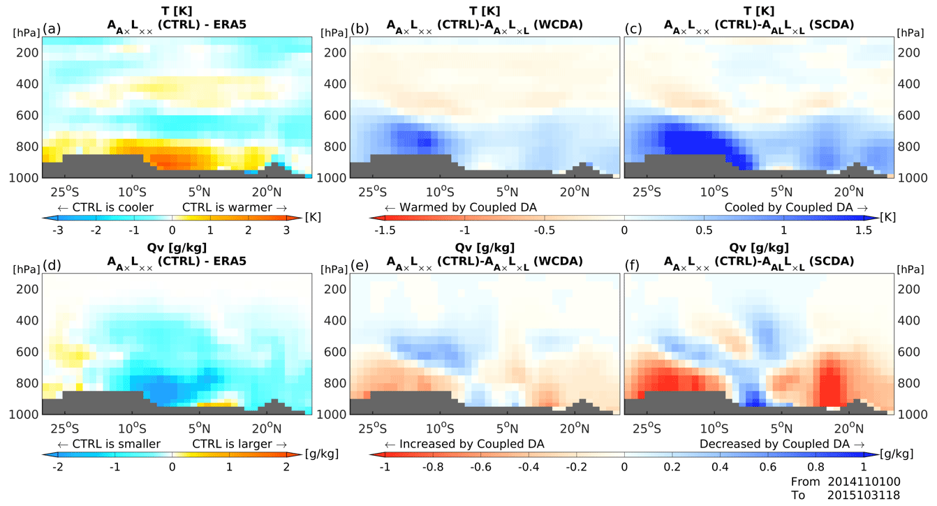
Figure 17Vertical cross-sectional plots of differences in (a–c) temperature (K) and (d–f) water vapor mixing ratio (g kg−1) averaged over 12 months from November 2014 to October 2015 along 20∘ E over the continent of Africa. Panels (a) and (d), (b) and (e), and (c) and (f) show the differences between (CTRL) and the ERA5 reanalysis, (CTRL) and (WCDA), and (CTRL) and AALL×L (SCDA), respectively. The vertical and horizontal axes show the pressure level from 1000 to 100 hPa and the latitude, respectively.
Figure 17 shows vertical cross-sections of forecast biases for temperature and vapor mixing ratio (Qv) relative to ERA5 reanalysis data along 20∘ E over the continent of Africa, averaged over 12 months from November 2014 to October 2015. (CTRL) generally shows a warm temperature bias and a dry humidity bias near the land surface (1000–800 hPa). With the assimilation of SM, (WCDA) and AALL×L (SCDA) show decreases in temperature of the lower troposphere at latitudes where (CTRL) has a warm bias (Fig. 17b and c). Since the vertical layers of NICAM are almost the same as those of the ERA5, the cooling impacts would not be attributed to the difference in vertical resolutions between NICAM and ERA5. (WCDA) propagates the impacts of SM DA for atmospheric variables through the interaction between NICAM and MATSIRO during model time integrations. In addition, AALL×L (SCDA) updates atmospheric variables directly through SM DA, which means AALL×L (SCDA) alters atmospheric variables both directly and indirectly. Therefore, AALL×L (SCDA) lowers temperature too much due to the strong interaction between SM and atmospheric variables (Fig. 17c). Figure 17d shows that most land surface areas have dry Qv biases relative to the ERA5. This corresponds to the locations where (CTRL) exhibits a moist bias against GLDAS (Fig. 4a). As shown in Fig. 4, the coupled DA improves this in those areas, which also leads to an enhancement in the Qv bias in that region. As the moist bias relative to GLDAS in that area is improved through the SM DA, the bias in Qv relative to ERA5 in that area is also improved by coupled assimilation. (WCDA) and AALL×L (SCDA) correct for the bias caused by increased or decreased Qv near the surface using SM DA (Fig. 17e and f). The change for Qv in AALL×L (SCDA) is larger than that in (WCDA). This is because, as previously mentioned, AALL×L (SCDA) makes larger adjustments to atmospheric variables compared to (WCDA).
This study aims to explore the optimal coupled land–atmospheric DA method for improving weather forecasts through the assimilation of hydrological observations. We implement a coupled land–atmospheric DA into the NICAM-MATSIRO model and assimilated SM data from GLDAS. We perform a series of coupled DA experiments, including weakly and strongly coupled DA, and reach the following conclusions.
The assimilation of SM successfully mitigates SM biases. Updating SM by assimilating atmospheric observations can have detrimental impacts on SM, due to spurious error correlations between atmospheric observations and land model variables caused by insufficient ensemble size and the difference in timescale between the atmospheric and land models. In contrast, updating the atmospheric model variables by assimilating SM observations has beneficial impacts on SM, implying that the error correlation between SM observations and atmospheric model variables is more reliable. Consequently, the optimal coupled DA method in this study is AALL×L (SCDA), in which atmospheric and SM data are used to update the atmospheric variables in NICAM, but only SM data are used to update the SM variable in MATSIRO. The results of this study indicate that AALLAL (full-SCDA) is less effective than (WCDA), which is caused by sampling errors and/or insufficient localization of the ensemble background-error covariance matrix. As Penny et al. (2019) have shown, experiments with a simple model to examine several factors in detail, such as the number of ensemble members, the scale of localization, the spread of the ensemble of initial members, and the frequency of coupling intervals, would yield very important information. With adequate settings, such as those proposed by Penny et al. (2019), the experiments with AALLAL (full-SCDA) might give a superior performance. In addition, the difference in dynamical timescales between the atmospheric and land models may possibly have a dominant influence. Using a shorter DA window with more linear cross-domain dynamics could be useful to investigate if this would help improve the impact of the AALLAL (full-SCDA). This will be an important future study. Further, one possible reason that AALLAL (full-SCDA) did not always show optimal results in the current study could be due to the poor and complex physical linkages between the lower troposphere and soil moisture. This problem has reasonably positive effects on the atmospheric field but often results in poor soil moisture analysis. The results presented in this study seem to indicate that this may be the case for AALLAL (full-SCDA).
We demonstrate that precipitation and SM are closely related. Given the seasonal variation in precipitation distribution, the regions that would benefit from updating atmospheric variables using SM data shift accordingly. Assimilating SM provides a proper temperature estimation for the lower troposphere in areas with a dry SM bias and a warm atmospheric bias. This effect occurs because more incoming solar and longwave radiation was converted to latent heat flux and less converted to sensible heat flux with increased SM. However, assimilating SM into atmospheric model variables leads to overcooling effects in regions such as the continents of Africa and Australia. Furthermore, estimating precipitation based on SCDA is beneficial in Africa. Coupled DA has stronger impacts on precipitation forecasts in hotspots where the precipitation field is sensitive to the initial condition of SM.
This study demonstrates the potential for improving SM prediction using the NICAM-LETKF system by assimilating SM in strong coupled DA. SM is an important variable in land surface models, and its improvement can lead to better hydrological predictions such as droughts and floods. However, it is still unclear what atmospheric variables should be updated using each land observation. Therefore, future studies will further investigate the effect of variable localization for other land observations. When updating SM in MATSIRO with atmospheric observations, we obtain unfavorable results due to errors in estimating the error covariance between land model variables and atmospheric observations. The issue is thought to be caused by experimental settings, rather than statistical aspects, due to the poor physical relationships between the lower troposphere and SM. SM behavior is often highly localized due to spatial differences such as soil texture, topography, and vegetation. Therefore, most NWP centers use a point-wise analysis of SM, without considering the horizontal background error covariance between grid points. The 40 ensemble members used in this study are close to the number used in operational NWP centers, but using a larger number of ensembles could lead to useful conclusions by evaluating the differences in performance between WCDA and SCDA. Furthermore, using a large ensemble could be beneficial for understanding variable localization more accurately by improving covariance estimation between components. In this study, land observations are assimilated into the atmospheric model using the same vertical localization scale as the assimilation of atmospheric observations. Using a smaller localization scale in a limited ensemble size could help update atmospheric variables with SM assimilation by reducing errors in the error covariance estimates. Furthermore, while this study uses SM data based on GLDAS, assimilating satellite-derived SM data is an important direction for future research. When actual GCOMW/AMSR-2 satellite observation data are assimilated, the atmospheric field deteriorates significantly due to the assimilation of SM (not shown). This suggests that limitations exist in the data assimilation method used in this study and that technical measures, such as CDF matching preprocessing, may be necessary to assimilate actual observation data successfully. Finally, it is found that a resolution of about 100 km is very coarse to simulate SM accurately. Note that the assimilation of GLDAS pseudo soil moisture data is not a realistic operational setting, as it is likely to have much better spatial and temporal coverage than real satellite observations. When actual observation data are assimilated at this resolution, the representation error becomes large and can cause a problem. In addition to using actual satellite observation data, using higher-resolution models is an important future direction.
This study diagnoses the observation error SD of SM by using innovation statistics (Desroziers et al., 2005). The innovation statistics is given by
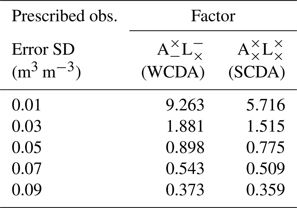
where σo is the observation error SD. Subscript estimation means the estimation by the innovation statistics. The bracket 〈⋅〉 denotes the statistical expectation. Here, we assumed the observation error SD is globally constant and time independent for SM (Rodríguez-Fernández et al., 2019). With NICAM-LETKF, we performed preliminary WCDA and SCDA experiments over 2 months from October to November 2014 and later used 1-month period data for the innovation statistics. Here we introduce a measure factor, given by
where the subscript prescribed denotes the prescribed observation error SD of SM used in the preliminary experiments. If the prescribed SD is optimal, then the diagnosed factor approaches 1.0. Table A1 summarizes the prescribed observation error SD and factor values for five different observation SDs with assimilation of GLDAS SM. As noted by Ménard et al. (2009), when the prescribed observation error SD is too small, the estimated observation error SD is underestimated, whereas large SDs can lead to overestimation. Based on these preliminary experiments, this study set the SM observation error SD at 0.05 (m3 m−3), which gave the factor value closest to 1.0 among the preliminary experiments.
Table A1Observation error SD diagnosed using innovative statistics. “Factor” is the ratio of estimated error SD to the prescribed value (Eq. A2). The diagnostic values from (WCDA) and (SCDA) averaged over 2 months are shown.
All of the data used in this study are stored for 5 years in Chiba University. Due to the large volume of data and limited disk space, data will be shared online upon request (shunji.kotsuki@chiba-u.jp; http://www.data-assimilation.riken.jp/index_e.html, last access: 14 October 2023).
KK and SK developed the experimental system for the parameter estimation, conducted the experiments, and analyzed the results. TM is the PI and directed the research with substantial contribution to the development of this paper.
At least one of the (co-)authors is a member of the editorial board of Nonlinear Processes in Geophysics. The peer-review process was guided by an independent editor, and the authors also have no other competing interests to declare.
Publisher's note: Copernicus Publications remains neutral with regard to jurisdictional claims made in the text, published maps, institutional affiliations, or any other geographical representation in this paper. While Copernicus Publications makes every effort to include appropriate place names, the final responsibility lies with the authors.
The authors thank the members of the Data Assimilation Research Team, RIKEN Center for Computational Science (R-CCS), and JAXA's Precipitation Measuring Mission (PMM) project. This study was partly supported by JAXA (PMM); the Advancement of meteorological and global environmental predictions utilizing observational “Big Data” (Theme 4) to be tackled using the post-K supercomputer of the FLAGSHIP 2020 Project of the Ministry of Education, Culture, Sports, Science and Technology Japan (MEXT); the Initiative for Excellent Young Researchers of MEXT; JST AIP grant number JPMJCR19U2; the Japan Society for the Promotion of Science (JSPS) KAKENHI grant nos. JP18H01549, JP21H04571, JP21H05002, and JP22K18821; JST PRESTO MJPR1924; and IAAR Research Support Program of Chiba University. The study used the Supercomputer for earth Observation, Rockets, and Aeronautics (SORA) at JAXA and the K computer provided by the RIKEN R-CCS (project IDs: ra000015, hp150289, hp160229, hp170246, and hp180062).
This research has been supported by JAXA (PMM); the Advancement of meteorological and global environmental predictions utilizing observational “Big Data” (Theme 4) to be tackled using the post-K supercomputer of the FLAGSHIP 2020 Project of the Ministry of Education, Culture, Sports, Science and Technology Japan (MEXT); the Initiative for Excellent Young Researchers of MEXT; JST AIP (grant no. JPMJCR19U2); the Japan Society for the Promotion of Science (JSPS) KAKENHI (grant nos. JP18H01549, JP21H04571, JP21H05002, and JP22K18821); JST PRESTO (grant no. MJPR1924); and IAAR Research Support Program of Chiba University.
This paper was edited by Wansuo Duan and reviewed by Zheqi Shen and one anonymous referee.
Arakawa, A. and Schubert, W. H.: Interaction of a Cumulus Cloud Ensemble with the Large-Scale Environment, Part I, J. Atmos. Sci., 31, 674–701, https://doi.org/10.1175/1520-0469(1974)031<0674:IOACCE>2.0.CO;2, 1974.
Bateni, S. M. and Entekhabi, D.: Relative efficiency of land surface energy balance components, Water Resour. Res., 48, W04510, https://doi.org/10.1029/2011WR011357, 2012.
Berry, E.: Cloud Droplet Growth by Collection, J. Atmos. Sci., 24, 688–701, https://doi.org/10.1175/1520-0469(1967)024<0688:CDGBC>2.0.CO;2, 1967.
Betts, A. K.: Land-Surface-Atmosphere Coupling in Observations and Models, J. Adv. Model. Earth Syst., 1, 4, https://doi.org/10.3894/JAMES.2009.1.4, 2009.
Bi, H., Ma, J., Zheng, W., and Zeng, J.: Comparison of soil moisture in GLDAS model simulations and in situ observations over the Tibetan Plateau, J. Geophys. Res.-Atmos., 121, 2658–2678, https://doi.org/10.1002/2015JD024131, 2016.
Bindlish, R., Cosh, M. H., Jackson, T. J., Koike, T., Fujii, H., Chan, S. K., Asanuma, J., Berg, A. A., Bosch, D. D., Caldwell, T. G., Collins, C. H., McNairn, H., Martinez-Fernandez, J., Prueger, J. H., Rowlandson, T., Seyfried, M., Starks, P. J., Thibeault, M., Van Der Velde, R., Walker, J. P., and Coopersmith, E. J.: GCOM-W AMSR2 soil moisture product validation using core validation sites, IEEE J. Sel. Top. Appl., 11, 209–219, https://doi.org/10.1109/JSTARS.2017.2754293, 2018.
Bishop, C., Etherton, B., and Majumdar, S.: Adaptive Sampling with the Ensemble Transform Kalman Filter. Part I: Theoretical Aspects, Mon. Weather Rev., 129, 420–436, https://doi.org/10.1175/1520-0493(2001)129<0420:ASWTET>2.0.CO;2, 2001.
Bosilovich, M., Radakovich, J., Silva, A., Todling, R., and Verter, F.: Skin Temperature Analysis and Bias Correction in a Coupled Land-Atmosphere Data Assimilation System, J. Meteorol. Soc. Jpn. II, 85A, 205–228, 2007.
Browne, P.A., de Rosnay, P., Zuo, H., Bennett, A., and Dawson, A.: Weakly Coupled Ocean–Atmosphere Data Assimilation in the ECMWF NWP System, Remote Sens., 11, 234, https://doi.org/10.3390/rs11030234, 2019.
Chen, F., Mitchell, K., Schaake, J., Xue, Y., Pan, H.-L., Koren, V., Duan, Q. Y., Ek, M., and Betts, A.: Modeling of land surface evaporation by four schemes and comparison with FIFE observations, J. Geophys. Res., 101, 7251–7268, https://doi.org/10.1029/95JD02165, 1996.
Dee, D. P.: Bias and data assimilation, Q. J. Roy. Meteor. Soc., 131, 3323–3343, https://doi.org/10.1256/qj.05.137, 2005.
De Lannoy, G. J. M., Reichle, R. H., Houser, P. R., Pauwels, V. R. N., and Verhoest, N. E. C.: Correcting for forecast bias in soil moisture assimilation with the ensemble Kalman filter, Water Resour. Res., 43, W09410, https://doi.org/10.1029/2006WR005449, 2007.
Derber, J. C., Parrish, D. F., and Lord, S. J.: The New Global Operational Analysis System at the National Meteorological Center, Weather Forecast., 6, 538–547, https://doi.org/10.1175/1520-0434(1991)006<0538:TNGOAS>2.0.CO;2, 1991.
de Rosnay, P., Drusch, M., Vasiljevic, D., Balsamo, G., Albergel, C., and Isaksen L.: A simplified extended Kalman filter for the global operational soil moisture analysis at ECMWF, Q. J. Roy. Meteor. Soc., 139, 1199–1213, https://doi.org/10.1002/qj.2023, 2012.
de Rosnay, P., Balsamo, G., Albergel, C., Muñoz-Sabater, J., and Isaksen, L.: Initialisation of Land Surface Variables for Numerical Weather Prediction, Surv. Geophys., 35, 607–621, 2014.
Desroziers, G., Berre, L., Chapnik, B., and Poli, P.: Diagnosis of observation, background and analysis-error statistics in observation space, Q. J. Roy. Meteor. Soc., 131, 3385–3396, https://doi.org/10.1256/qj.05.108, 2005.
Dirmeyer, P. A.: Using a Global Soil Wetness Dataset to Improve Seasonal Climate Simulation, J. Climate, 13, 2900–2922, https://doi.org/10.1175/1520-0442(2000)013<2900:UAGSWD>2.0.CO;2, 2000.
Dirmeyer, P. A. and Halder, S.: Sensitivity of Numerical Weather Forecasts to Initial Soil Moisture Variations in CFSv2, Weather Forecast., 31, 1973–1983, https://doi.org/10.1175/WAF-D-16-0049.1, 2016.
Douville, H. and Chauvin, F.: Relevance of soil moisture for seasonal climate prediction: A preliminary study, Clim. Dynam., 16, 719–736, https://doi.org/10.1007/s003820000080, 2000.
Draper, C. and Reichle, R.H.: Assimilation of Satellite Soil Moisture for Improved Atmospheric Reanalyses, Mon. Weather Rev., 147, 2163–2188, https://doi.org/10.1175/MWR-D-18-0393.1, 2019.
Draper, C. S.: Accounting for Land Model Uncertainty in Numerical Weather Prediction Ensemble Systems: Toward Ensemble-Based Coupled Land–Atmosphere Data Assimilation, J. Hydrometeorol., 22, 2089–2104, 2021.
Drusch, M.: Initializing numerical weather prediction models with satellite-derived surface soil moisture: Data assimilation experiments with ECMWF's Integrated Forecast System and the TMI soil moisture data set, J. Geophys. Res., 112, D03102, https://doi.org/10.1029/2006JD007478, 2007.
Drusch, M. and Viterbo, P.: Assimilation of Screen-Level Variables in ECMWF's Integrated Forecast System: A Study on the Impact on the Forecast Quality and Analyzed Soil Moisture, Mon. Weather Rev., 135, 300–314, https://doi.org/10.1175/MWR3309.1, 2007.
Evensen G.: The Ensemble Kalman Filter: Theoretical formulation and practical implementation, Ocean Dynam., 53, 343–367, https://doi.org/10.1007/s10236-003-0036-9, 2003.
Fairbairn, D., de Rosnay, P., and Browne, P. A.: The New Stand-Alone Surface Analysis at ECMWF: Implications for Land–Atmosphere DA Coupling, J. Hydrometeorol., 20, 2023–2042, 2019.
Frolov, S., Bishop, C., Holt, T., Cummings, D., and Kuhl, D.: Facilitating Strongly Coupled Ocean-Atmosphere Data Assimilation with an Interface Solver, Mon. Weather Rev., 144, 150923131613008, https://doi.org/10.1175/MWR-D-15-0041.1, 2016.
Fujii, Y., Nakaegawa, T., Matsumoto, S., Yasuda, T., Yamanaka, G., and Kamachi, M.: Coupled climate simulation by constraining ocean fields in a coupled model with ocean data, J. Climate, 22, 5541–5557, https://doi.org/10.1175/2009JCLI2814.1, 2009.
Gómez, B., Charlton-Pérez, CL., Lewis, H., and Candy, B.: The Met Office Operational Soil Moisture Analysis System, Remote Sens., 12, 3691, https://doi.org/10.3390/rs12223691, 2020.
Hauser, M., Orth, R., and Seneviratne, S. I.: Investigating soil moisture–climate interactions with prescribed soil moisture experiments: an assessment with the Community Earth System Model (version 1.2), Geosci. Model Dev., 10, 1665–1677, https://doi.org/10.5194/gmd-10-1665-2017, 2017.
Hersbach, H., Bell, B., Berrisford, P., Hirahara, S., Horányi, A., Muñoz-Sabater, J., Nicolas, J., Peubey, C., Radu, R., Schepers, D., Simmons, A., Soci, C., Abdalla, S., Abellan, X., Balsamo, G., Bechtold, P., Biavati, G., Bidlot, J., Bonavita, M., De Chiara, G., Dahlgren, P., Dee, D., Diamantakis, M., Dragani, R., Flemming, J., Forbes, R., Fuentes, M., Geer, A., Haimberger, L., Healy, S., Hogan, R. J., Hólm, E., Janisková, M., Keeley, S., Laloyaux, P., Lopez, P., Lupu, C., Radnoti, G., de Rosnay, P., Rozum, I., Vamborg, F., Villaume, S., and Thépaut, J.-N.: The ERA5 global reanalysis, Q. J. Roy. Meteor. Soc., 146, 1999–2049, https://doi.org/10.1002/qj.3803, 2020.
Honda, T., Miyoshi, T., Lien, G., Nishizawa, S., Yoshida, R., Adachi, S. A., Terasaki, K., Okamoto, K., Tomita, H., and Bessho, K.: Assimilating All-Sky Himawari-8 Satellite Infrared Radiances: A Case of Typhoon Soudelor (2015), Mon. Weather Rev., 146, 213–229, 2018.
Hoover, B. T. and Langland, R. H.: Forecast and observation impact experiments in the Navy Global Environmental Model with assimilation of ECWMF analysis data in the global domain, J. Meteorol. Soc. Jpn., 95, 369–389, https://doi.org/10.2151/jmsj.2017-023, 2017.
Hunt, B. R., Kostelich, E. J., and Szunyogh, I.: Efficient data assimilation for spatiotemporal chaos: A local ensemble transform Kalman filter, Phys. D, 230, 112–126, https://doi.org/10.1016/j.physd.2006.11.008, 2007.
Kang, J.-S., Kalnay, E., Liu, J., Fung, I., Miyoshi, T., and Ide, K.: “Variable localization” in an ensemble Kalman filter: Application to the carbon cycle data assimilation, J. Geophys. Res., 116, D09110, https://doi.org/10.1029/2010JD014673, 2011.
Kikuchi, K., Kodama, C., Nasuno, T., Nakano, M., Miura, H., Satoh, M., Noda, A. T., and Yamada, Y.: Tropical intraseasonal oscillation simulated in an AMIP-type experiment by NICAM, Clim. Dynam., 48, 2507–2528, https://doi.org/10.1007/s00382-016-3219-z, 2017.
Kodama, C., Yamada, Y., Noda, A. T., Kikuchi, K., Kajikawa, Y., Nasuno, T., Tomita, T., Yamaura, T., Takahashi, T. G., Hara, M., Kawatani, Y., Satoh, M., and Sugi, M.: A 20-year climatology of a NICAM AMIP-type simulation, J. Meteorol. Soc. Jpn., 93, 393–424, https://doi.org/10.2151/jmsj.2015-024, 2015.
Koren, V., Schaake, J., Mitchell, K., Duan, Q. Y., Chen, F., and Baker, J. M.: A parameterization of snowpack and frozen ground intended for NCEP weather and climate models, J. Geophys. Res., 104, 19569–19585, https://doi.org/10.1029/1999JD900232, 1999.
Koster, R. D., Dirmeyer, P. A., Guo, Z., Bonan, G., Chan, E., Cox, P., Gordon, C. T., Kanae, S., Kowalczyk, E., Lawrence, D., Liu, P., Lu, C. H., Malyshev, S., McAvaney, B., Mitchell, K., Mocko, D., Oki, T., Oleson, K., Pitman, A., Sud, Y. C., Taylor, C. M., Verseghy, D., Vasic, R., Xue, Y., and Yamada, T.: Regions of strong coupling between soil moisture and precipitation, Science, 305, 1138–1140, https://doi.org/10.1126/science.1100217, 2004.
Kotsuki, S., Miyoshi, T., Terasaki, K., Lien, G.-Y., and Kalnay, E.: Assimilating the global satellite mapping of precipitation data with the Nonhydrostatic Icosahedral Atmospheric Model (NICAM), J. Geophys. Res., 122, 631–650, https://doi.org/10.1002/2016JD025355, 2017a.
Kotsuki, S., Ota, Y., and Miyoshi, T.: Adaptive covariance relaxation methods for ensemble data assimilation: experiments in the real atmosphere, Q. J. Roy. Meteor. Soc., 143, 2001–2015, https://doi.org/10.1002/qj.3060, 2017b.
Kotsuki, S., Terasaki, K., Yashiro, H., Tomita, H., Satoh, M., and Miyoshi, T.: Online Model Parameter Estimation with Ensemble Data Assimilation in the Real Global Atmosphere: A Case with the Nonhydrostatic Icosahedral Atmospheric Model (NICAM) and the Global Satellite Mapping of Precipitation Data, J. Geophys. Res., 123, 7375–7392, https://doi.org/10.1029/2017JD028092, 2018.
Kotsuki, S., Kurosawa, K., and Miyoshi, T.: On the properties of ensemble forecast sensitivity to observations, Q. J. Roy. Meteor. Soc., 145, 1897–1914, https://doi.org/10.1002/qj.3534, 2019a.
Kotsuki, S., Kurosawa, K., Otsuka, S., Terasaki, K., and Miyoshi, T.: Global Precipitation Forecasts by Merging Extrapolation-based Nowcast and Numerical Weather Prediction with Locally-optimized Weights, Weather Forecast., 34, 701–714, https://doi.org/10.1175/WAF-D-18-0164.1, 2019b.
Kotsuki, S., Terasaki, K., Kanemaru, K., Satoh, M., Kubota, T., and Miyoshi, T.: Predictability of Record-Breaking Rainfall in Japan in July 2018: Ensemble Forecast Experiments with the Near-real-time Global Atmospheric Data Assimilation System NEXRA, SOLA, 15A, 1–7, https://doi.org/10.2151/sola.15A-001, 2019c.
Laloyaux, P., Balmaseda, M., Dee, D., Mogensen, K., and Janssen, P.: A coupled data assimilation system for climate reanalysis, Q. J. Roy. Meteor. Soc., 142, 65–78, https://doi.org/10.1002/qj.2629, 2016.
Lea, D. J., Mirouze, I., Martin, M. J., King, R. R., Hines, A., Walters, D., and Thurlow, M.: Assessing a New Coupled Data Assimilation System Based on the Met Office Coupled Atmosphere–Land–Ocean–Sea Ice Model, Mon. Weather Rev., 143, 4678–4694, https://doi.org/10.1175/MWR-D-15-0174.1, 2015.
Lin, L. and Pu, Z.: Examining the Impact of SMAP Soil Moisture Retrievals on Short-Range Weather Prediction under Weakly and Strongly Coupled Data Assimilation with WRF-Noah, Mon. Weather Rev., 147, 4345–4366, https://doi.org/10.1175/MWR-D-19-0017.1, 2019.
Lin, L. and Pu, Z.: Improving Near-Surface Short-Range Weather Forecasts Using Strongly Coupled Land-Atmosphere Data Assimilation with GSI-EnKF, Mon. Weather Rev., 148, 2863–2888, https://doi.org/10.1175/MWR-D-19-0370.1, 2020.
Mahfouf, J., Viterbo, P., Douville, H., Beljaars, A., and Saarinen, S.: A Revised land-surface analysis scheme in the Integrated Forecasting System, ECMWF Newsletter, Summer–Autumn, 2000.
Ménard, R., Yang, Y., and Rochon, Y.: Convergence and stability ofestimated error variances derived from assimilation residuals in observa-tion space, Proceedings of ECMWF Workshop on Diagnostics of Data Assimilation System Performance, 15–17 June 2009, Reading, UK, 2009.
Miyoshi, T. and Yamane, S.: Local Ensemble Transform Kalman Filtering with an AGCM at a T159/L48 Resolution, Mon. Weather Rev., 135, 3841–3861, https://doi.org/10.1175/2007MWR1873.1, 2007.
Penny, S. and Hamill, T.: Coupled Data Assimilation for Integrated Earth System Analysis and Prediction, B. Am. Meteorol. Soc., 98, ES169–ES172, https://www.jstor.org/stable/26243775 (last access: 14 October 2023), 2017.
Penny, S. G., Bach, E., Bhargava, K., Chang, C.-C., Da, C., Sun, L., and Yoshida, T.: Strongly coupled data assimilation in multiscale media: Experiments using a quasi-geostrophic coupled model, J. Adv. Model. Earth Syst., 11, 1803–1829, 2019.
Reichle, R. H. and Koster, R. D.: Bias reduction in short records of satellite soil moisture, Geophys. Res. Lett., 31, L19501, https://doi.org/10.1029/2004GL020938, 2004.
Reichle, R. H., McLaughlin, D. B., and Entekhabi, D.: Hydrologic Data Assimilation with the Ensemble Kalman Filter, Mon. Weather Rev., 130, 103–114, https://doi.org/10.1175/1520-0493(2002)130<0103:HDAWTE>2.0.CO;2, 2002.
Reichle, R. H., Kumar, S. V., Mahanama, S. P. P., Koster, R. D., and Liu, Q.: Assimilation of Satellite-Derived Skin Temperature Observations into Land Surface Models, J. Hydrometeorol., 11, 1103–1122, 2010.
Rodell, M., Houser, P. R., Jambor, U., Gottschalck, J., Mitchell, K., Meng, C., Arsenault, K., Cosgrove, B., Radakovich, J., Bosilovich, M., Entin, J. K., Walker, J. P., Lohmann, D., and Toll, D.: The Global Land Data Assimilation System, B. Am. Meteorol. Soc., 85, 381–394, https://doi.org/10.1175/BAMS-85-3-381, 2004.
Rodríguez-Fernández, N., de Rosnay, P., Albergel, C., Richaume, P., Aires, F., Prigent, C., and Kerr, Y.: SMOS Neural Network Soil Moisture Data Assimilation in a Land Surface Model and Atmospheric Impact, Remote Sens., 11, 1334, https://doi.org/10.3390/rs11111334, 2019.
Santanello, J. A., Lawston, P., Kumar, S., and Dennis, E.: Understanding the impacts of soil moisture initial conditions on NWP in the context of land–atmosphere coupling, J. Hydrometeorol., 20, 793–819, https://doi.org/10.1175/JHM-D-18-0186.1, 2019.
Satoh, M., Matsuno, T., Tomita, H., Miura, H., Nasuno, T., and Iga, S.: Nonhydrostatic icosahedral atmospheric model (NICAM) for global cloud resolving simulations, J. Comput, Phys., 227, 3486–3514, https://doi.org/10.1016/j.jcp.2007.02.006, 2008.
Satoh, M., Tomita, H., Yashiro, H., Miura, H., Kodama, C., Seiki, T., Noda, A., Yamada, Y., Goto, D., Sawada, M., Miyoshi, T., Niwa, Y., Hara, M., Ohno, Y., Iga, S., Arakawa, T., Inoue, T., and Kubokawa, H.: The Non-hydrostatic Icosahedral Atmospheric Model: description and development, Prog. Earth Planet. Sci., 1, 18, https://doi.org/10.1186/s40645-014-0018-1, 2014.
Sawada, Y., Nakaegawa, T., and Miyoshi, T.: Hydrometeorology as an inversion problem: Can river discharge observations improve the atmosphere by ensemble data assimilation?, J. Geophys. Res.-Atmos., 123, 848–860, https://doi.org/10.1002/2017JD027531, 2018.
Sluka, T. C., Penny, S. G., Kalnay, E., and Miyoshi, T.: Assimilating atmospheric observations into the ocean using strongly coupled ensemble data assimilation, Geophys. Res. Lett., 43, 752–759, https://doi.org/10.1002/2015GL067238, 2016.
Sugiura, N., Awaji, T., Masuda, S., Mochizuki, T., Toyoda, T., Miyama, T., Igarashi, H., and Ishikawa, Y.: Development of a four-dimensional variational coupled data assimilation system for enhanced analysis and prediction of seasonal to interannual climate variations, J. Geophys. Res., 113, C10017, https://doi.org/10.1029/2008JC004741, 2008.
Suzuki, K., Zupanski, M., and Zupanski, D.: A case study involving single observation experiments performed over snowy Siberia using a coupled atmosphere-land modelling system, Atmos. Sci. Lett, 18, 106–111, https://doi.org/10.1002/asl.730, 2017.
Takata, K., Emori, S., and Watanabe, T.: Development of the minimal advanced treatments of surface interaction and runoff, Global Planet. Chang., 38, 209–222, https://doi.org/10.1016/S0921-8181(03)00030-4, 2003.
Tang, Q., Mu, L., Goessling, H. F., Semmler, T., and Nerger, L.: Strongly coupled data assimilation of ocean observations into an ocean-atmosphere model, Geophys. Res. Lett., 48, e2021GL094941, https://doi.org/10.1029/2021GL094941, 2021.
Terasaki, K. and Miyoshi, T.: Assimilating AMSU-A Radiances with the NICAM-LETKF, J. Meteorol. Soc. Jpn., 95, 433–446, https://doi.org/10.2151/jmsj.2017-028, 2017.
Terasaki, K., Sawada, M., and Miyoshi, T.: Local Ensemble Transform Kalman Filter Experiments with the Nonhydrostatic Icosahedral Atmospheric Model NICAM, SOLA, 11, 23–26, https://doi.org/10.2151/sola.2015-006, 2015.
Terasaki, K., Kotsuki, S., and Miyoshi, T.: Multi-year analysis using the NICAM-LETKF data assimilation system, SOLA, 15, 41–46, https://doi.org/10.2151/sola.2019-009, 2019.
Whitaker, J. S. and Hamill, T. M.: Evaluating Methods to Account for System Errors in Ensemble Data Assimilation, Mon. Weather Rev., 140, 3078–3089, https://doi.org/10.1175/MWR-D-11-00276.1, 2012.
Zhang, S., Harrison, M. J., Rosati, A., and Wittenberg, A.: System Design and Evaluation of Coupled Ensemble Data Assimilation for Global Oceanic Climate Studies, Mon. Weather Rev.,135, 3541–3564, https://doi.org/10.1175/MWR3466.1, 2007.