Toward a multivariate formulation of the parametric Kalman filter assimilation: application to a simplified chemical transport model

This contribution explores a new approach to forecasting multivariate covariances for atmospheric chemistry through the use of the parametric Kalman filter (PKF). In the PKF formalism, the error covariance matrix is modellized by a covariance model relying on parameters, for which the dynamics are then computed. The PKF has been previously formulated in univariate cases, and a multivariate extension for chemical transport models is explored here. This contribution focuses on the situation where the uncertainty is due to the chemistry but not due to the uncertainty of the weather. To do so, a simplified two-species chemical transport model over a 1D domain is introduced, based on the non-linear Lotka–Volterra equations, which allows us to propose a multivariate pseudo covariance model. Then, the multivariate PKF dynamics are formulated and their results are compared with a large ensemble Kalman filter (EnKF) in several numerical experiments. In these experiments, the PKF accurately reproduces the EnKF. Eventually, the PKF is formulated for a more complex chemical model composed of six chemical species (generic reaction set). Again, the PKF succeeds at reproducing the multivariate covariances diagnosed on the large ensemble.

1 Introduction

Data assimilation aims to provide an estimation of the true state of a system. This estimation, called the analysis, is a compromise between the forecast of the state and the available observations. The optimal combination of the forecast and the observations relies on their respective error covariance matrices as given by the Kalman filter equations (Kalman, 1960). The accuracy of the analysis is directly related to the quality of these two matrices.

In atmospheric chemistry applications, the system to study is the concentration of multiple chemical species in the atmosphere. In most cases, chemical transport models (CTMs) are used to forecast the concentrations, such as the operational Model Of atmospheric Chemistry At larGE scale (MOCAGE) used in Météo-France (Josse et al., 2004). CTMs make predictions based on the transport by the wind (the fields are provided by numerical weather prediction (NWP) models) and the chemical interactions of the species (Hauglustaine et al., 1998) and take into account multiple other important processes, e.g. the diffusion, the emissions, the deposition, or the interaction with clouds. However, in CTMs, chemistry does not influence the meteorology, which is of course a crude approximation of the true atmosphere. The advantage of a CTM is that it allows air quality prediction at a low numerical cost and is used in several operational centres. For instance, the Copernicus Atmosphere Monitoring Service (CAMS) regional air quality production (https://atmosphere.copernicus.eu/cams-european-air-quality-ensemble-forecasts-welcomes-two-new-state-art-models, associated with CAMS2.40 at https://confluence.ecmwf.int/display/CKB/CAMS+Regional%3A+European+air+quality+analysis+and+forecast+data+documentation; see here for a scientific description – last access to web references: 15 March 2023), which forecasts daily a multi-model ensemble of 11 members that covers the following 4 d, is performed from the integration of 11 models, of which 10 are CTMs. Note that each member of the ensemble relies on its own data assimilation system for providing its surface analysis, while all the models process the same set of surface observations, and all the model forecasts are based on the same meteorological forcings from European Centre for Medium-Range Weather Forecasts (ECMWF) high-resolution weather forecasts. In particular, members of the CAMS multi-model ensemble are not used within an EnKF to provide its own assimilation system.

In this context, the forecast-error covariance matrix contains the correlations of the forecast errors within and between the chemical species. In multivariate covariance modelling applied in meteorology, these correlations are respectively denoted as auto-correlations and cross-correlations (Derber and Bouttier, 1999). Accurately describing the auto-correlation and cross-correlation is a key component in improving the overall quality of the analysis. Indeed, strong correlations exist between different chemical species, and the analysis could benefit from them: an observation for a given species might also correct other concentrations and reduce their error amplitude at the same time. Note that, in operational applications, chemical species are often assimilated separately; for example, in CAMS 2.40, the univariate 3D variational data assimilation (3DVar) system of MOCAGE is used for the assimilation of ozone, nitrogen dioxide, sulfur dioxide, and fine particulate matter PM_2.5 and PM₁₀ (following a configuration similar to the one used for Monitoring Atmospheric Composition and Climate: Interim Implementation (MACII) detailed by Marécal et al., 2015). Note also that simplifications are often introduced to represent a flow dependency of the background term. For example, in several studies using MOCAGE, the 3DVar background error standard deviations are specified as a percentage of the first-guess field (El Amraoui et al., 2020; El Aabaribaoune et al., 2021; Peiro et al., 2018) – which is very different from the forecast-error variance in an ensemble Kalman filter (EnKF) that results from the ensemble estimation and the dynamics of the uncertainty along the previous analysis and forecast cycles.

However, the estimation and the modelling of multivariate covariances in air quality are complex topics (Emili et al., 2016). However, this is not specific to air quality, and two main approaches are found in data assimilation. The first one relies on balance operators and has been introduced in variational data assimilation. These balance operators establish a relation between the state variables and allow for the modelling of cross-covariances from the design of univariate covariances. Such operators exist in numerical weather prediction (Derber and Bouttier, 1999; Fisher, 2003) and for the ocean (Weaver et al., 2006), but as far as we know, no balance operators are used in atmospheric chemistry applications. The second approach relies on the ensemble method (Evensen, 2009), where an ensemble of forecasts is used to estimate the multivariate covariance matrix (Coman et al., 2012). The ensemble method offers a flow-dependent estimation of the error statistics and leads to a practical implementation of the Kalman filter, which is the EnKF (Evensen, 1994). The EnKF applies to a wide range of problems, from a simple Lorenz-63 model (Lorenz, 1963) to the numerical prediction of the atmosphere or the ocean. At the same time, this advantage may be seen as a limitation: the EnKF does not necessarily take advantage of the particular set of equations of a problem, e.g. the continuity of physical fields, which leads to simplification not available in the usual matrix formulation of the EnKF equations. Moreover, the ensemble method presents some drawbacks. For instance, since the estimation often relies on a small ensemble, the statistical estimations are polluted by a spurious sampling noise which requires the introduction of filtering (Berre et al., 2007) and localization (Houtekamer and Mitchell, 1998, 2001). In air quality, it may be preferable to set the ensemble estimation of the multivariate correlation to zero to avoid polluting the resulting analysis state (Tang et al., 2011; Gaubert et al., 2014), except at the globe's surface (Eben et al., 2005) or when the chemical species are strongly correlated (Miyazaki et al., 2012). Note that additional treatments can be required as inflation of the variance in order to represent effects of model errors (Anderson and Anderson, 1999; Whitaker and Hamill, 2003). As another drawback, the numerical computation of the EnKF is costly since it relies on the several time integrations of a numerical model, which are often computed in parallel at lower resolution.

Recently, a new approximation of the Kalman filter (KF) was introduced, the parametric Kalman filter (PKF), where the error covariance matrices are approximated by a covariance model fitted with a set of parameters, e.g. the grid-point variance and the local anisotropy (Pannekoucke et al., 2016). In the PKF, the dynamics of the parameters are described all along the forecast and analysis steps of the assimilation cycle (Pannekoucke, 2021a). This approach does not rely on ensembles, and the dynamics of the parameters are deduced from the partial differential equations that govern the physical system. Hence, the PKF opens the way to understanding the physics of uncertainties. However, the construction of the parameter dynamics is the most difficult part for the design of the PKF. When the parameters are the variance and the local error-correlation anisotropy, a systematic formalism for deducing the PKF's equations based on a Reynolds decomposition (or Reynolds averaging technique; see e.g. Lesieur, 2008, chap. 4) has been introduced, associated with a Python package, SymPKF (Pannekoucke and Arbogast, 2021; Pannekoucke, 2021b), and is based on the Python computer algebra system Sympy (Meurer et al., 2017). However, modelling the physics of uncertainties often comes with closure problems. To alleviate this issue, another numerical framework, PDE-Netgen, has been introduced to be able to close problems using a deep-learning approach (Pannekoucke and Fablet, 2020; Pannekoucke, 2020).

Applying the PKF approach for CTMs is attractive because the parametric dynamics are known for the transport equations (Cohn, 1993; Pannekoucke et al., 2018), and this leads to a better understanding of the forecast-error covariance dynamics, e.g. a better understanding of the model-error covariance due to the numerical integration (Pannekoucke et al., 2021) and the loss of variance which appears in the EnKF (Ménard et al., 2021). Moreover, an application of the PKF was recently proposed for the assimilation of Greenhouse Gases Observing Satellite (GOSAT) methane in the hemispheric Community Multiscale Air Quality (CMAQ) model (Voshtani et al., 2022a, b), showing the potential of the PKF in nearly operational applications where only the error variance evolved. Compared to specifying the background variance as a percentage of the first guess, as mentioned above for the MOCAGE assimilation, the PKF could provide a flow dependence more consistent with the KF theoretical framework but without the numerical cost of using an ensemble as with an EnKF.

While the PKF has been formulated for univariate statistics, a first attempt at multivariate statistics has been proposed based on the balance operator approach (Pannekoucke, 2021a). However, applying such a balance operator is a challenge for chemical reactions where no simple relation exists as the geostrophic balance in weather forecasting. Hence, the aim of this contribution is to explore how to extend the univariate PKF to a multivariate formulation adapted to CTMs. To do so, a multivariate covariance model adapted to air quality prediction is first proposed, and then it is validated by a twin experiment based on an EnKF using a large ensemble.

This contribution only focuses on the uncertainty dynamics due to the chemistry without accounting for the part of the uncertainty of the weather: for example, we do not take into account the uncertainty of the wind that transports the chemical species.

The paper is organized as follows. Section 2 recalls basic concepts in data assimilation with the formalism of the Kalman filter and its parametric approximation in univariate statistics. Then, in Sect. 3, a simplified two-species multivariate CTM is introduced for which a multivariate parametric assimilation is first proposed and then validated based on a comparison with an ensemble approach. A six-species chemical scheme is considered in Sect. 4 to evaluate the PKF multivariate forecast in a more complex context. The conclusions of the contribution are given in Sect. 5.

2 Background on the parametric Kalman filter

The PKF is a recent implementation of the Kalman filter where the covariance matrices are approximated by some covariance model. For the sake of consistency, this section first recaps the basics of the Kalman filter, and then it recalls the diagnosis of the covariance matrix in large-dimension and covariance models to introduce the formalism of the PKF in univariate statistics. The section ends with a numerical example of interest for air quality that illustrates the PKF.

2.1 Analysis and forecast step in the Kalman filter

Here we consider a system whose state is denoted by 𝒳 and governed by the evolution equation

$$\begin{array}{}\text{(1)}& {\partial }_t\mathcal{X}=\mathcal{M}\left(\mathcal{X}\right).\end{array}$$

Time integration from a time t_q to a time t_q+1 of the dynamics in Eq. (1) defines the propagator ${\mathcal{M}}_{t_{q+\mathrm{1}}\leftarrow t_q}$, which maps a state 𝒳(t_q) to the prediction of Eq. (1), $\mathcal{X}\left(t_{q+\mathrm{1}}\right)={\mathcal{M}}_{t_{q+\mathrm{1}}\leftarrow t_q}\mathcal{X}\left(t_q\right)$. In geophysics, 𝒳 stands for the multivariate fields that represent the state of the ocean, the atmosphere, or chemical species concentration for air quality. The dynamics ℳ are then given by a system of partial differential equations. After spatial discretization, ℳ becomes a system of ordinary differential equations, and 𝒳 is a vector of dimension n. Thereafter, 𝒳 can be seen either as a collection of continuous fields with dynamics given by Eq. (1) or a discrete vector of dynamics in the discretized version of Eq. (1).

Because of the spatio-temporal sparsity of observations, modelling, and chaotic amplification of initial error in forecast and measurement errors, the exact actual state at a time t=t_q, ${\mathcal{X}}_q^{\mathrm{t}}$, is unknown.

Data assimilation aims to provide the analysis state, ${\mathcal{X}}_q^{\mathrm{a}}$, which is an estimation of ${\mathcal{X}}_q^{\mathrm{t}}$ performed from the observations and the forecast state. The analysis state is decomposed into ${\mathcal{X}}_q^{\mathrm{a}}={\mathcal{X}}_q^{\mathrm{t}}+{\mathit{\epsilon }}_q^{\mathrm{a}}$, where ${\mathit{\epsilon }}_q^{\mathrm{a}}$ is the analysis error, which is modelled as a random error of the zero mean and covariance matrix ${\mathbf{P}}_q^{\mathrm{a}}=\mathbb{E}\left({\mathit{\epsilon }}_q^{\mathrm{a}}({\mathit{\epsilon }}_q^{\mathrm{a}}{)}^{\mathrm{T}}\right)$, with 𝔼 (or its shorthand $\stackrel{\mathrm{‾}}{\cdot }$) the expectation operator and ^T the transpose operator. This analysis state ${\mathcal{X}}_q^{\mathrm{a}}$ can be obtained by combining the forecast state ${\mathcal{X}}_q^{\mathrm{f}}$ and the observations ${\mathcal{Y}}_q^{\mathrm{obs}}$. Similarly to the analysis state, the forecast and the observations can be written as ${\mathcal{X}}_q^{\mathrm{f}}={\mathcal{X}}_q^{\mathrm{t}}+{\mathit{\epsilon }}_q^{\mathrm{f}}$ and ${\mathcal{Y}}_q^{\mathrm{obs}}=Y_q^{\mathrm{t}}+{\mathit{\epsilon }}_q^{\mathrm{obs}}$, introducing the forecast (observation) error ${\mathit{\epsilon }}_q^{\mathrm{f}}$ (${\mathit{\epsilon }}_q^{\mathrm{obs}}$), both modelled as random errors of zero-mean and covariance matrices ${\mathbf{P}}_q^{\mathrm{f}}=\mathbb{E}\left({\mathit{\epsilon }}_q^{\mathrm{f}}({\mathit{\epsilon }}_q^{\mathrm{f}}{)}^{\mathrm{T}}\right)$ and ${\mathbf{R}}_q=\mathbb{E}\left({\mathit{\epsilon }}_q^{\mathrm{obs}}({\mathit{\epsilon }}_q^{\mathrm{obs}}{)}^{\mathrm{T}}\right)$ respectively. In the case when the dynamic of 𝒳^t is assumed to be linear, replacing ℳ with its matrix version M in Eq. (1), and when the errors are Gaussian, uncorrelated in time, and errors between observations and forecast are independent, the KF's equations describe the evolution of the uncertainty over time (Kalman, 1960).

The process of estimating the analysis state from a forecast and some observations is called the analysis step. The forecast-error covariance matrix denoted by ${\mathbf{P}}_q^{\mathrm{f}}$ and the observation error covariance matrix R_q associated respectively with ${\mathcal{X}}_q^{\mathrm{f}}$ and ${\mathcal{Y}}_q^{\mathrm{obs}}$ are used to produce the optimal estimation (analysis) ${\mathcal{X}}_q^{\mathrm{a}}$ of ${\mathcal{X}}_q^{\mathrm{t}}$ and the associated analysis-error covariance matrix ${\mathbf{P}}_q^{\mathrm{a}}$. The equations of this procedure are

$$\begin{array}{}\text{(2a)}& {\displaystyle }& {\displaystyle }{\mathcal{X}}_q^{\mathrm{a}}={\mathcal{X}}_q^{\mathrm{f}}+{\mathbf{K}}_q\left({\mathcal{Y}}_q^{\mathrm{obs}}-{\mathbf{H}}_q{\mathcal{X}}_q^{\mathrm{f}}\right),\text{(2b)}& {\displaystyle }& {\displaystyle }{\mathbf{P}}_q^{\mathrm{a}}=\left({\mathbf{I}}_n-{\mathbf{K}}_q{\mathbf{H}}_q\right){\mathbf{P}}_q^{\mathrm{f}},\end{array}$$

where ${\mathbf{K}}_q={\mathbf{P}}_q^{\mathrm{f}}{\mathbf{H}}_q^{\mathrm{T}}{\left({\mathbf{H}}_q{\mathbf{P}}_q^{\mathrm{f}}{\mathbf{H}}_q^{\mathrm{T}}+{\mathbf{R}}_q\right)}^{-\mathrm{1}}$ is the Kalman gain matrix, with H_q the linear observation operator that maps the state vector into the observation space, ${\mathbf{P}}_q^{\mathrm{a}}$ the analysis-error covariance matrix, and I_n the identity matrix in dimension n.

Next, the forecast step pushes the uncertainty forward in time. The analysis state ${\mathcal{X}}_q^{\mathrm{a}}$ is propagated using the linear dynamics M to obtain the forecast ${\mathcal{X}}_{q+\mathrm{1}}^{\mathrm{f}}$ at time t_q+1, leading to an estimation of the true state system 𝒳^t(t_q+1). The Gaussian error statistics for this forecast are given by the Kalman filter forecast steps

$$\begin{array}{}\text{(3a)}& {\displaystyle }& {\displaystyle }{\mathcal{X}}_{q+\mathrm{1}}^{\mathrm{f}}={\mathbf{M}}_{q+\mathrm{1}\leftarrow q}{\mathcal{X}}_q^{\mathrm{a}},\text{(3b)}& {\displaystyle }& {\displaystyle }{\mathbf{P}}_{q+\mathrm{1}}^{\mathrm{f}}={\mathbf{M}}_{q+\mathrm{1}\leftarrow q}{\mathbf{P}}_q^{\mathrm{a}}{\left({\mathbf{M}}_{q+\mathrm{1}\leftarrow q}\right)}^{\mathrm{T}}+{\mathbf{Q}}_q,\end{array}$$

where Q_q is the model-error covariance matrix. Thereafter, no model error is considered: i.e. Q is zero.

While the Kalman filter formalism is based on simple vector algebra equations, it is not easy to understand the statistical content of the error covariances, which would require representing each covariance function and exploring their temporal evolution. Fortunately, simple diagnosis can be introduced to summarize the statistical relationship between points in the geographic domain. In turn, these diagnostics can be used as parameters of covariance models, as detailed now.

2.2 Diagnosis and modelling of the covariance matrix in a large dimension

In data assimilation, two diagnoses for the error covariance matrices are often introduced: the variance field and the anisotropy of the correlation functions which correspond to the principal axes of the spatial correlation. These diagnoses are used for the description of the forecast-error covariance matrix.

The forecast-error variance field, V^f, is defined by V^f(x)=𝔼((ε^f(x))²), where x denotes the coordinate of a grid point. The variance field also corresponds to the diagonal of P^f. The field of variance characterizes the magnitude of the error at a given position.

When the forecast error is a differential random field, the anisotropy of the correlation is characterized by the so-called local forecast-error metric tensor g^f(x) that appears in the Taylor expansion of the correlation function (Daley, 1991)

$$\begin{array}{}\text{(4)}& {\mathit{\rho }}^{\mathrm{f}}(\mathit{x},\mathit{x}+\mathit{\delta }\mathit{x})\approx \mathrm{1}-{\displaystyle \frac{\mathrm{1}}{\mathrm{2}}}\left|\right|\mathit{\delta }\mathit{x}|{|}_{{\mathit{g}}^{\mathrm{f}}\left(\mathit{x}\right)}^{\mathrm{2}},\end{array}$$

where $\left|\right|\cdot |{|}_{\mathit{g}}$ stands for the Euclidean norm associated with a metric g and defined from $\left|\right|\mathit{x}|{|}_{\mathit{g}}^{\mathrm{2}}={\mathit{x}}^T\mathit{g}\mathit{x}$. The local metric tensor g^f(x) is a symmetric positive-definite matrix that prevents the correlation value from being larger than one. There is one local metric tensor at each grid location x. The metric tensor is related to the statistics of the random field ε^f according to the formula (Berre et al., 2007)

$$\begin{array}{}\text{(5)}& {\mathit{g}}_{ij}^{\mathrm{f}}\left(\mathit{x}\right)=\mathbb{E}\left[{\partial }_{{\mathit{x}}^i}\left({\displaystyle \frac{{\mathit{\epsilon }}^{\mathrm{f}}}{{\mathit{\sigma }}^{\mathrm{f}}}}\right){\partial }_{{\mathit{x}}^j}\left({\displaystyle \frac{{\mathit{\epsilon }}^{\mathrm{f}}}{{\mathit{\sigma }}^{\mathrm{f}}}}\right)\right]\left(\mathit{x}\right),\end{array}$$

where ${\mathit{\sigma }}^{\mathrm{f}}=\sqrt{V^{\mathrm{f}}}$ is the forecast-error standard deviation and where x_i denotes the coordinate functions associated with the coordinate system x.

In practice, the direction of the largest correlation anisotropy corresponds to the principal axis of the smallest eigenvalue for the metric tensor: the metric tensor is contravariant. It is thus useful to introduce the local aspect tensor (Purser et al., 2003), whose geometry goes as the correlation and is defined as the inverse of the metric tensor:

$$\begin{array}{}\text{(6)}& {\mathit{s}}^{\mathrm{f}}\left(\mathit{x}\right)={\left({\mathit{g}}^{\mathrm{f}}\left(\mathit{x}\right)\right)}^{-\mathrm{1}},\end{array}$$

where the superscript “⁻¹” denotes the matrix inverse. Note that, in a 1D domain, the square root of s is homogeneous to a length, leading to the so-called length scale $l=\sqrt{s}$, which is often introduced in diagnoses.

One of the motivations behind the diagnosis of the variance and the local anisotropy tensor is that they can be used as parameters of covariance models, the VLATcov models (Pannekoucke, 2021a). For instance, for the covariance model based on a diffusion equation (Weaver and Courtier, 2001), the anisotropy tensor has been used as a proxy for setting the heterogeneous diffusion tensor field of the covariance model based on a heterogeneous diffusion equation (Pannekoucke and Massart, 2008; Mirouze and Weaver, 2010). This covariance model is used in variation data assimilation to generate heterogeneous covariances where correlation functions vary between grid points. While there is no analytical expression for the covariance functions based on the diffusion operator, analytical heterogeneous VLATcov models exist, for instance the heterogeneous Gaussian-like covariance model

$$\begin{array}{}\text{(7)}& \begin{array}{rl}& {\mathbf{P}}^{\mathtt{\text{he.gauss}}}(V,\mathit{s})(\mathit{x},\mathit{y})=\sqrt{V\left(\mathit{x}\right)V\left(\mathit{y}\right)}\\ & {\displaystyle \frac{\left|\mathit{s}\right(\mathit{x}\left){|}^{\mathrm{1}/\mathrm{4}}\right|\mathit{s}\left(\mathit{y}\right){|}^{\mathrm{1}/\mathrm{4}}}{\left|\frac{\mathrm{1}}{\mathrm{2}}\right(\mathit{s}\left(\mathit{x}\right)+\mathit{s}\left(\mathit{y}\right)){|}^{\mathrm{1}/\mathrm{2}}}}\exp \left(-{\displaystyle \frac{\mathrm{1}}{\mathrm{2}}}\left|\right|\mathit{x}-\mathit{y}|{|}_{\left[\frac{\mathrm{1}}{\mathrm{2}}\right(\mathit{s}\left(\mathit{x}\right)+\mathit{s}\left(\mathit{y}\right)){]}^{-\mathrm{1}}}^{\mathrm{2}}\right),\end{array}\end{array}$$

with $|\cdot |$ denoting the matrix determinant (Paciorek and Schervish, 2006).

Heterogeneous covariance models are important because they provide a way to produce non-obvious correlation functions from a set of parameters. Hence, approximating a covariance matrix, as the forecast-error covariance at a given time, by a covariance model is reduced to the knowledge of a set of parameters. The parametric Kalman filter takes advantage of this kind of approximation to reproduce the Kalman filter dynamics as explained now.

2.3 Formalism of the parametric Kalman filter

A covariance model is first considered, P(𝒫), where 𝒫 denotes a set of parameters. For instance, when the PKF is designed from a VLATcov model, the set of parameters 𝒫 is given by the field of variance and of the local anisotropic tensors, i.e. $\mathcal{P}=(V,\mathit{s})$ or $\mathcal{P}=(V,\mathit{g})$.

To describe the sequential evolution of error-covariance matrices along the assimilation cycles, we assume that the forecast-error covariance matrix at a time t_q, ${\mathbf{P}}_q^{\mathrm{f}}$, is approximated by the covariance model, $\mathbf{P}\left({\mathcal{P}}_q^{\mathrm{f}}\right)$, where ${\mathcal{P}}_q^{\mathrm{f}}$ denotes a set of parameters so that $\mathbf{P}\left({\mathcal{P}}_q^{\mathrm{f}}\right)\approx {\mathbf{P}}_q^{\mathrm{f}}$.

At an abstract level, the parametric Kalman filter consists of the following sequential steps (Pannekoucke, 2021a). The PKF analysis step, equivalent to Eq. (2), consists in determining the analysis state ${\mathcal{X}}_q^{\mathrm{a}}$ and the parameters ${\mathcal{P}}_q^{\mathrm{a}}$ from ${\mathcal{X}}_q^{\mathrm{f}}$, ${\mathcal{P}}_q^{\mathrm{f}}$, and the observations. In practice, this step consists in sequentially processing observations, similar to the one often encountered in EnKF (Houtekamer and Mitchell, 2001), which is a sequential assimilation of single observations based on Eq. (2a) for the mean accompanied by an update of the covariance parameters so that, at the end of the analysis step, $\mathbf{P}\left({\mathcal{P}}_q^{\mathrm{a}}\right)$ approximates the analysis-error covariance of the Kalman filter Eq. (2b), i.e. $\mathbf{P}\left({\mathcal{P}}_q^{\mathrm{a}}\right)\approx {\mathbf{P}}_q^{\mathrm{a}}$. Note that this sequential assimilation of observations can be performed in parallel as for the EnKF, with the difference that the EnKF often assimilates a batch of observations in place of a single observation. Of course, for the PKF this step only relies on the update of the parameters, with no ensemble. For instance, when considering a VLATcov model P(V,s), the PKF analysis of a single observation at position x_l, of value y^o and observation-error variance V^o(x_l), is written as (at time t_q) (Pannekoucke, 2021a)

$$\begin{array}{}\text{(8a)}& {\displaystyle }\begin{array}{rl}{\mathcal{X}}^{\mathrm{a}}\left(\mathit{x}\right)=& {\mathcal{X}}^{\mathrm{f}}\left(\mathit{x}\right)+{\mathit{\sigma }}^{\mathrm{f}}\left(\mathit{x}\right){\mathit{\rho }}_{{\mathit{x}}_{\mathrm{l}}}^{\mathrm{f}}\left(\mathit{x}\right){\displaystyle \frac{{\mathit{\sigma }}^{\mathrm{f}}\left({\mathit{x}}_{\mathrm{l}}\right)}{V^{\mathrm{f}}\left({\mathit{x}}_{\mathrm{l}}\right)+V^{\mathrm{o}}\left({\mathit{x}}_{\mathrm{l}}\right)}}\\ & (y^{\mathrm{o}}-{\mathcal{X}}^{\mathrm{f}}({\mathit{x}}_{\mathrm{l}}\left)\right),\end{array}\text{(8b)}& {\displaystyle }{V}^{\mathrm{a}}\left(\mathit{x}\right)=V^{\mathrm{f}}\left(\mathit{x}\right)\left(\mathrm{1}-\left[{\mathit{\rho }}_{{\mathit{x}}_{\mathrm{l}}}^{\mathrm{f}}\right(\mathit{x}){]}^{\mathrm{2}}{\displaystyle \frac{V^{\mathrm{f}}\left({\mathit{x}}_{\mathrm{l}}\right)}{V^{\mathrm{f}}\left({\mathit{x}}_{\mathrm{l}}\right)+V^{\mathrm{o}}\left({\mathit{x}}_{\mathrm{l}}\right)}}\right),\text{(8c)}& {\displaystyle }{\mathit{s}}^{\mathrm{a}}\left(\mathit{x}\right)\approx {\displaystyle \frac{V^{\mathrm{a}}\left(\mathit{x}\right)}{V^{\mathrm{f}}\left(\mathit{x}\right)}}{\mathit{s}}^{\mathrm{f}}\left(\mathit{x}\right),\end{array}$$

where the function ${\mathit{\rho }}_{{\mathit{x}}_{\mathrm{l}}}^{\mathrm{f}}\left(\mathit{x}\right)=\mathit{\rho }\left({\mathit{s}}^{\mathrm{f}}\right)({\mathit{x}}_{\mathrm{l}},\mathit{x})$ is the correlation function between the observation location and each model grid point x, associated with the covariance matrix P(V^f,s^f), ${\mathit{\sigma }}^{\mathrm{f}}=\sqrt{V^{\mathrm{f}}}$ is the field of the forecast-error standard deviation, and Eq. (8c) is the leading-order approximation of the anisotropy update (Pannekoucke, 2021a).

Then, the forecast step of the PKF, equivalent to Eq. (3), consists in finding the dynamics of the parameters in order to predict ${\mathcal{P}}_{q+\mathrm{1}}^{\mathrm{f}}$ from ${\mathcal{P}}_q^{\mathrm{a}}$, so that $\mathbf{P}\left({\mathcal{P}}_{q+\mathrm{1}}^{\mathrm{f}}\right)$ approximates the forecast-error covariance matrix of the Kalman filter, i.e. $\mathbf{P}\left({\mathcal{P}}_{q+\mathrm{1}}^{\mathrm{f}}\right)\approx {\mathbf{P}}_{q+\mathrm{1}}^{\mathrm{f}}$. The equation for the mean is Eq. (3a) of the KF.

2.4 PKF for the advection equation of the passive tracer

An illustration of the PKF is now proposed for a univariate advection problem, with a focus on the forecast step. This introduction of an intermediate problem aims to give the reader a good understanding of the PKF and its advantages and difficulties, which will be necessary to address the more complex problem encountered in a multivariate CTM.

For a 1D and periodic domain, of coordinate x, the conservative advection of a tracer, 𝒳(t,x), by a stationary heterogeneous wind field u(x) can be described by the partial differential dynamics

$$\begin{array}{}\text{(9a)}& {\partial }_t\mathcal{X}+{\partial }_x\left(u\mathcal{X}\right)=\mathrm{0}\end{array}$$

or equivalently by

$$\begin{array}{}\text{(9b)}& {\partial }_t\mathcal{X}+u{\partial }_x\mathcal{X}=-\mathcal{X}{\partial }_{x}u.\end{array}$$

The forecast step of the PKF is illustrated for the conservative dynamics, where the covariance matrices are approximated by a VLATcov model. The computation of the PKF dynamics can be performed using SymPKF (Pannekoucke and Arbogast, 2021) and reads as

$$\begin{array}{}\text{(10a)}& {\displaystyle }{\partial }_t\mathcal{X}+u{\partial }_x\mathcal{X}=-\mathcal{X}{\partial }_{x}u,\text{(10b)}& {\displaystyle }{\partial }_{t}V+u{\partial }_{x}V=-\mathrm{2}V{\partial }_{x}u,\text{(10c)}& {\displaystyle }{\partial }_{t}s+u{\partial }_{x}s=\mathrm{2}s{\partial }_{x}u,\end{array}$$

where here 𝒳 stands for the mean state $\stackrel{\mathrm{‾}}{\mathcal{X}}$ and where the forecast-error superscript “(⋅)^f” has been removed for V and s for the sake of simplicity. Note that the PKF system in Eq. (10), which is decoupled, corresponds to the true uncertainty dynamics for the advection problem (Cohn, 1993; Pannekoucke et al., 2016, 2018). This is not true in general where closure issues can appear, e.g. for a diffusion equation: because of the second-order derivative, an unknown term appears in the dynamics of the metric and has to be closed (Pannekoucke et al., 2018).

In the following, a numerical test bed shows the ability of the PKF to predict the uncertainty dynamics compared to a reference ensemble estimation (EnKF).

The numerical experiment studies the time propagation of an uncertainty at time t=0, featuring a mean state 𝒳⁰ and an error covariance P⁰, to an arbitrary time T. Here, the initial error covariance is defined as the covariance ${\mathbf{P}}^{\mathrm{0}}=\mathbf{P}(V^{\mathrm{0}},s^{\mathrm{0}})$, where P(V,s) is the VLATcov model based on the heterogeneous Gaussian-like model in Eq. (7) for a given (V⁰,s⁰).

To assess the PKF's ability to forecast the error statistics, we compare its results with diagnoses obtained from the forecast of a large ensemble, $\mathit{\{}{\mathcal{X}}_k^{\mathrm{f}}{\mathit{\}}}_{\mathrm{1}\le k\le N_{\mathrm{e}}}$, of size N_e=6400, which implies a relative error of 1.25 %, according to the central limit theorem. At t=0, the ensemble is populated for each k as ${\mathcal{X}}_k^{\mathrm{f}}\left(\mathrm{0}\right)={\mathcal{X}}^{\mathrm{0}}+{\mathbf{P}}_{\mathrm{0}}^{\mathrm{1}/\mathrm{2}}{\mathit{\zeta }}_k$, where ${\mathbf{P}}_{\mathrm{0}}^{\mathrm{1}/\mathrm{2}}$ is the square root of the initial covariance matrix P₀ and ζ_k is a Gaussian sample with zero mean and covariance matrix I_n, where n is the dimension of the vector 𝒳, i.e. ${\mathit{\zeta }}_k\sim \mathcal{N}\left(\mathrm{0},{\mathbf{I}}_n\right)$. Then, each member ${\mathcal{X}}_k^{\mathrm{f}}$ is computed from the time integration of Eq. (9b) starting from ${\mathcal{X}}_k^{\mathrm{f}}\left(\mathrm{0}\right)$. Note that, for the linear dynamics in Eq. (9a), the full computation of the KF covariance prediction could have been considered, but the ensemble approximation has been preferred since it introduces the methodology adapted to the non-linear setting explored for the multivariate situation in Sect. 3.

Hence, from the ensemble, the variance at a given time is then estimated from its unbiased estimator

$$\begin{array}{}\text{(11)}& \widehat{V^{\mathrm{f}}}\left(x\right)={\displaystyle \frac{\mathrm{1}}{N_{\mathrm{e}}-\mathrm{1}}}\sum _{k=\mathrm{1}}^{N_{\mathrm{e}}}{\left({\mathit{\epsilon }}_k^{\mathrm{f}}\right)}^{\mathrm{2}},\end{array}$$

with ${\mathit{\epsilon }}_k^{\mathrm{f}}={\mathcal{X}}_k^{\mathrm{f}}\left(x\right)-\widehat{{\mathcal{X}}^{\mathrm{f}}}\left(x\right)$ and where $\widehat{{\mathcal{X}}^{\mathrm{f}}}=\frac{\mathrm{1}}{N_{\mathrm{e}}}{\sum }_{k=\mathrm{1}}^{N_{\mathrm{e}}}{\mathcal{X}}_k^{\mathrm{f}}$ is the empirical mean. The metric tensor, defined from Eq. (5), is estimated by

$$\begin{array}{}\text{(12)}& \widehat{g^{\mathrm{f}}}\left(x\right)={\displaystyle \frac{\mathrm{1}}{N_{\mathrm{e}}}}\sum _{k=\mathrm{1}}^{N_{\mathrm{e}}}\left({\partial }_x{\stackrel{\mathrm{̃}}{\mathit{\epsilon }}}_k^{\mathrm{f}}\right(x){)}^{\mathrm{2}},\end{array}$$

where ${\stackrel{\mathrm{̃}}{\mathit{\epsilon }}}_k^{\mathrm{f}}=\frac{\mathrm{1}}{\sqrt{\widehat{V^{\mathrm{f}}}}}({\mathcal{X}}_k^{\mathrm{f}}-\widehat{{\mathcal{X}}^{\mathrm{f}}})$ is the normalized error and is used to compute the estimation of the aspect tensor $\widehat{s^{\mathrm{f}}}\left(x\right)=\mathrm{1}/\widehat{g^{\mathrm{f}}}\left(x\right)$ and of the length scale $\widehat{l^{\mathrm{f}}}\left(x\right)=\mathrm{1}/\sqrt{\widehat{g^{\mathrm{f}}}\left(x\right)}=\sqrt{\widehat{s^{\mathrm{f}}}\left(x\right)}$.

The numerical framework used to forecast both the ensemble and the PKF system is described now. The periodic domain is [0,D) with D=1000 km. It is regularly discretized with N_x=241 grid points, which corresponds to a mesh size Δx of size 4.15 km. The dynamics in Eqs. (9b) and (10) are discretized with a finite-difference method, where spatial derivatives are approximated using a centred scheme of order 2. The time integration is done using a fourth-order Runge–Kutta (RK4) scheme of time step Δt verifying the Courant–Friedrichs–Lewy condition (CFL) (Kalnay, 2002) $\mathrm{\Delta }t=\mathrm{\Delta }x/U_{max}$, where U_max is the maximum wind speed magnitude of u.

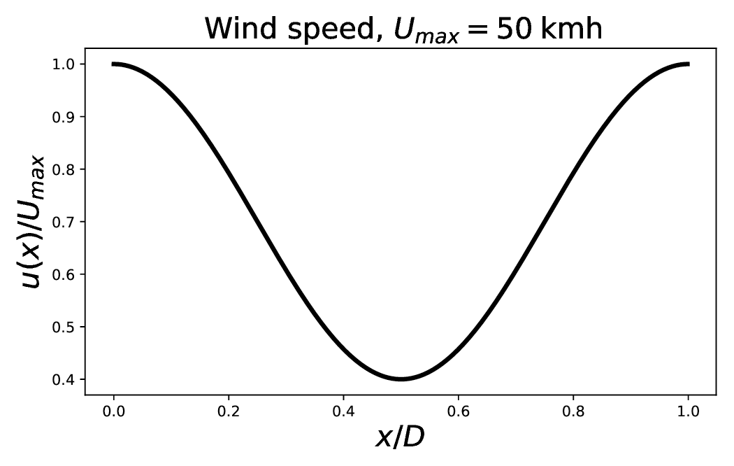
Figure 1 Pre-defined heterogeneous and stationary wind field u(x) used for the transport simulations.

For this experiment, the mean state 𝒳, the variance field V, and the aspect-tensor field s are initialized homogeneously with values 𝒳⁰=1 and V⁰=(σ⁰)², where σ⁰=0.1, and $s^{\mathrm{0}}=(l_{\mathrm{h}}^{\mathrm{0}}{)}^{\mathrm{2}}$, where $l_{\mathrm{h}}^{\mathrm{0}}=\mathrm{15}\mathrm{\Delta }x\simeq \mathrm{62.2}$ km. This initial setting also corresponds to the initial state of the PKF dynamics in Eq. (10). With regards to the domain chosen, this setting for the length scale is in agreement with practical estimations often encountered (Ménard et al., 2016). The wind field considered, shown in Fig. 1, is defined by $u\left(x\right)=(\mathrm{35}+\mathrm{15}\cos (\mathrm{2}\mathit{\pi }x\left)\right)/D$ and modellizes a wind of average intensity 35 km h⁻¹ and of maximum speed $U_{max}=\mathrm{50}$ km h⁻¹. The characteristic time τ_adv is defined by ${\mathit{\tau }}_{\mathrm{adv}}=D/\stackrel{\mathrm{‾}}{u}\simeq \mathrm{28.5}$ h and approximately corresponds to the time of a revolution of the tracer around the periodic domain. The simulation time horizon T=t_end is set to t_end=3τ_adv.

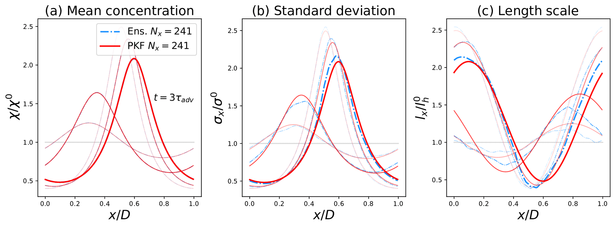
Figure 2 Comparison of the (low-resolution) forecasts (N_x=241) of the mean state (a), the forecast-error standard deviation $\mathit{\sigma }=\sqrt{V}$ (b) and the forecast-error length scale $l=\mathrm{1}/\sqrt{g}=\sqrt{s}$ (c), shown at times $t=[\mathrm{0.6},\mathrm{1.2},\mathrm{1.8},\mathrm{2.4},\mathrm{3.0}]{\mathit{\tau }}_{\mathrm{adv}}$, computed from the PKF (red lines) and compared with the diagnoses of an ensemble of N_e=6400 forecasts (cyan dash-dotted lines). The more transparent the curve, the closer it is to t=0. The horizontal grey lines represent the initial conditions.

The dynamics of the uncertainty show in Fig. 2 that the tracer tends to concentrate in the deceleration zones (see Fig. 1 from x=0 to x=0.5) and to dilute in the acceleration zones (from x=0.5 to x=1.0) (Fig. 2a). This observation also applies to the standard-deviation field in Fig. 2b, as it is governed by the same dynamics as the tracer's concentration (it is straightforward to calculate the dynamics of σ using the dynamics of the variance in Eq. 10b). In Fig. 2c, the length scales (1D equivalent of the anisotropy) are subject to two processes: a pure transport term (left-hand side of Eq. 10c) and a production term related to the wind sheer (right-hand side of Eq. 10c). This production term is positive (negative) when the wind field is accelerating (decelerating), indicating an increase (decrease) in the length scales in the accelerating (decelerating) wind regions. In contrast to the concentrations and standard-deviation fields (governed by a conservative transport), the average value of the length scales varies in time; however, numerical experiments (not shown here) have shown that it oscillates around the initial value.

Regarding the performances of the two methods, the PKF forecast results for the error statistics are quite similar to the one diagnosed from the ensemble, i.e. the EnKF for this test bed. The forecasts of the concentrations in Fig. 2a are identical for both methods. Although the dynamics for the variance in Eq. (10b) and the anisotropy in Eq. (10c) are exact in the PKF system, a significant difference is observed between the forecasts of the two methods (Fig. 2b and c). This difference is due to errors in the EnKF rather than errors in the PKF. Note that the model error that affects the EnKF can be corrected by performing high-resolution simulations (N_x=723; see Appendix A for details). This highlights some of the limitations of the numerical validation of the PKF by an ensemble method in the presence of model error. This numerical experiment shows that the PKF is able to produce high-quality forecasts of the diagnoses of the forecast-error statistics, a result that is confirmed by looking at the forecast-error correlation functions (see Appendix B).

This example shows the motivation behind the PKF: it is able to predict the (main parameters of the) error covariance with a good skill and at a low numerical cost. This low numerical cost first concerns the computer memory: the information contained in a covariance matrix of size $\mathcal{O}\left(N_x^{\mathrm{2}}\right)$ in the ensemble case is reduced by the covariance model in Eq. (7), which only needs a few parameters of sizes of order 𝒪(N_x) (with 𝒪 being the “Big O” notation, meaning “proportional to”). However, the low numerical cost also concerns the time taken to predict the uncertainty: the PKF only relies on the single time integration of Eq. (10), which represents the cost of 3 time integrations of the initial dynamics in Eq. (9b) compared to the 6400 time integrations required for the ensemble used here.

As another advantage, the PKF provides information about the physics of the uncertainty: when ensemble diagnosis only observes the time evolution of the statistics without any explications, the PKF provides a simplified proxy that details the origins of these statistical evolutions with only three equations, and thus the PKF improves our knowledge of uncertainty dynamics.

3 Toward a multivariate formulation of the PKF

The exploration of the multivariate extension is now addressed. For multivariate problems, a modellization of the cross-correlation functions (or inter-species correlation functions) is needed. Moreover, it would be convenient to introduce a multivariate covariance model that extends the univariate VLATcov model, as the heterogeneous Gaussian model (Eq. 7), to take advantage of the PKF dynamics of univariate statistics.

Because multivariate modelling is a difficult topic, a multivariate covariance model is proposed in a simplified test bed in Sect. 3.1, where data-driven modelling is considered to determine a multivariate covariance model and its parameters. Next, the multivariate PKF is formulated, detailing the prediction and the analysis steps in Sect. 3.2. Finally, two numerical assimilation experiments are conducted in Sect. 3.3.

3.1 Development of a proxy multivariate covariance model

3.1.1 Introduction of the simplified chemical transport model

To explore a multivariate formulation of the PKF, a simplified chemical transport model is introduced that mimics the MOCAGE framework. This simplified CTM contains the essential features of what can be found in a more realistic CTM, i.e. advection, multiple chemical species, and non-linearities.

To do so, a 1D periodic domain of coordinate x is considered, where two non-linearly reactive chemical species, A(t,x) and B(t,x), are advected in a conservative way by a heterogeneous and stationary wind field u(x). The non-linear reaction is given by the Lotka–Volterra (LV) equations (see Appendix C), which leads to the coupled dynamics

$$\begin{array}{}\text{(13a)}& {\displaystyle }& {\displaystyle }{\partial }_{t}A+u{\partial }_{x}A=-A{\partial }_{x}u+k_{\mathrm{1}}A-k_{\mathrm{2}}AB,\text{(13b)}& {\displaystyle }& {\displaystyle }{\partial }_{t}B+u{\partial }_{x}B=-B{\partial }_{x}u+k_{\mathrm{2}}AB-k_{\mathrm{3}}B,\end{array}$$

where the transport is written following the univariate 1D example in Eq. (9b) and where the LV reaction appears as the last two terms on the right-hand side of each prognostic equation. The constants k₁, k₂, and k₃ characterize the reaction rates: k₁ corresponds to the rate at which A is produced, constant k₂ represents the rate at which the chemical reactions between A and B produce 2B, and k₃ describes the decay rate for species B. Note that, at a formal level, the state vector associated with Eq. (13) is then $\mathcal{X}(t,x)=(A,B)(t,x)$.

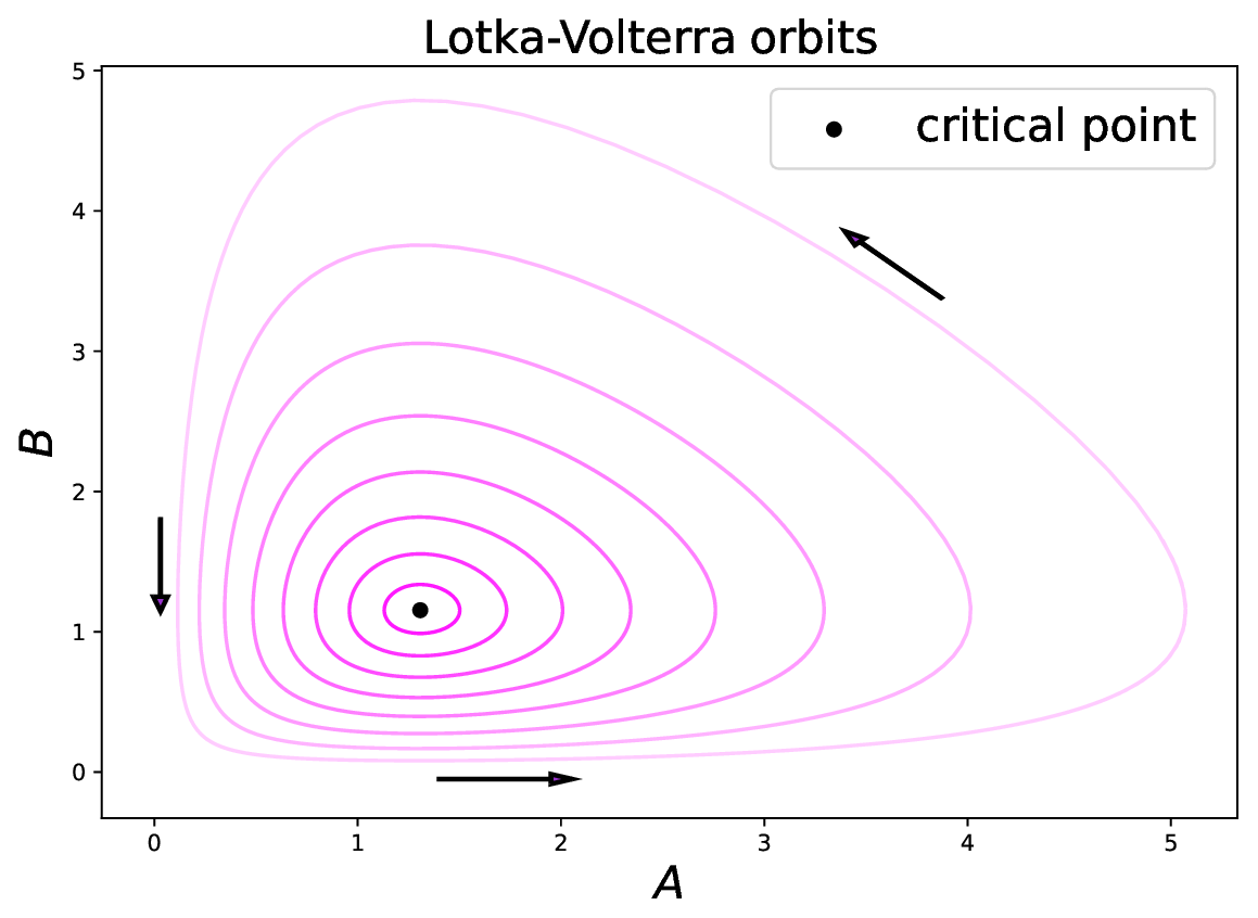
Figure 3 Numerical simulations of the Lotka–Volterra dynamical system whose solutions are periodical orbits (purple curves with different transparencies), flowing anti-clockwise around the critical point $(A_{\mathrm{c}},B_{\mathrm{c}})=\left(\frac{k_{\mathrm{3}}}{k_{\mathrm{1}}},\frac{k_{\mathrm{1}}}{k_{\mathrm{2}}}\right)$ (black dot).

Considered as a dynamical system of ordinary equations and represented in the phase space (A,B), the solutions of the Lotka–Volterra dynamics are periodical orbits flowing around the critical point of coordinates $(A_{\mathrm{c}},B_{\mathrm{c}})=\left(\frac{k_{\mathrm{3}}}{k_{\mathrm{1}}},\frac{k_{\mathrm{1}}}{k_{\mathrm{2}}}\right)$, as shown in Fig. 3. This is the kind of time evolution observed at each grid point when there is no wind (u=0).

In this multivariate framework, the error-covariance matrix P=𝔼(ε_𝒳(ε_𝒳)^T) associated with the state $\mathcal{X}=(A,B)$, of error ${\mathit{\epsilon }}_{\mathcal{X}}=({\mathit{\epsilon }}_A,{\mathit{\epsilon }}_B)$, reads as a block matrix

$$\begin{array}{}\text{(14)}& \mathbf{P}=\left(\begin{array}{cc}{\mathbf{P}}_A& {\left({\mathbf{P}}_{AB}\right)}^{\mathrm{T}}\\ {\mathbf{P}}_{AB}& {\mathbf{P}}_B\end{array}\right),\end{array}$$

where P_A and P_B are the auto-covariance matrices of the errors, and P_AB is the cross-covariance matrix, or the inter-species covariance matrix, of the errors. Note that, in general, P_AB is not symmetric, i.e. ${\left({\mathbf{P}}_{AB}\right)}^{\mathrm{T}}\ne {\mathbf{P}}_{AB}$. The two-point cross-covariance function ${\mathbf{P}}_{AB}(x,y)=\stackrel{\mathrm{‾}}{{\mathit{\epsilon }}_A\left(x\right){\mathit{\epsilon }}_B\left(y\right)}$ between grid points of coordinates x and y is written as

$$\begin{array}{}\text{(15)}& {\mathbf{P}}_{AB}(x,y)=\sqrt{V_A\left(x\right)}\sqrt{V_B\left(y\right)}{\mathit{\rho }}_{AB}(x,y),\end{array}$$

where

$$\begin{array}{}\text{(16)}& {\mathit{\rho }}_{AB}(x,y)={\displaystyle \frac{{\mathbf{P}}_{AB}(x,y)}{\sqrt{V_A\left(x\right)}\sqrt{V_B\left(y\right)}}}\end{array}$$

is the cross-correlation function. The cross-correlation function is not symmetric in general, i.e. ${\mathit{\rho }}_{AB}(x,y)\ne {\mathit{\rho }}_{AB}(y,x)$. In particular, if C_AB denotes the associated cross-correlation matrix, then ${\mathbf{C}}_{AB}\ne {\left({\mathbf{C}}_{AB}\right)}^{\mathrm{T}}$.

From a covariance-modelling point of view, and from the perspective of the PKF, the univariate covariances P_A and P_B could be approximated by a VLATcov model, e.g. P(V_A,s_A). Moreover, the single-point cross-covariance field defined as $V_{AB}\left(x\right)=\stackrel{\mathrm{‾}}{{\mathit{\epsilon }}_A\left(x\right){\mathit{\epsilon }}_B\left(x\right)}$ will appear in the dynamics of V_A and V_B because of the coupling due to LV equations and should be considered a natural parameter for a multivariate PKF. At this stage, the question is whether it is possible to approximate the two-point cross-covariance functions P_AB(x,y) knowing the parameters $(\stackrel{\mathrm{‾}}{A},\stackrel{\mathrm{‾}}{B},V_A,V_B,V_{AB},s_A,s_B)$, which are functions of x.

Since no multivariate modelling extending the VLATcov model is available, a numerical exploration of the dynamics of multivariate statistics is performed for the LV CTM so as to guess a proxy for the cross-covariance functions.

3.1.2 Ensemble of multivariate forecasts

Compared to the univariate experiment described in Sect. 2.4, without a multivariate covariance model, it is not possible to sample a multivariate ensemble. For this reason, the errors for the two chemical species are assumed to be decorrelated at the initial time t=0, so that the error-covariance matrix, P⁰, is the block diagonal

$$\begin{array}{}\text{(17)}& {\mathbf{P}}^{\mathrm{0}}=\left(\begin{array}{cc}{\mathbf{P}}_A^{\mathrm{0}}& \mathrm{0}\\ \mathrm{0}& {\mathbf{P}}_B^{\mathrm{0}}\end{array}\right),\end{array}$$

where ${\mathbf{P}}_A^{\mathrm{0}}$ $\left({\mathbf{P}}_B^{\mathrm{0}}\right)$ is the univariate covariance associated with error in A (B). Following the ensemble generation of Sect. 2.4, the univariate covariance matrices are chosen as the two VLATcov matrices ${\mathbf{P}}_A^{\mathrm{0}}=\mathbf{P}(V_A^{\mathrm{0}},s_A^{\mathrm{0}})$ and ${\mathbf{P}}_B^{\mathrm{0}}=\mathbf{P}(V_B^{\mathrm{0}},s_B^{\mathrm{0}})$. Then, an ensemble of N_e=6400 initial conditions $({\mathcal{X}}_k^{\mathrm{0}}{)}_{k\in [\mathrm{1},N_{\mathrm{e}}]}$ is sampled, with, for each k, ${\mathcal{X}}_k^{\mathrm{0}}={\mathcal{X}}^{\mathrm{0}}+{\left({\mathbf{P}}^{\mathrm{0}}\right)}^{\mathrm{1}/\mathrm{2}}{\mathit{\zeta }}_k$, where ${\mathcal{X}}^{\mathrm{0}}=(A^{\mathrm{0}},B^{\mathrm{0}})$ and ${\left({\mathbf{P}}^{\mathrm{0}}\right)}^{\mathrm{1}/\mathrm{2}}$ are the block-diagonal matrix ${\left({\mathbf{P}}^{\mathrm{0}}\right)}^{\mathrm{1}/\mathrm{2}}=\mathrm{diag}\left(\mathbf{P}(V_A^{\mathrm{0}},s_A^{\mathrm{0}}{)}^{\mathrm{1}/\mathrm{2}},\mathbf{P}(V_B^{\mathrm{0}},s_B^{\mathrm{0}}{)}^{\mathrm{1}/\mathrm{2}}\right)$. This time, ζ_k is a sample of 𝒩(0,I_n) with n=2N_x. The domain is discretized into N_x=723 grid points.

For the simulation, the fields A⁰ and B⁰ are set to the constants A⁰=1.2 and B⁰=0.8. The univariate parameters are set to ${\mathit{\sigma }}_A^{\mathrm{0}}=\mathrm{0.1}\cdot A^{\mathrm{0}}$, ${\mathit{\sigma }}_B^{\mathrm{0}}=\mathrm{0.1}\cdot B^{\mathrm{0}}$, and $s_A^{\mathrm{0}}=s_A^{\mathrm{0}}=l_{\mathrm{h}}^{\mathrm{2}}$ with $l_{\mathrm{h}}=\mathrm{45}\mathrm{\Delta }x\simeq \mathrm{62}$ km. The reaction rates of LV are set to $(k_{\mathrm{1}},k_{\mathrm{2}},k_{\mathrm{3}})=(\mathrm{0.075},\mathrm{0.065},\mathrm{0.085})$. The time integration follows the numerical setting used for the univariate simulation presented in Sect. 2.4 and leads to an ensemble of N_e=6400 multivariate forecasts.

While there is no cross-correlation at the initial condition, the coupling provided by the LV equations should introduce a non-zero cross-correlation between errors in A and B, and this can be diagnosed from the computation of the ensemble estimation of the two-point forecast-error cross-covariance function P_AB(x,y) at time t, given by

$$\begin{array}{}\text{(18)}& {\widehat{\mathbf{P}}}_{AB}(t,x,y)={\displaystyle \frac{\mathrm{1}}{N_{\mathrm{e}}-\mathrm{1}}}\sum _{k=\mathrm{1}}^{N_{\mathrm{e}}}{\mathit{\epsilon }}_{A,k}(t,x){\mathit{\epsilon }}_{B,k}(t,y),\end{array}$$

with ${\mathit{\epsilon }}_{A,k}(t,x)=A_k(t,x)-\widehat{A}(t,x)$ and ${\mathit{\epsilon }}_{B,k}(t,y)=B_k(t,y)-\widehat{B}(t,y)$, where $\widehat{A}$ and $\widehat{B}$ are the empirical means of the ensemble of forecasts (A_k) and (B_k), from which an estimation of the cross-correlation functions ${\widehat{\mathit{\rho }}}_{AB}(t,x,y)$ and matrix ${\widehat{\mathbf{C}}}_{AB}\left(t\right)$ can be deduced.

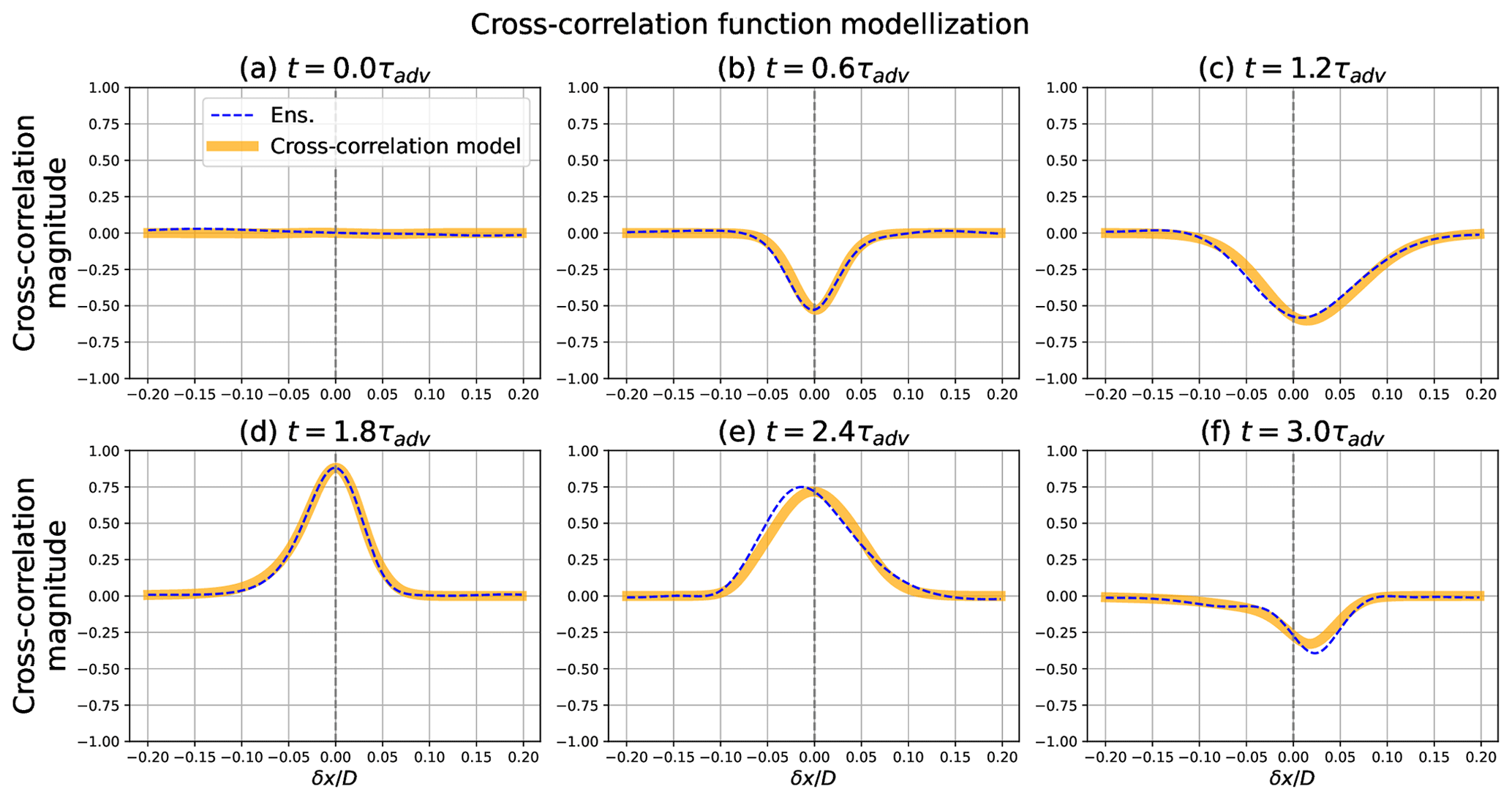
Figure 4 Evaluation of the cross-correlation model $r_{AB}(x_L,\cdot )$ (bold orange line) versus the ensemble estimation of the cross-correlation ${\mathit{\rho }}_{AB}(x_L,\cdot )$ (blue dashed line) with respect to the location x_l=0.5 and times $t=[\mathrm{0.0},\mathrm{0.6},\mathrm{1.2},\mathrm{1.8},\mathrm{2.4},\mathrm{3.0}]{\mathit{\tau }}_{\mathrm{adv}}$.

Figure 4 shows the time evolution of the cross-correlation with respect to the grid point x_l=0.5, i.e. the function ${\mathit{\rho }}_{AB}(x_{\mathrm{l}},\cdot )$. As has been specified, the cross-correlation is zero at t=0 (Fig. 4a). Then, as expected, the cross-correlation evolves along the time, presenting an anti-cross-correlation at t=0.6τ_adv (Fig. 4b) and then a positive one at t=1.8τ_adv (Fig. 4d). At t=2.4τ_adv (Fig. 4e), the cross-correlation appears clearly asymmetric while reaching its maximum value at a y strictly lower than x_l.

3.1.3 Formulation of a proxy for the cross-correlation

Now, a proxy for the cross-correlation is introduced from the data set of multivariate forecasts.

After a trial-and-error process, and inspired by the VLATcov model in Eq. (7), the following expression,

$$\begin{array}{}\text{(19)}& \begin{array}{rl}{r}_{AB}(\mathit{x},\mathit{y})& ={\displaystyle \frac{\mathrm{1}}{\mathrm{2}}}\left({\displaystyle \frac{V_{AB}\left(\mathit{x}\right)}{{\mathit{\sigma }}_A\left(\mathit{x}\right){\mathit{\sigma }}_B\left(\mathit{x}\right)}}+{\displaystyle \frac{V_{AB}\left(\mathit{y}\right)}{{\mathit{\sigma }}_A\left(\mathit{y}\right){\mathit{\sigma }}_B\left(\mathit{y}\right)}}\right)\\ & \exp \left(-\left|\right|\mathit{x}-\mathit{y}|{|}_{\left[\frac{\mathrm{1}}{\mathrm{4}}\right(s_A\left(\mathit{x}\right)+s_B\left(\mathit{x}\right)+s_A\left(\mathit{y}\right)+s_B\left(\mathit{y}\right)){]}^{-\mathrm{1}}}^{\mathrm{2}}\right),\end{array}\end{array}$$

as a function of the known parameters $\mathcal{P}=(V_A,V_B,V_{AB},s_A,s_B)$, has been proposed as a proxy for the cross-correlation ρ_AB, i.e. $r_{AB}(x,y)\approx {\mathit{\rho }}_{AB}(x,y)$. It consists of an interpolation by the mean of the cross-correlation values at location x and y, multiplied by a Gaussian kernel, where the univariate aspect tensor has been substituted by the mean of the aspect tensors of all chemical species. The resulting proxy for the cross-correlation matrix is denoted by ${\mathbf{C}}_{AB}^{\mathrm{proxy}}\left(\mathcal{P}\right)$.

One of the main advantages of considering a simple analytic formula is that it can be extended to a problem with more chemical species and for a domain of a higher dimension.

Note that formulation Eq. (19) is symmetric ($r_{AB}(x,y)=r_{AB}(y,x)$), while cross-correlations are not symmetric in general (${\mathit{\rho }}_{AB}(x,y)\ne {\mathit{\rho }}_{AB}(y,x)$), but this expression leverages all the parameters known at locations x and y. However, the function $r_{AB,x}\left(\mathit{\delta }x\right)=r_{AB}(x,x+\mathit{\delta }x)$ is not necessarily symmetric in δx, where, in general, $r_{AB,x}\left(\mathit{\delta }x\right)\ne r_{AB,x}(-\mathit{\delta }x)$.

To assess the skill of the proxy, Fig. 4 shows the functions $r_{AB}(x_{\mathrm{l}},\cdot )$ (computed from Eq. 19 with the ensemble-estimated parameters $\widehat{\mathcal{P}}\left(t\right)=(\widehat{V_A},\widehat{V_B},\widehat{V_{AB}},\widehat{s_A},\widehat{s_B})\left(t\right)$) compared with the ensemble-estimated cross-correlation ${\mathit{\rho }}_{AB}(x_{\mathrm{l}},\cdot )$. At a qualitative level, the functions r_AB are in accordance with the cross-correlation ρ_AB of reference for all the panels. Note that, while r_AB is symmetric, the functions $r_{AB}(x_{\mathrm{l}},\cdot )$ can be asymmetric as they appear in Fig. 4c and f.

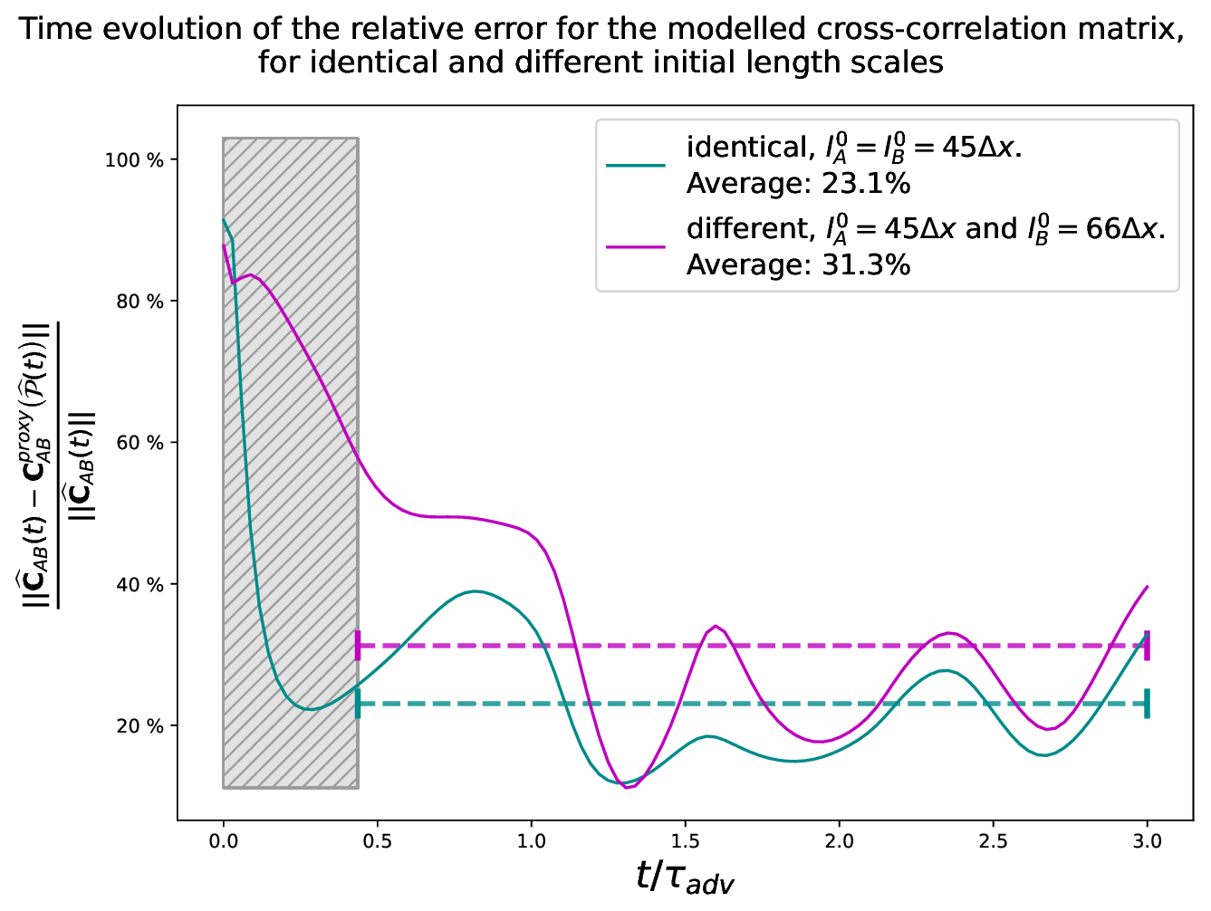
Figure 5 Time evolutions of the relative errors between the empirical cross-correlation matrix (EnKF) and the proxy-generated cross-correlation matrix fitted with EnKF-diagnosed parameters for two different settings of the initial length scales: equal length scales with $l_A^{\mathrm{0}}=l_B^{\mathrm{0}}=\mathrm{45}\mathrm{\Delta }x\approx \mathrm{66}$ km (turquoise line) and different length scales with $l_A^{\mathrm{0}}=\mathrm{45}\mathrm{\Delta }x$ and $l_B^{\mathrm{0}}=\mathrm{66}\mathrm{\Delta }x\approx \mathrm{91}$ km (mauve line). The results being dominated by sampling noise for t<0.45, they are not retained (grey hatching) for the computation of the temporal averages (dashed segments).

At a quantitative level, Fig. 5 shows the time evolution of the relative error $\frac{\left|\right|{\widehat{\mathbf{C}}}_{AB}\left(t\right)-{\mathbf{C}}_{AB}^{\mathrm{proxy}}\left(\widehat{\mathcal{P}}\right(t\left)\right)\left|\right|}{\left|\right|{\widehat{\mathbf{C}}}_{AB}\left(t\right)\left|\right|}$, where $\left|\right|\mathbf{U}\left|\right|=\sqrt{\mathrm{Tr}\left({\mathbf{UU}}^{\mathrm{T}}\right)}$ is the Frobenius matrix norm where Tr is the trace operator, ${\widehat{\mathbf{C}}}_{AB}\left(t\right)$ is the ensemble estimation of the cross-correlation matrix, and ${\mathbf{C}}_{AB}^{\mathrm{proxy}}\left(\widehat{\mathcal{P}}\right(t\left)\right)$ is the proxy for the cross-correlation matrix fitted with ensemble-estimated parameters $\widehat{\mathcal{P}}\left(t\right)$. Two different experiments are shown depending on whether the initial length scales for A and B are equal, $l_A^{\mathrm{0}}=l_B^{\mathrm{0}}=\mathrm{45}\mathrm{\Delta }x\approx \mathrm{66}$ km (turquoise lines), or different, $l_A^{\mathrm{0}}\approx \mathrm{66}$ km, but $l_B^{\mathrm{0}}=\mathrm{66}\mathrm{\Delta }x\approx \mathrm{91}$ km (purple lines).

As the two multivariate error fields are uncorrelated at the initial time, the true cross-correlation matrix C_AB(t=0) is zero. However, the ensemble used in the estimation of ${\widehat{\mathbf{C}}}_{AB}(t=\mathrm{0})$ being finite, this produces a spurious non-zero cross-correlation leading to a non-zero matrix and to a relative error larger than 80 %. Then, the first instants of the simulation are dominated by the sampling noise, and they are excluded for the analysis of the results (grey hatching). After t≃0.45, the experiments offer valid results and lead to temporal averages of 23.1 % when $l_A^{\mathrm{0}}=l_B^{\mathrm{0}}$ (turquoise dashed line) and 31.3 % when $l_A^{\mathrm{0}}\ne l_B^{\mathrm{0}}$. Note that the effect of the sampling noise can lead to an overestimation of 8 % for this kind of experiment (Pannekoucke, 2021a).

According to our knowledge, no proxy of cross-correlations similar to Eq. (19) has been introduced up to now as a possible proxy of cross-correlations. As mentioned above, r_AB does not share the same property of the cross-correlation (e.g. r_AB is symmetric, while ρ_AB is not), and thus there is no guarantee that a multivariate covariance model based on the proxy r_AB will lead to a true covariance matrix: such a multivariate covariance model is symmetric because r_AB is symmetric but not necessarily positive definite, although it may not be essential for the PKF applications.

Despite the limitations of the proxy, a multivariate extension of the univariate VLATcov model is explored below, where the cross-correlation is approximated by the proxy in Eq. (19). This leads to a multivariate VLATcov model of parameters for fields $(V_{AB},V_A,V_B,s_A,s_B)$, for which we can formulate a PKF.

3.2 Formulation and simplification of the parameter dynamics and analysis

3.2.1 PKF dynamics for the LV CTM

The computation of the PKF dynamics leverages the SymPKF package which, applied to the dynamics Eq. (13), provides the following system of coupled equations.

$$\begin{array}{}\text{(20a)}& {\displaystyle }{\partial }_{t}A+u{\partial }_{x}A=-A{\partial }_{x}u+k_{\mathrm{1}}A-k_{\mathrm{2}}AB-k_{\mathrm{2}}{V}_{AB}\text{(20b)}& {\displaystyle }{\partial }_{t}B+u{\partial }_{x}B=-B{\partial }_{x}u-k_{\mathrm{3}}B+k_{\mathrm{2}}AB+k_{\mathrm{2}}{V}_{AB}\text{(20c)}& {\displaystyle }\begin{array}{rl}& {\partial }_t{V}_{AB}+u{\partial }_x{V}_{AB}=-\mathrm{2}{V}_{AB}{\partial }_{x}u\\ & +V_{AB}(k_{\mathrm{1}}-k_{\mathrm{2}}B-k_{\mathrm{3}}+k_{\mathrm{2}}A)+k_{\mathrm{2}}{V}_{A}B-k_{\mathrm{2}}{V}_{B}A\end{array}\text{(20d)}& {\displaystyle }\begin{array}{rl}& {\partial }_t{V}_A+u{\partial }_x{V}_A=-\mathrm{2}{V}_A{\partial }_{x}u\\ & +\mathrm{2}\left[V_A\right(k_{\mathrm{1}}-k_{\mathrm{2}}B)-k_{\mathrm{2}}A{V}_{AB}]\end{array}\text{(20e)}& {\displaystyle }\begin{array}{rl}& {\partial }_t{V}_B+u{\partial }_x{V}_B=-\mathrm{2}{V}_B{\partial }_{x}u\\ & +\mathrm{2}\left[V_B\right(-k_{\mathrm{3}}+k_{\mathrm{2}}A)+k_{\mathrm{2}}B{V}_{AB}]\end{array}\text{(20f)}& {\displaystyle }\begin{array}{rl}& {\partial }_t{s}_A+\underset{T_{A,\text{adv-}\mathrm{1}}}{\underbrace{u{\partial }_x{s}_A}}=\underset{T_{A,\text{adv-}\mathrm{2}}}{\underbrace{\mathrm{2}{s}_A{\partial }_{x}u}}-\underset{T_{A,\text{chem-}\mathrm{1}}}{\underbrace{{\displaystyle \frac{\mathrm{2}{k}_{\mathrm{2}}A{V}_{AB}{s}_A}{V_A}}}}\\ & +\underset{T_{A,\text{chem-}\mathrm{2}}}{\underbrace{{\displaystyle \frac{\mathrm{2}{k}_{\mathrm{2}}A{\mathit{\sigma }}_B{s}_A^{\mathrm{2}}\stackrel{\mathrm{‾}}{{\partial }_x{\stackrel{\mathrm{̃}}{\mathit{\epsilon }}}_A{\partial }_x{\stackrel{\mathrm{̃}}{\mathit{\epsilon }}}_B}}{{\mathit{\sigma }}_A}}}}+\underset{T_{A,\text{chem-}\mathrm{3}}}{\underbrace{{\displaystyle \frac{k_{\mathrm{2}}A{s}_A^{\mathrm{2}}\stackrel{\mathrm{‾}}{{\stackrel{\mathrm{̃}}{\mathit{\epsilon }}}_B{\partial }_x{\stackrel{\mathrm{̃}}{\mathit{\epsilon }}}_a}{\partial }_x{V}_B}{{\mathit{\sigma }}_A{\mathit{\sigma }}_B}}}}\\ & -\underset{T_{A,\text{chem-}\mathrm{4}}}{\underbrace{{\displaystyle \frac{k_{\mathrm{2}}A{\mathit{\sigma }}_B{s}_A^{\mathrm{2}}\stackrel{\mathrm{‾}}{{\stackrel{\mathrm{̃}}{\mathit{\epsilon }}}_B{\partial }_x{\stackrel{\mathrm{̃}}{\mathit{\epsilon }}}_A}{\partial }_x{V}_B}{V_A^{\frac{\mathrm{3}}{\mathrm{2}}}}}}}+\underset{T_{A,\text{chem-}\mathrm{5}}}{\underbrace{{\displaystyle \frac{\mathrm{2}{k}_{\mathrm{2}}{\mathit{\sigma }}_B{s}_A^{\mathrm{2}}\stackrel{\mathrm{‾}}{{\stackrel{\mathrm{̃}}{\mathit{\epsilon }}}_B{\partial }_x{\stackrel{\mathrm{̃}}{\mathit{\epsilon }}}_A}{\partial }_{x}A}{{\mathit{\sigma }}_A}}}}\end{array}\text{(20g)}& {\displaystyle }\begin{array}{rl}& {\partial }_t{s}_B+\underset{T_{B,\text{adv-}\mathrm{1}}}{\underbrace{u{\partial }_x{s}_B}}=\underset{T_{B,\text{adv-}\mathrm{2}}}{\underbrace{\mathrm{2}{s}_B{\partial }_{x}u}}+\underset{T_{B,\text{chem-}\mathrm{1}}}{\underbrace{{\displaystyle \frac{\mathrm{2}{k}_{\mathrm{2}}B{V}_{AB}{s}_B}{V_B}}}}\\ & -\underset{T_{B,\text{chem-}\mathrm{2}}}{\underbrace{{\displaystyle \frac{\mathrm{2}{k}_{\mathrm{2}}B{\mathit{\sigma }}_A{s}_B^{\mathrm{2}}\stackrel{\mathrm{‾}}{{\partial }_x{\stackrel{\mathrm{̃}}{\mathit{\epsilon }}}_A{\partial }_x{\stackrel{\mathrm{̃}}{\mathit{\epsilon }}}_B}}{{\mathit{\sigma }}_B}}}}-\underset{T_{B,\mathrm{chem}-\mathrm{3}}}{\underbrace{{\displaystyle \frac{k_{\mathrm{2}}B{s}_B^{\mathrm{2}}\stackrel{\mathrm{‾}}{{\stackrel{\mathrm{̃}}{\mathit{\epsilon }}}_A{\partial }_x{\stackrel{\mathrm{̃}}{\mathit{\epsilon }}}_B}{\partial }_x{V}_A}{{\mathit{\sigma }}_A{\mathit{\sigma }}_B}}}}\\ & +\underset{T_{B,\text{chem-}\mathrm{4}}}{\underbrace{{\displaystyle \frac{k_{\mathrm{2}}B{\mathit{\sigma }}_A{s}_B^{\mathrm{2}}\stackrel{\mathrm{‾}}{{\stackrel{\mathrm{̃}}{\mathit{\epsilon }}}_A{\partial }_x{\stackrel{\mathrm{̃}}{\mathit{\epsilon }}}_B}{\partial }_x{V}_B}{V_B^{\frac{\mathrm{3}}{\mathrm{2}}}}}}}-\underset{T_{B,\text{chem-}\mathrm{5}}}{\underbrace{{\displaystyle \frac{\mathrm{2}{k}_{\mathrm{2}}{s}_B^{\mathrm{2}}\stackrel{\mathrm{‾}}{{\stackrel{\mathrm{̃}}{\mathit{\epsilon }}}_A{\partial }_x{\stackrel{\mathrm{̃}}{\mathit{\epsilon }}}_B}{\partial }_{x}B}{{\mathit{\sigma }}_B}}}}\end{array}\end{array}$$

The overlines of the mean states $\stackrel{\mathrm{‾}}{A}$ and $\stackrel{\mathrm{‾}}{B}$ have been discarded for the sake of simplicity. The PKF is a second-order filter in which the variances of the fluctuations modify the time evolution of the mean states, e.g. by the term −k₂V_AB of Eq. (20a).

For the dynamics of the anisotropy in Eqs. (20f) and (20g), the contributions due to the transport (to the chemistry) are labelled $T_{(\cdot ),\text{adv-}(\cdot )}$ ($T_{(\cdot ),\text{chem-}(\cdot )}$) for identification.

Note that the dynamics induced by the transport process are exact, as mentioned in Sect. 2.4. In the PKF system in Eq. (20), the dynamics of the mean concentrations A and B, variances V_A and V_B, and cross-covariance V_AB, Eqs. (20a) to (20e), are independent of the anisotropy field in Eqs. (20f) and (20g). The reciprocal is not true: the anisotropy field dynamics (Eqs. 20f–20g) are forced by the means, the variances, the cross-covariances, and their spatial heterogeneity. Equations (20a) and 20b also indicate an interaction between the cross-covariance and the mean concentrations.

The dynamics of the aspect tensors, Eqs. (20f) and (20g), are not closed: some terms are expressed as expectations of the normalized errors ${\stackrel{\mathrm{̃}}{\mathit{\epsilon }}}_A={\mathit{\epsilon }}_A/\sqrt{V_A}$ and ${\stackrel{\mathrm{̃}}{\mathit{\epsilon }}}_B={\mathit{\epsilon }}_B/\sqrt{V_B}$. These open terms cannot be directly expressed using the available parameters, preventing the forecast of the error statistics.

3.2.2 Closure of the PKF dynamics

A closure is proposed for the LV CTM multivariate PKF dynamics. Note that the open terms of the PKF dynamics Eq. (20) can be related to spatial derivatives of the cross-correlation Eq. (16), e.g. $\stackrel{\mathrm{‾}}{{\stackrel{\mathrm{̃}}{\mathit{\epsilon }}}_A{\partial }_x{\stackrel{\mathrm{̃}}{\mathit{\epsilon }}}_B}\left(x\right)=\left({\partial }_x{\mathit{\rho }}_{AB}\right)(x,x)$ or $\stackrel{\mathrm{‾}}{{\partial }_x{\stackrel{\mathrm{̃}}{\mathit{\epsilon }}}_A{\partial }_x{\stackrel{\mathrm{̃}}{\mathit{\epsilon }}}_B}\left(x\right)=\left({\partial }_{xy}{\mathit{\rho }}_{AB}\right)(x,x)$, leading to a closure of the PKF dynamics when the proxy r_AB Eq. (19) is used in place of the true cross-correlation ρ_AB. However, numerical investigation of this closure did not lead to good results (not shown here).

From a detailed quantification of the impact of the chemistry alone (see Appendix D1) and of the relative contributions comparing the importance of the advection versus the chemistry (see Appendix D2), the result is that the advection contributes 80 % of the anisotropy dynamics, while 20 % are due to the chemistry. Since the advection mainly leads the dynamics of the anisotropy, this suggests that the contribution of the chemistry in Eqs. (20f) and (20g) be removed, which leads to a closure of the PKF dynamics in Eq. (20) as

$$\begin{array}{}\text{(21a)}& {\displaystyle }{\partial }_{t}A+u{\partial }_{x}A=-A{\partial }_{x}u+k_{\mathrm{1}}A-k_{\mathrm{2}}AB-k_{\mathrm{2}}{V}_{AB},\text{(21b)}& {\displaystyle }{\partial }_{t}B+u{\partial }_{x}B=-B{\partial }_{x}u-k_{\mathrm{3}}B+k_{\mathrm{2}}AB+k_{\mathrm{2}}{V}_{AB},\text{(21c)}& {\displaystyle }\begin{array}{rl}& {\partial }_t{V}_{AB}+u{\partial }_x{V}_{AB}=-\mathrm{2}{V}_{AB}{\partial }_{x}u\\ & +V_{AB}(k_{\mathrm{1}}-k_{\mathrm{2}}B-k_{\mathrm{3}}+k_{\mathrm{2}}A)+k_{\mathrm{2}}{V}_{A}B-k_{\mathrm{2}}{V}_{B}A,\end{array}\text{(21d)}& {\displaystyle }\begin{array}{rl}& {\partial }_t{V}_A+u{\partial }_x{V}_A=-\mathrm{2}{V}_A{\partial }_{x}u\\ & +\mathrm{2}\left[V_A\right(k_{\mathrm{1}}-k_{\mathrm{2}}B)-k_{\mathrm{2}}A{V}_{AB}],\end{array}\text{(21e)}& {\displaystyle }\begin{array}{rl}& {\partial }_t{V}_B+u{\partial }_x{V}_B=-\mathrm{2}{V}_B{\partial }_{x}u\\ & +\mathrm{2}\left[V_B\right(-k_{\mathrm{3}}+k_{\mathrm{2}}A)+k_{\mathrm{2}}B{V}_{AB}],\end{array}\text{(21f)}& {\displaystyle }{\partial }_t{s}_A=-u{\partial }_x{s}_A+\mathrm{2}{s}_A{\partial }_{x}u,\text{(21g)}& {\displaystyle }{\partial }_t{s}_B=-u{\partial }_x{s}_B+\mathrm{2}{s}_B{\partial }_{x}u.\end{array}$$

3.2.3 Extension of the PKF analysis step for multivariate assimilations

For multivariate statistics, the update Eq. (8) presented in Sect. (2) has to be modified: it can be applied to update the univariate error statistics (mean concentrations, variances, aspect tensors) but does not indicate how to update the cross-covariance fields. To apply the formula Eq. (8) in multivariate contexts, x_l must refer to the observation of a species Z_l at the observation location, while x refers to any species at any location.

For an observation at location x_l of the chemical species Z_l, the cross-covariance field between two species Z₁ and Z₂ updates as (see Appendix F)

$$\begin{array}{}\text{(22)}& \begin{array}{rl}{V}_{Z_{\mathrm{1}}{Z}_{\mathrm{2}}}^{\mathrm{a}}\left(\mathit{x}\right)& =V_{Z_{\mathrm{1}}{Z}_{\mathrm{2}}}^{\mathrm{f}}\left(\mathit{x}\right)\\ & -\left({\mathit{\sigma }}_{Z_{\mathrm{2}}}^{\mathrm{f}}\left(\mathit{x}\right){\mathit{\rho }}_{Z_{\mathrm{2}}{Z}_{\mathrm{l}},l}^{\mathrm{f}}\left(\mathit{x}\right){\mathit{\sigma }}_{Z_{\mathrm{1}}}^{\mathrm{f}}\left(\mathit{x}\right){\mathit{\rho }}_{Z_{\mathrm{1}}{Z}_{\mathrm{l}},\mathrm{l}}^{\mathrm{f}}\left(\mathit{x}\right)\right)\\ & {\displaystyle \frac{V_{Z_{\mathrm{l}}}^{\mathrm{f}}\left({\mathit{x}}_{\mathrm{l}}\right)}{V_{Z_{\mathrm{l}}}^{\mathrm{f}}\left({\mathit{x}}_{\mathrm{l}}\right)+V_{Z_{\mathrm{l}}}^{\mathrm{o}}\left({\mathit{x}}_{\mathrm{l}}\right)}},\end{array}\end{array}$$

where ${\mathit{\rho }}_{Z_i{Z}_{\mathrm{l}},\mathrm{l}}^{\mathrm{f}}\left(\mathit{x}\right)$ is the forecast cross-correlation function between Z_l and Z_i at location x_l, defined by

$$\begin{array}{}\text{(23)}& {\mathit{\rho }}_{Z_i{Z}_{\mathrm{l}},\mathrm{l}}^{\mathrm{f}}\left(\mathit{x}\right)=\mathbb{E}\left[{\mathit{\epsilon }}_{Z_{\mathrm{l}}}^{\mathrm{f}}\left({\mathit{x}}_{\mathrm{l}}\right){\mathit{\epsilon }}_{Z_{\mathrm{1}}}^{\mathrm{f}}\left(\mathit{x}\right)\right]/\left({\mathit{\sigma }}_{Z_{\mathrm{l}}}^{\mathrm{f}}\left({\mathit{x}}_{\mathrm{l}}\right){\mathit{\sigma }}_{Z_{\mathrm{1}}}^{\mathrm{f}}\left(\mathit{x}\right)\right).\end{array}$$

Note that Eq. (22) also applies when one of the two chemical species Z₁ or Z₂ coincides with Z_l. This leads to a new formulation of the PKFO1 algorithm (given by Algorithm F1 in Appendix F).

3.3 Numerical experiments: simple forecast and data assimilation over several cycles

In this section, two numerical experiments, labelled FCST and DA, are proposed to evaluate the multivariate formulation of the PKF for the LV CTM. Again, a large EnKF will be used as a reference to be compared with regarding the error statistics produced. The first experiment, FCST, focuses on the forecast step alone. Therefore, the PKF dynamics (Eq. 21) and the EnKF for equations (Eq. 13) are forecasted. Then, in DA, five complete data assimilation cycles are performed to test the PKF capacity to produce multivariate analysis. DA only differs from FCST by the assimilations of observations; otherwise, the configurations are identical. The next section details the set-up of the experiments.

3.3.1 Settings of the numerical experiments

In both experiments, the EnKF relies on 6400 members. The total time of the simulation is $t_{max}=\mathrm{5}{\mathit{\tau }}_{\mathrm{adv}}/\mathrm{3}\simeq \mathrm{47.5}$ h (τ_adv is the characteristic time defined in Sect. 2.4). A high resolution with N_x=723 grid points is used. The settings of the wind field, chemical rates, initial concentrations, initial variances and cross-covariance, time scheme, and space grid are identical to those used in Sect. 3.1.2. The initial length-scale fields are homogeneously initialized at $l_A^{\mathrm{0}}=l_B^{\mathrm{0}}=\mathrm{45}\mathrm{\Delta }x$.

For the data assimilation experiment, a network of four sensors regularly spaced on the right-hand side of the domain is considered to generate observations of the chemical species A. Every ${\mathit{\tau }}_{\mathrm{adv}}/\mathrm{3}$ h, observations are generated from an independent nature run and assimilated for both filters. The nature run is initialized with field concentrations A and B set respectively to 1.2+0.12ζ_A and 0.8+0.08ζ_B, where ζ_A and ζ_B are structured Gaussian random fields of zero mean, standard deviation 1, and length scale 45Δx (i.e. sampled from P(1,(45Δx)²) in Eq. 7). The synthetic observations are considered uncorrelated in space and time (i.e. at a given time, R is diagonal) and generated at the analysis time t_a according to $A^{\mathrm{obs}}(x_{\mathrm{l}},t_{\mathrm{a}})=A_{\mathrm{NR}}^{\mathrm{f}}(x_{\mathrm{l}},t_{\mathrm{a}})+{\mathit{\sigma }}^{\mathrm{obs}}{\mathit{\zeta }}_{t_{\mathrm{a}}}$, where σ^obs=10 % is the observations' standard deviation, ${\mathit{\zeta }}_{t_{\mathrm{a}}}$ is a sample from the standard Gaussian distribution, and $A_{\mathrm{NR}}^{\mathrm{f}}$ is the forecast of the nature run for location x_l. The model error is neglected in this experiment (i.e. Q=0 in Eq. 3b). For the PKF, the observations are assimilated using the PKFO1 algorithm.

3.3.2 Results

The results for the FCST experiment are shown in Fig. 6. The figure presents the state vector (Fig. 6a and b) and five error statistics (Fig. 6c–g) for the EnKF and the PKF at $t=\mathrm{0.5}{t}_{max}$ and $t=t_{max}$. The error statistics presented are, from Fig. 6c to g, the two standard deviations, the cross-correlation field, and the two length scales rather than the raw PKF parameters. A horizontal grey line in each panel is here to represent the initial setting of the corresponding quantity.

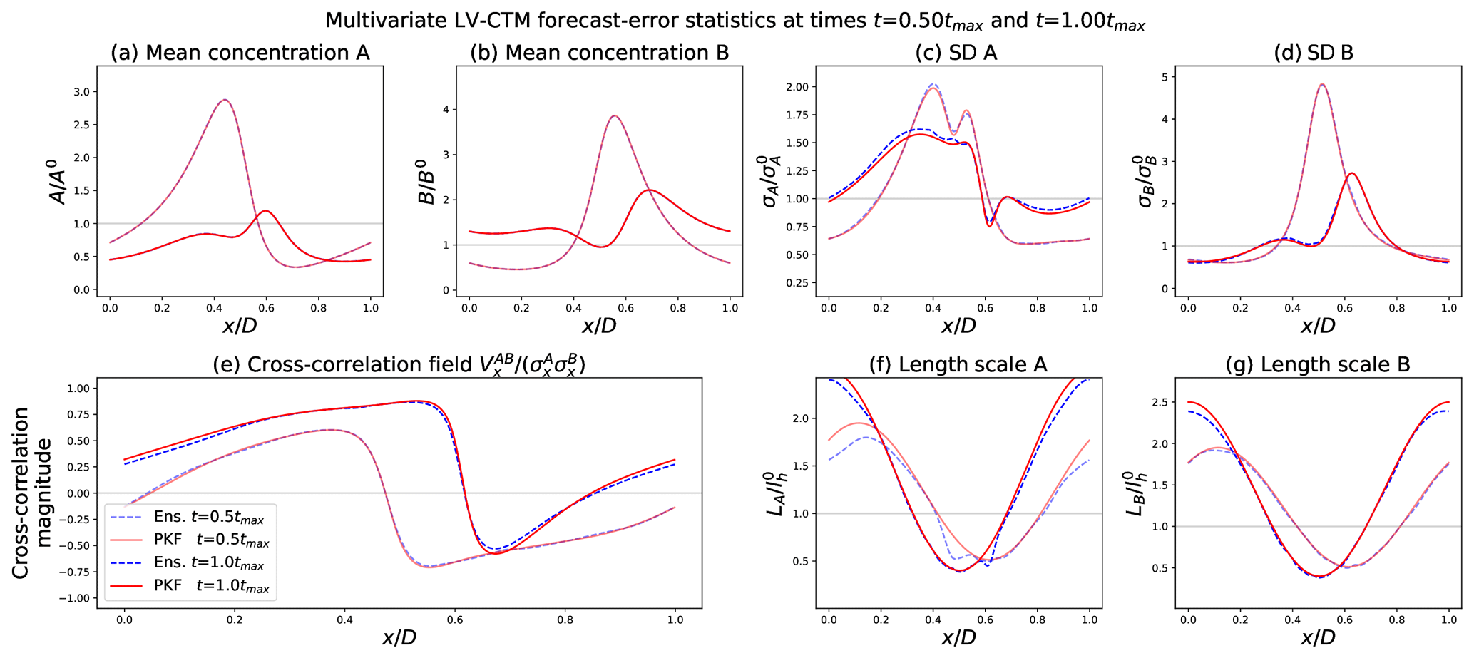
Figure 6 Results of the forecast numerical experiment. PKF error statistics (solid red lines) and EnKF-diagnosed error statistics (dashed blue lines) at times $t=[\mathrm{0.50},\mathrm{1.00}]t_{max}$. These times correspond approximately to t=23 h 45 min and t=47 h 40 min.

The forecasts of the means match perfectly for both methods (see Fig. 6a and b). Similarly to the univariate advection experiment (Sect. 2.4; see Fig. 2), an accumulation of the tracers is observed in the low-wind-speed region (centre of the domain). The standard deviations (Fig. 6c–d) observe a similar behaviour, although the effects of the chemistry appear more clearly: the curves show some quite localized deformations, especially for the standard deviation of A (compare Fig. 2b). The cross-correlation field in Fig. 6e, specific to the multivariate case, is predicted with great accuracy by the PKF dynamics. This indicates that, starting from decorrelated error fields for A and B, the chemistry dynamics have allowed non-zero cross-correlations to emerge by coupling the chemical species in a non-linear fashion. While less accurate than for the means, the filters coincide at estimating the standard deviation and for the cross-correlation fields. The forecasts of the length scales (Fig. 6f and g) show a general accordance between the two methods, even though a difference can be observed in A's case in Fig. 6f. This gap is due to the simplification of the anisotropy dynamics in the PKF formulation in Eq. (21), which does not permit such behaviours to be represented. The equation of the anisotropy dynamics of A in the original formulation of the PKF in Eq. (20f) suggests an explanation of the spikes presented on the EnKF curves in Fig. 6f which are absent for the PKF. The terms labelled T_A,chem-3 and T_A,chem-4 indicate a forcing of the spatial derivatives of the variance V_A. Looking at Fig. 6c, it appears that the variance of A presents some strong spatial heterogeneity (x=0.45 for $t=\mathrm{0.5}{t}_{max}$ and x=0.60 for $t=t_{max}$), causing important magnitudes for ∂_xV_A and thus for T_A,chem-3 and T_A,chem-4. This produces a local deformation on A's length scales which is effectively observed for the same times and locations in Fig. 6f. However, these gaps between the EnKF and PKF curves are local and of a reasonable magnitude: overall, the PKF forecast for the anisotropy reproduces the EnKF results.

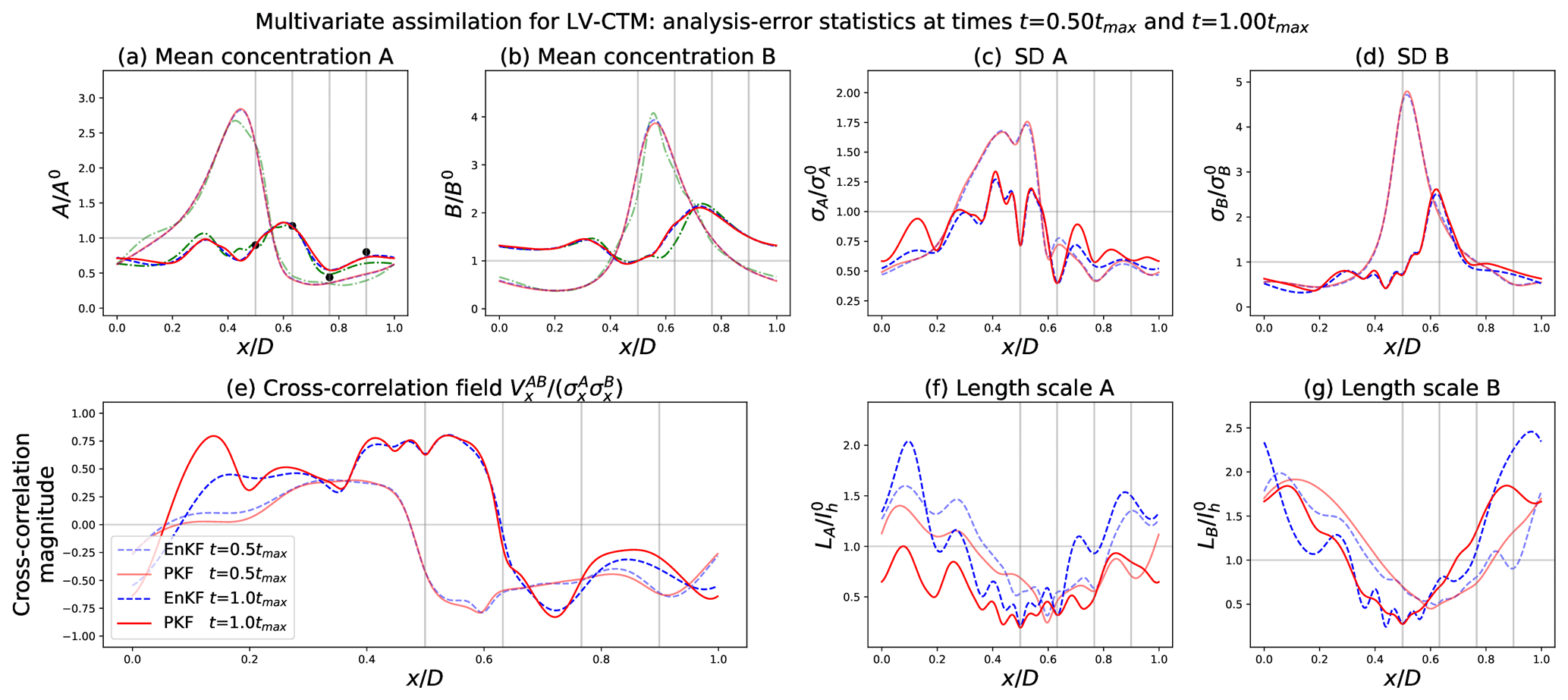
Figure 7 Results of the data assimilation numerical experiment. Nature run (dash-dotted green lines, only in panels a and b), PKF error statistics (solid red lines), and EnKF-diagnosed error statistics (dashed blue lines) at times $t=[\mathrm{0.50},\mathrm{1.00}]t_{max}$. These times correspond approximately to t=23 h 45 min and t=47 h 40 min. At time $t=\mathrm{0.5}{t}_{max}$, two analysis steps have already been performed. At time $t=\mathrm{1.00}{t}_{max}$, the fifth analysis step is being realized, and the generated observations are represented by black dots in panel (a). The vertical grey lines correspond to the sensor locations.

The outcome of the DA experiment in Fig. 7 is now shown, where five assimilation cycles are done over the period $[\mathrm{0},t_{max}]$ (one assimilation after each ${\mathit{\tau }}_{\mathrm{adv}}/\mathrm{3}$ time integration, with $t_{max}=\mathrm{5}{\mathit{\tau }}_{\mathrm{adv}}/\mathrm{3}$). The results are presented similarly to the FCST experiment, except that four vertical grey lines have been added to indicate the sensor locations. Also, time $t=t_{max}$ corresponds to a time for which synthetic observations for A are generated (see Fig. 7a).

For the DA experiment (Fig. 7), the resulting means in Fig. 7a and b are identical for the PKF and EnKF. This indicates similar forecasts and analyses for both methods during the five assimilation cycles. However, the corrections brought by the observations are not very significant given the neglected model error, the small amplitude of the forecast variance, and the observation error. This configuration implied that the generated observations are very close to the forecasted concentrations, and therefore the means are not significantly different than in the FCST experiment. The impact of the different analyses is more visible in the rest of the error statistics. For instance, the standard deviation of species A in Fig. 7c presents important downspikes which result from the uncertainty reduction during the analysis. This reduction in the uncertainty is also visible, with a reduced amplitude, in species B in Fig. 7d, for which we do not have observations. The ability to reduce the uncertainty of B and to correct its concentration when A is observed is the signature of the multivariate character of the analysis. The amplitude of the reduction in σ_B and correction of B is related to the strength of the cross-correlation at the moment of assimilation. The cross-correlation field in Fig. 7e is also impacted by the observation, but it is less obvious to say in which manner. Looking at Fig. 7f, an important gap between the PKF and EnKF for the length scales of A can be observed. It has two causes, the major one being the approximation in the anisotropy update formula in Eq. 8c. This simplified formula is less accurate than its second-order version in Eq. (10) from Pannekoucke (2021a) but offers more robustness during numerical simulations (see Fig. 13e from Pannekoucke, 2021a, and the discussion in their Sect. 4.4). The second reason is the reduction in the anisotropy dynamics to the transport process in the PKF formulation (compare Sect. 3.2). Compared to the FCST experiment, the assimilation of observations has had the effect of reducing the length scales.

In both of these experiments, the PKF has shown itself able to reproduce the results of a large ensemble Kalman filter. Again, these qualitative results of the PKF were obtained at a low numerical cost: the equivalent of 3 time integrations of Eq. (13) compared to 6400 for the EnKF.

It would be interesting to assess the robustness of the results, including whether the advection terms remain dominant under different conditions, such as weaker winds or accelerated chemistry, from a set of operational CTM predictions.

4 A more realistic chemical model: the generic reaction set (GRS) model

The simplified LV CTM has allowed for a multivariate PKF assimilation validated in numerical experiments. To explore the ability of the PKF to apply to a more complex chemical scheme, an intermediate chemical model is now introduced, the GRS (Azzi et al., 1992; Haussaire and Bocquet, 2016), which is then used to validate the PKF forecast.

4.1 Description of the GRS model

The GRS describes the dynamics of a reduced number of chemical species or pseudo species. Hence, six species are considered and interact as

$$\begin{array}{}\text{(24a)}& {\displaystyle }\text{ROC}+h\mathit{\nu }\stackrel{k_{\mathrm{1}}\left(t\right)}{\to }\text{RP}+\text{ROC},\text{(24b)}& {\displaystyle }\text{RP}+\text{NO}\stackrel{k_{\mathrm{2}}}{\to }{\mathrm{NO}}_{\mathrm{2}},\text{(24c)}& {\displaystyle }{\mathrm{NO}}_{\mathrm{2}}+h\mathit{\nu }\stackrel{k_{\mathrm{3}}\left(t\right)}{\to }\mathrm{NO}+{\mathrm{O}}_{\mathrm{3}},\text{(24d)}& {\displaystyle }\mathrm{NO}+{\mathrm{O}}_{\mathrm{3}}\stackrel{k_{\mathrm{4}}}{\to }{\mathrm{NO}}_{\mathrm{2}},\text{(24e)}& {\displaystyle }\mathrm{RP}+\mathrm{RP}\stackrel{k_{\mathrm{5}}}{\to }\mathrm{RP},\text{(24f)}& {\displaystyle }\mathrm{RP}+{\mathrm{NO}}_{\mathrm{2}}\stackrel{\mathrm{2}\cdot k_{\mathrm{6}}}{\to }\mathrm{S}\left(\mathrm{N}\right)\mathrm{GN},\end{array}$$

where ROC, RP, and S(N)GN respectively mean reactive organic compound, radical pool, and stable (non-)gaseous nitrogen product. In this chemical model, additional processes such as photolysis rate variation, ground deposits, or atmospheric emissions of certain pollutants are represented.

The system of equations of the GRS CTM is written as

$$\begin{array}{}\text{(25a)}& {\displaystyle }{\partial }_t\left[\mathrm{ROC}\right]=-{\partial }_x\left(u\cdot \left[\mathrm{ROC}\right]\right)-\mathit{\lambda }\left[\mathrm{ROC}\right]+E_{\mathrm{ROC}},\text{(25b)}& {\displaystyle }\begin{array}{rl}{\partial }_t\left[\mathrm{RP}\right]& =-{\partial }_x\left(u\cdot \left[\mathrm{RP}\right]\right)-\mathit{\lambda }\left[\mathrm{RP}\right]+k_{\mathrm{1}}\left(t\right)\left[\mathrm{ROC}\right]\\ & -\left[\mathrm{RP}\right]\left(k_{\mathrm{2}}\left[\mathrm{NO}\right]+\mathrm{2}{k}_{\mathrm{6}}\left[{\mathrm{NO}}_{\mathrm{2}}\right]+k_{\mathrm{5}}\left[\mathrm{RP}\right]\right),\end{array}\text{(25c)}& {\displaystyle }\begin{array}{rl}{\partial }_t\left[\mathrm{NO}\right]& =-{\partial }_x\left(u\cdot \left[\mathrm{NO}\right]\right)-\mathit{\lambda }\left[\mathrm{NO}\right]\\ & +E_{\mathrm{NO}}+k_{\mathrm{3}}\left(t\right)\left[{\mathrm{NO}}_{\mathrm{2}}\right]\\ & -\left[\mathrm{NO}\right]\left(k_{\mathrm{2}}\left[\mathrm{RP}\right]+k_{\mathrm{4}}\left[{\mathrm{O}}_{\mathrm{3}}\right]\right),\end{array}\text{(25d)}& {\displaystyle }\begin{array}{rl}{\partial }_t\left[{\mathrm{NO}}_{\mathrm{2}}\right]& =-{\partial }_x\left(u\cdot \left[{\mathrm{NO}}_{\mathrm{2}}\right]\right)-\mathit{\lambda }\left[{\mathrm{NO}}_{\mathrm{2}}\right]+E_{{\mathrm{NO}}_{\mathrm{2}}}\\ & +k_{\mathrm{4}}\left[\mathrm{NO}\right]\left[{\mathrm{O}}_{\mathrm{3}}\right]+k_{\mathrm{2}}\left[\mathrm{NO}\right]\left[\mathrm{RP}\right]\\ & -\left[{\mathrm{NO}}_{\mathrm{2}}\right]\left(k_{\mathrm{3}}\left(t\right)+\mathrm{2}{k}_{\mathrm{6}}\left[\mathrm{RP}\right]\right),\end{array}\text{(25e)}& {\displaystyle }\begin{array}{rl}{\partial }_t\left[{\mathrm{O}}_{\mathrm{3}}\right]& =-{\partial }_x\left(u\cdot \left[{\mathrm{O}}_{\mathrm{3}}\right]\right)-\mathit{\lambda }\left[{\mathrm{O}}_{\mathrm{3}}\right]+k_{\mathrm{3}}\left(t\right)\left[{\mathrm{NO}}_{\mathrm{2}}\right]\\ & -k_{\mathrm{4}}\left[\mathrm{NO}\right]\left[{\mathrm{O}}_{\mathrm{3}}\right],\end{array}\text{(25f)}& {\displaystyle }\begin{array}{rl}{\partial }_t\left[\mathrm{S}\left(\mathrm{N}\right)\mathrm{GN}\right]& =-{\partial }_x\left(u\cdot \left[\mathrm{S}\left(\mathrm{N}\right)\mathrm{GN}\right]\right)-\mathit{\lambda }\left[\mathrm{S}\left(\mathrm{N}\right)\mathrm{GN}\right]\\ & +\mathrm{2}{k}_{\mathrm{6}}\left[{\mathrm{NO}}_{\mathrm{2}}\right]\left[\mathrm{RP}\right],\end{array}\end{array}$$

where, for a species Z, [Z](t,x) denotes the concentration field, and for $Z\in \mathit{\{}\mathrm{ROC},\mathrm{NO},{\mathrm{NO}}_{\mathrm{2}}\mathit{\}}$, $E_Z\left(x\right)=E_Z^{\mathrm{0}}\mathit{\mu }\left(x\right)$ denotes the stationary emission field modulated by the smooth ocean–land mask $\mathit{\mu }\left(x\right)\in [\mathrm{0},\mathrm{1}]$ shown in Fig. 8b and of maximum emission $E_Z^{\mathrm{0}}$, whose value is given in Table 1 (right column). The ground deposition is represented by terms in λ, with a magnitude of 2 % d⁻¹. Kinetic parameters and chemical reaction rates are set as follows: since Eqs. (25a) and (25c) depend on the solar radiation, k₁ and k₃ evolve in time to represent the diurnal cycle, while they are related by k₁=0.152k₃ (Fig. 8c); the other rates are constant and given in Table 1.

Table 1 GRS settings.

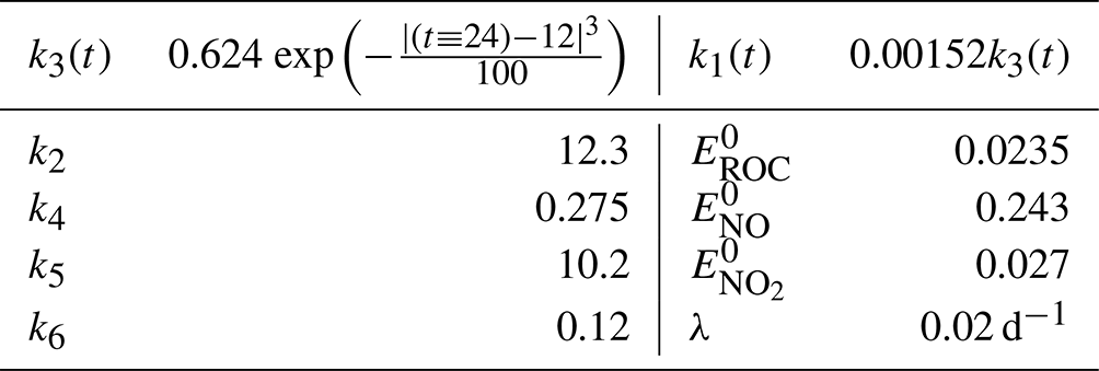
In the k₃ definition, the symbol ≡ corresponds to the modulo operator. Emission rates (ppbC d⁻¹) for ROC or (ppb d⁻¹) for NO_x and the kinetic rates (ppb⁻¹ min⁻¹), except for k₃ and k₁ (min⁻¹).

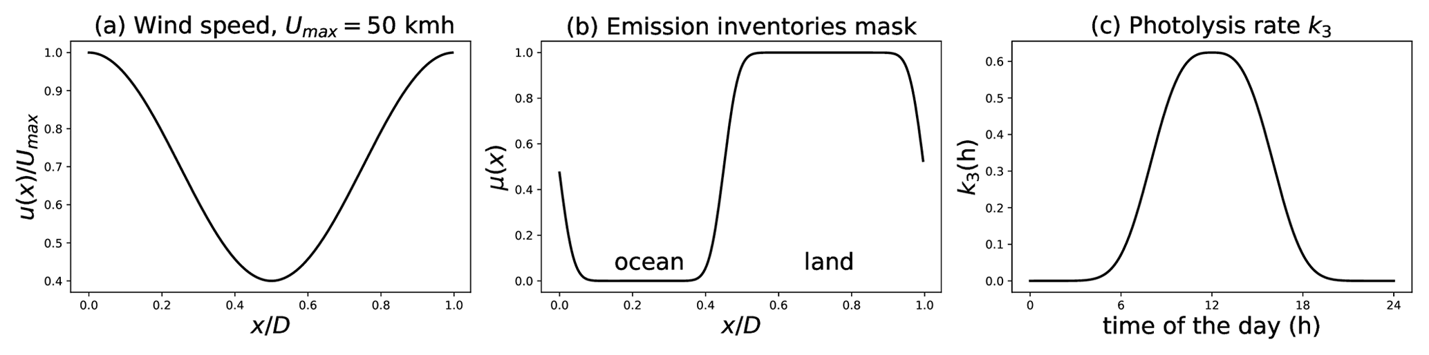
Figure 8 Settings of the GRS CTM, with the pre-defined heterogeneous and stationary wind field (a) and emission inventory mask (b) and with the diurnal cycle of the photolysis rate k₃ (min⁻¹) (c) as they are used for the simulation.

4.2 The PKF for the GRS chemical transport model

In a new numerical experiment, the PKF forecasts will be compared with those of an EnKF (of size 1600). There is no observation assimilation in this simulation.

Given the complexity of the set of Eq. (25) and the increased number of species in comparison to the LV CTM in Eq. (13), the equations of the PKF dynamics for the GRS CTM are not presented in this article but can be found in additional material (https://github.com/opannekoucke/pkf-multivariate, last access: 9 June 2023). In this context, the PKF system describes the dynamics of 33 prognostic parameters: 6 mean fields, 6 univariate variance fields, 6 anisotropy fields, and 15 cross-covariance fields (corresponding to the number of pairs of chemical species). In terms of complexity, the PKF dynamics for the GRS CTM are similar to the simplified LV CTM: the transport part is the same, while the chemical part presents the same kinds of interactions between the chemical species. However, the stationary heterogeneous emissions, not present in the LV CTM, imply a forcing in the dynamics of the mean concentrations in the GRS CTM but without an effect on the uncertainty because the emissions are not stochastic here. Note that uncertainties in emission inventories can be introduced in a PKF formulation, e.g. as a source term in the variance dynamics, and are related to the specification of boundary conditions in a PKF (Sabathier et al., 2023). Similarly to the LV CTM, the dynamics of the anisotropy are closed by removing the terms due to the chemistry. Hence, later, the dynamics of anisotropy in the GRS CTM are only due to the transport.

4.3 Numerical experiment: forecast

For the settings of this numerical experiment, the resolution of the grid has been reduced to N_x=241 grid points and the time step to $\mathrm{\Delta }t={\mathrm{10}}^{-\mathrm{4}}$ h to support the stiffness of the GRS equations. Some parameters remain unchanged: RK4 temporal scheme, finite differences to approximate spatial derivatives, choice of the wind field (Fig. 8a). The forecast starts at t₀=00 h (midnight) and ends at $t=t_{\mathrm{0}}+\mathrm{72}$ h.

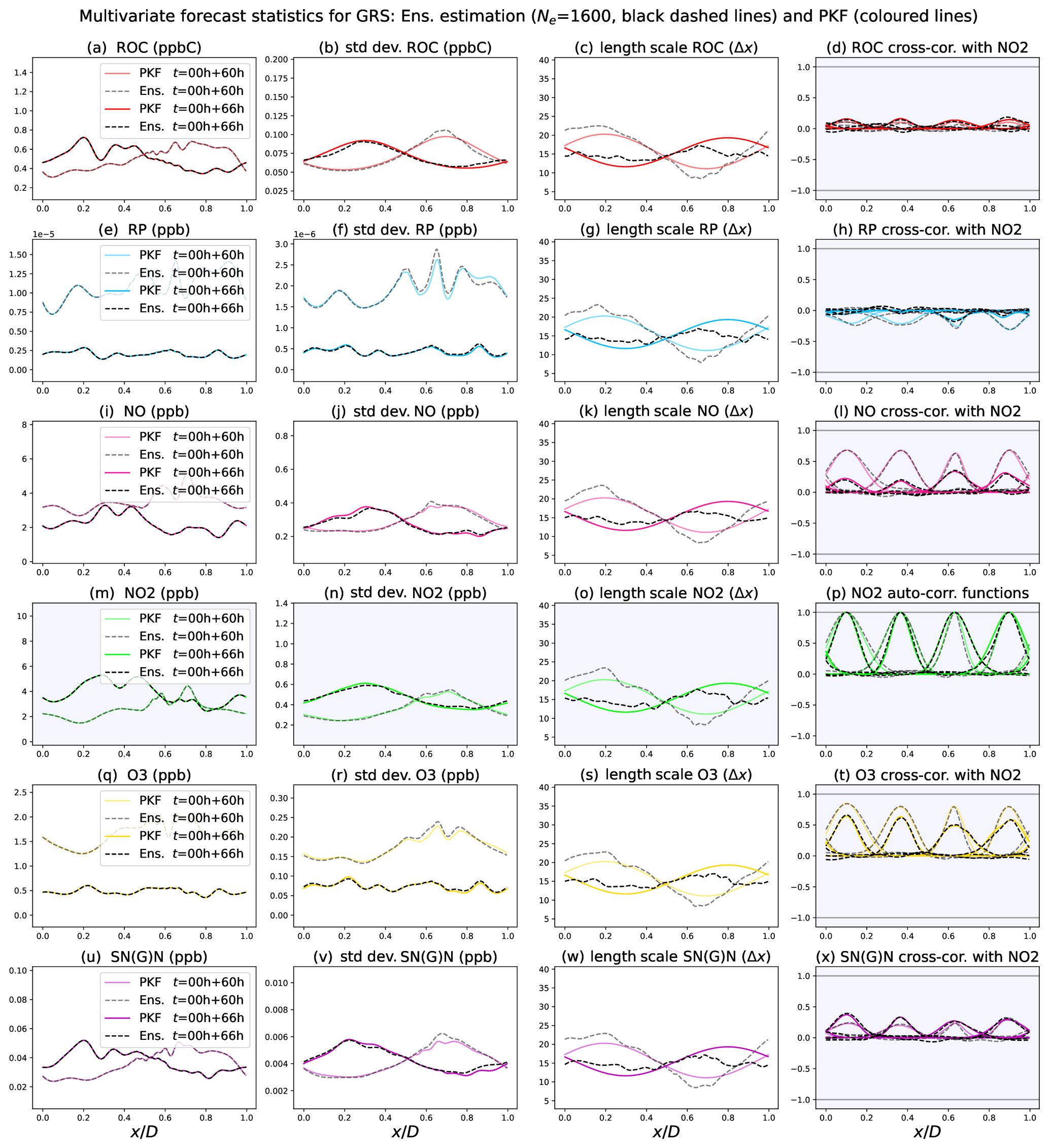
Figure 9 Multivariate forecast statistics for the GRS CTM, PKF outputs (coloured lines), and ensemble estimations from N_e=1600 forecasts (black dashed lines) for times t=00 h + {60,66} h. As we consider a simulation that starts at midnight of day 0, t=00 h + 60 h (slight transparency on the curves) corresponds to midday of day 2 and t=00 h + 66 h (no transparency) to 18:00 of day 2. From left to right, the columns correspond to the forecasts of the mean concentration, the standard deviation, the length scales (normalized by Δx), and the correlation functions (auto and cross) with NO₂ at locations $x=[\mathrm{0.1},\mathrm{0.36},\mathrm{0.63},\mathrm{0.9}]D$ for each of the six species (rows).

Realistic heterogeneous initial concentration fields are constructed as follows. First, starting from zero concentrations, a chemical equilibrium state is computed from a 4-week time integration of a 0D version of Eq. (25) where the transport has been switched off, while the concentrations are forced by their respective emissions $E_{(\cdot )}^O$. The resulting concentrations are denoted by $[Z{]}_{\mathrm{0}\mathrm{D}}^{\text{4 weeks}}$. Then, 1D concentration fields are constructed, defined as constant and equal for each species to the final value of the 0D integration. The resulting homogeneous concentration fields are then independently perturbed to produce heterogeneous concentration fields, more realistic than the homogeneous concentrations: for any species Z of the six chemical species, the resulting 1D perturbed field $\left[Z{]}^{\mathrm{0}}\right(x)=[Z{]}_{\mathrm{0}\mathrm{D}}^{\text{4 weeks}}(\mathrm{1}+\mathrm{0.15}e(x\left)\right)$, where $e={\mathbf{P}}^{\mathrm{1}/\mathrm{2}}\mathit{\zeta }$ with P, is a homogeneous Gaussian correlation version of Eq. (7) with variance 1 and constant length scale l_h=12Δx, and ζ is a sample of Gaussian random vector $\mathcal{N}(\mathrm{0},{\mathbf{I}}_{N_x})$. These perturbed 1D fields of concentrations correspond to the initial condition at t₀=00 h of the GRS-CTM simulations.

The initial condition for the PKF is set as follows. The mean state is given by the six 1D fields [Z]⁰(x). The multivariate initial uncertainty is set as univariate (no cross-correlation) with a magnitude of ${\mathit{\sigma }}^{\mathrm{0}}\left(Z\right)=\mathrm{0.15}[Z{]}_{\mathrm{0}\mathrm{D}}^{\text{4 weeks}}$ for each of the six species, with univariate homogeneous Gaussian correlation of length scale 15Δx (60 km), and the length scales are identical for all the species.

For the validation, an ensemble of 1600 initial conditions has been populated, consistently from the PKF initial conditions, by adding univariate perturbations to the GRS-CTM initial condition. For each member k of the ensemble and each field Z that is to be perturbed, $\left[Z{]}_k^{\mathrm{0}}\right(x)=[Z{]}^{\mathrm{0}}\left(x\right)+\mathrm{0.15}\left[Z{]}_{\mathrm{0}\mathrm{D}}^{\text{4 weeks}}{e}_k\right(x\left)\right)$, where $e_k={\mathbf{P}}^{\mathrm{1}/\mathrm{2}}{\mathit{\zeta }}_k$ with P is a homogeneous version of Eq. (7) with variance 1 and constant length scale l_h=15Δx and ζ is a sample of a Gaussian random vector $\mathcal{N}(\mathrm{0},{\mathbf{I}}_{N_x})$.

Figure 9 shows the statistics produced by the PKF and EnKF experiments at two instants: t=00 h + 60 h and t=00 h + 66 h. These times correspond to 12:00 and 18:00 of day 2. Each row features the uncertainty for a species Z with respectively the mean, the standard deviation, the length scale, and a selection of four cross-correlation functions with NO₂, ${\mathit{\rho }}_Z^{{\mathrm{NO}}_{\mathrm{2}}}$; this is the auto-correlation when Z is NO₂ itself. The choice of NO₂ for the cross-correlation is arbitrary, and other cross-correlations present the same behaviour (not shown).

Regarding the behaviour of the error statistics, the impact of the chemistry appears: the chemical reactions led to non-zero cross-correlations visible in the right column (except Fig. 9p, which corresponds to auto-correlations).

The impact of chemistry leads to non-zero cross-correlations between all pairs of species (Fig. 9, right column, except the auto-correlation in Fig. 9p). Also, the small-scale spatial variation, which was originally only present in the means, has been transferred to the standard-deviation fields, except for ROC. The effect of the transport is also present: it produces spatial heterogeneities in the means (left column), standard deviations (second column), and length scales (third column).

Compared to the EnKF, the PKF offers a high-quality forecast at a very low computational cost. The means (left column) are in perfect accordance in both methods. Slight differences can be observed regarding the standard-deviation fields (second column) but, as established in Sect. 2.4 (see Appendix A), the EnKF diagnoses are biased by the numerical model error that is significant when using the low-resolution grid (N_x=241 grid points in this simulation). The same argument applies to the length scales (third column), although they may also be governed by some underlying chemical dynamics similar to those described for Fig. 6f in Sect. 3.3.2). Since the PKF formulation considered here is closed by removing the contribution of the chemistry to the length-scale dynamics (following the simplification discussed in Sect. 3.2.2), the length-scale dynamics are the same for all the species. Moreover, starting from the same initial constant length-scale field l_h, the length-scale fields predicted by the PKF are the same for all the species. Nevertheless, this does not prevent the PKF from estimating the auto-correlation and cross-correlation functions (right column). The last column presents an important result: the cross-correlation function estimations by the proxy are in great accordance with the EnKF. The proxy reproduces the variety of cross-correlation functions such as negative correlations, small amplitudes, and asymmetric structures. Despite differences in length-scale estimations, the proxy shows itself to be robust and delivers satisfying modelled cross-correlation functions (at a qualitative level). This has been observed for other cross-correlation functions (not shown here). This demonstrates the capacity of the PKF to forecast the cross-covariance fields.

Note that the specific behaviour of the ROC error variance can be understood from the PKF equations for the GRS CTM (not detailed here but available on the github repository; see https://github.com/opannekoucke/pkf-multivariate/blob/master/notebooks/annexe_notebooks/computing_grs_dynamics_with_sympkf.ipynb  last access: 9 June 2023), where the dynamics of V_ROC, which read as

$$\begin{array}{}\text{(26)}& {\partial }_t{V}_{\mathrm{ROC}}+u{\partial }_x{V}_{\mathrm{ROC}}=-\mathrm{2}{V}_{\mathrm{ROC}}{\partial }_{x}u-\mathrm{2}\mathit{\lambda }{V}_{\mathrm{ROC}},\end{array}$$

are only governed by decay (term in λ) and transport (terms in u) and are not coupled with any means – while a coupling with the means is present for other chemical species. Again, this illustrates the ability of the PKF to explain the physics of uncertainties.

5 Summary and conclusions

This work explored a multivariate formulation of the PKF for atmospheric chemistry needs, when the PKF is formulated from the variance and the anisotropy tensor.

While a significant portion of the air quality uncertainty is due to meteorology (e.g. the uncertainty in the wind used for the transport), the present work focuses on the situation where the uncertainty in chemical variables is due solely to chemistry as it evolves during a given meteorological situation.

A simplified univariate chemical transport model was introduced in a 1D periodical domain with a heterogeneous wind field and conservative dynamics, illustrating the impact of the transport on the error statistics, and in particular the evolution of the variance and of the anisotropy (length scale) due to the wind heterogeneity. Compared with an estimation from a large ensemble of 6400 forecasts, the PKF has proven to be able to reproduce the variance and the anisotropy and also able to provide a proxy for the correlation functions. The PKF prediction has been obtained at a lower numerical cost compared with the cost of the ensemble. In addition, the PKF has been shown to be less sensitive to a dispersive model error encountered for this simulation that required computation of the ensemble at a high resolution to mitigate the effect of the dispersive term on the ensemble estimation. This simplified model proposed a proxy for multivariate covariance to approximate cross-covariances, which extends the univariate covariance model parameterized from variance and anisotropy, but the resulting multivariate covariance is symmetric with no guarantee of positiveness.

Then a simplified multivariate chemical transport model was introduced to tackle multivariate error statistics. Based on Lotka–Volterra (LV) dynamics, this test bed reproduces non-linear coupling between chemical species and the transport due to the wind, as it can be observed in a real chemical transport model. Then a multivariate PKF formulation was proposed, which made a closure issue related to the chemical part appear, but not to the transport, and concerns the dynamics of the anisotropy. A detailed analysis of the effect of the chemistry on the dynamics of the anisotropy led to an analytical solution of the multivariate evolution of the uncertainty in a 1D harmonic oscillator, which helps to understand the transfer of uncertainty from one species to another.

The PKF has permitted the understanding of the uncertainty dynamics: it offered equations that described the time evolutions of variances, cross-covariances, and anisotropies. The impacts of the advection and the chemistry have been clearly identified in the dynamics of the error statistics, allowing for a better comprehension of the overall problem. Since the relative contribution of the transport was larger than the one of the chemistry in the trend of the anisotropy, a closed form has been considered by removing the terms related to the chemistry in the dynamics of the anisotropy.

Despite this approximation, a validation test bed using an ensemble method showed that the PKF dynamics are able to predict the uncertainty dynamics for two chemical schemes based on LV. Moreover, a multivariate formulation of the PKF analysis step has been introduced, given by Algorithm F1, and several assimilation cycles have been conducted for the LV chemical scheme, showing that a multivariate PKF assimilation is possible, which is promising.

A final multivariate example, focused on the forecast step, was introduced to evaluate the potential of the multivariate PKF formulation to a larger system. In this case, the chemical scheme (GRS) describes the interaction of six species. Again, this example has shown the ability of the PKF to reproduce the EnKF error statistics.

To go further, it will be interesting to see whether the advection terms remain dominant under different conditions like weaker wind or accelerated chemistry from an ensemble of forecasts of operational CTMs, where isotropic and homogeneous correlations are often considered in variational data assimilation.

In addition, since we have focused on the uncertainty due to chemistry, it would be interesting to address the part of the uncertainty due to meteorology. For a CTM like MOCAGE, this could be done by considering an ensemble of weather forecasts with each member used as a forcing for a single CTM forecast. However, this solution would lead to multiple CTM forecasts, which would be expensive. Therefore, from the perspective of using a PKF (applied to a CTM), a less expensive solution would be to consider a single PKF forecast where the wind is uncertain (stochastic advection wind), with the wind uncertainty characterized by the variance and the anisotropy tensor estimated from the weather forecast ensemble. The challenge will be to find an appropriate closure for the unknown terms in the dynamics, including the cross-correlation between the wind error and chemical species, with the help of this contribution to multivariate statistics.

This work is a milestone in the development of a multivariate assimilation based on the PKF and applied to air quality and is an important step in extending the univariate PKF implementation to complex operational CTMs like the operational transport model MOCAGE at Météo-France. The work also highlights a drawback of the PKF: the cost of the current multivariate PKF formulation scales as the square of number of chemical species, which appears to be a limitation, at least if all the chemical species are considered in the multivariate uncertainty prediction. Hence, it would be interesting to test a PKF formulation on a reduced chemical scheme of interest for the data assimilation.

Moreover, while this contribution focused on air quality, it contributes to improving our understanding of multivariate statistics, e.g. with the analytical solution of the 1D harmonic oscillator. It would be interesting to extend this multivariate PKF formulation to other geophysical applications, e.g. numerical weather prediction, with particular attention paid to the extension of the multivariate cross-covariance proxy to the 2D or 3D domains. Compared with air quality where the chemical reactions are point-wise, geophysical equations make local interactions appear that have to be studied in view of the PKF approach, e.g. the geostrophic balance in the barotropic model.

Appendix A: Limits of the numerical validation of the PKF in the presence of model error

The exploration of the uncertainty dynamics from numerical experiments, as made here to validate the PKF from an ensemble method, faces some limits. Figure 2 has shown a gap between the PKF and EnKF regarding the forecast of the error statistics (standard deviation in Fig. 2b and length scales in Fig. 2c). We now justify this observation, relating it to a model error.

As the problem is discretized for numerical simulations, the actual equation that is simulated is not exactly Eq. (9a) but rather an implicit modified equation induced by the use of finite differences for the spatial and temporal discretizations. Focusing on the spatial discretization, the modified equation is written as

$$\begin{array}{}\text{(A1)}& \begin{array}{rl}{\partial }_t\mathcal{X}& =-u{\partial }_x\mathcal{X}-\mathcal{X}{\partial }_{x}u-{\displaystyle \frac{\mathrm{\Delta }{x}^{\mathrm{2}}}{\mathrm{6}}}u{\partial }_x^{\mathrm{3}}\mathcal{X}\\ & -{\displaystyle \frac{\mathrm{\Delta }{x}^{\mathrm{2}}}{\mathrm{6}}}\mathcal{X}{\partial }_x^{\mathrm{3}}u+\mathcal{O}\left(\mathrm{\Delta }{x}^{\mathrm{3}}\right),\end{array}\end{array}$$

which shows additional dispersive terms not present in the initial dynamics (Eq. 9a). Note that Eq. (A1) is not the full modified equation of the discretized model: in particular, it does not represent the effect of the RK4 time scheme, but the error associated with the fourth-order time scheme should be negligible compared with the spatial numerical error (second-order). Hence, Eq. (A1) should be close to the true modified equation, and the presence of additional processes may explain the significant differences observed in Fig. 2b and c: the dispersive term $-\frac{\mathrm{\Delta }{x}^{\mathrm{2}}}{\mathrm{6}}u{\partial }_x^{\mathrm{3}}\mathcal{X}$ contributes to reducing the speed of the transport to a value lower than u, while the term $-\frac{\mathrm{\Delta }{x}^{\mathrm{2}}}{\mathrm{6}}\mathcal{X}{\partial }_x^{\mathrm{3}}u$ implies a local exponential growing (damping) of 𝒳(t,x), where ${\partial }_x^{\mathrm{3}}u$ is negative (positive). This exponential evolution only contributes to the magnitude of the forecast error: i.e. it modifies the variance field, but it has no influence on the length scale (Pannekoucke et al., 2018). At the opposite end, the dispersive term influences both the variance and the length scale, as can be observed in Fig. 2c: the EnKF curves appear slightly late behind the PKF ones (the wind transports the curves toward the right), presenting a negative shift in the amplitude.

This can be understood as follows. Since Eq. (A1) is linear, it is the dynamics of the mean and of the errors in the numerical experiment. However, the typical scales of the mean and of the error are different: in this simulation, the spatial scale of the mean state is large, of order D, while the spatial scale of the errors is of order $l_{\mathrm{h}}\approx D/\mathrm{16}$, where $\mathrm{16}\approx \mathrm{241}/\mathrm{15}$; this implies that the magnitude of the negative phase shift due to the dispersive term is larger for the error than for the mean (see e.g. Korteweg–de Vries (KdV) Eq. 1.19 in Whitham, 1999, p. 9).

This justifies why the dispersion does not affect the prediction of the mean state – the estimation for the means coinciding for the two methods in Fig. 2a –, while it acts on the EnKF predictions of the variance and of the length scale, related to the error dynamics. In this simulation, the PKF in Eq. (10) is not influenced by the dispersion because the spatial scale of the variance and of the length-scale fields is large (order of D). This points out the sensitivity of the EnKF to numerical model error.

Since the magnitude of the dispersive term scales as 𝒪(Δx²), a simulation at high resolution could damp this term and would lead to attributing the gap observed in Fig. 2 to the model error.

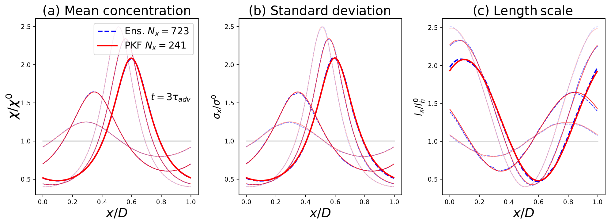
Figure A1 Same experiment as Fig. 2 except that the EnKF forecast has been simulated using a higher grid definition (N_x=723) to reduce numerical model error.

This is demonstrated by comparing the PKF statistics to a high-resolution forecast of the EnKF with a grid of 3 times the original resolution, i.e. $N_x=\mathrm{3}\times \mathrm{241}=\mathrm{723}$ grid points. To be consistent with the initial low-resolution experiment, the initial length scale of the high resolution is set to $l_{\mathrm{h}}^{\mathrm{0}}=\mathrm{3}\times \mathrm{15}\mathrm{\Delta }x=\mathrm{45}\mathrm{\Delta }x\simeq \mathrm{62.2}$ km. The time step has been adapted in consequence to match the CFL condition. The results of this new simulation, in Fig. A1, show that predicting the ensemble at high resolution leads to the same variance (Fig. A1b) and length-scale (Fig. A1c) fields as the ones predicted by the PKF, while the latter is computed at low resolution. A PKF at high resolution has been computed (not shown here) and has been found to be equivalent to the PKF computed at low resolution, with a relative error at the end of the forecast window of lower than 0.2 % for the mean, 0.3 % for the standard deviation, and 0.05 % for the length scale, where the relative error of fields has been computed as $\left|\right|{\mathrm{PKF}}_{\mathrm{LR}}-{\mathrm{PKF}}_{\mathrm{HR}}\left|\right|/\left|\right|{\mathrm{PKF}}_{\mathrm{HR}}\left|\right|$, with the L2 functional norm defined for a function f as $\left|\right|f\left|\right|=\sqrt{\int f^{\mathrm{2}}\left(x\right)dx}$ . This demonstrates the quality of the forecasted error statistics for the PKF, even at a low resolution. Figure B1 also shows the correlation functions computed from the high-resolution EnKF forecast. The correlation functions represented are in better accordance with the PKF-modelled correlation functions than for the low-resolution ensemble forecast: see e.g. Fig. B1d to f. This shows that the PKF is little subject to numerical model error as the error-statistic forecasts directly result from their time integration. Compared to previous studies that focused only on the comparison of variance and anisotropy error statistics, here we have shown the ability to reproduce complex heterogeneous correlation functions using the PKF formulation in the 1D domain.

Appendix B: Validation of correlation functions in univariate situations

Figure B1 compares the correlation functions at position x_l=0.5, estimated from the ensemble for the EnKF and modelled from the predicted parameters for the PKF when using Eq. (7), at different times. At a qualitative level, the PKF is able to approximate the correlation functions, the latter being only known to within a sampling noise because of the ensemble estimation which is assumed to be low due to the ensemble size. In particular, the PKF is able to reproduce the large (small) spread of the symmetric correlations present in Fig. B1a (Fig. B1b). However, the PKF is also able to represent the anisotropy of the correlations, such as the one shown e.g. in Fig. B1e, where the correlation function at that time appears broader in its right-hand part (corresponding to x larger than x_l) than in its left-hand part (corresponding to x smaller than x_l).

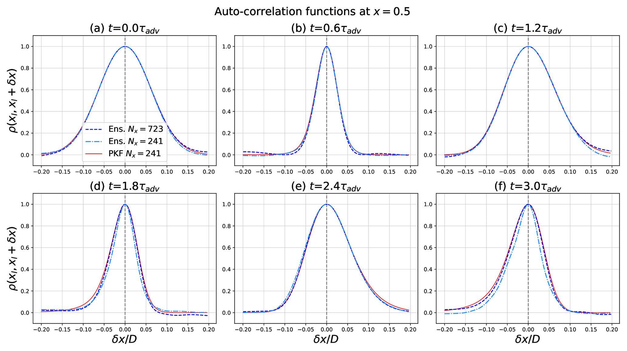
Figure B1 Correlation functions at location x_l=0.5 and times $t=[\mathrm{0.0},\mathrm{0.6},\mathrm{1.2},\mathrm{1.8},\mathrm{2.4},\mathrm{3.0}]{\mathit{\tau }}_{\mathrm{adv}}$, computed with PKF correlation model fitted with a low-resolution (N_x=241) PKF forecast for error statistics (red lines) and diagnosed on the low-resolution (N_x=241) ensemble (cyan dash-dotted lines) and high-resolution (N_x=723) ensemble (blue dashed lines), of ensemble size N_e=6400.

Appendix C: Lotka–Volterra chemical model

We consider four chemical species $A,B,X$, and Y governed by the chemical reactions

$$\begin{array}{}\text{(C1)}& {\displaystyle }X+A\stackrel{k_{\mathrm{1}}}{\to }\mathrm{2}A,\text{(C2)}& {\displaystyle }A+B\stackrel{k_{\mathrm{2}}}{\to }\mathrm{2}B,\text{(C3)}& {\displaystyle }B\stackrel{k_{\mathrm{3}}}{\to }Y.\end{array}$$

The kinetics of the reaction, deduced from the mass action law for reaction rates, are written as

$$\begin{array}{}\text{(C4a)}& {\displaystyle \frac{\mathrm{d}\left[A\right]}{\mathrm{d}t}}& {\displaystyle }=k_{\mathrm{1}}\left[X\right]\left[A\right]-k_{\mathrm{2}}\left[A\right]\left[B\right],\text{(C4b)}& {\displaystyle \frac{\mathrm{d}\left[B\right]}{\mathrm{d}t}}& {\displaystyle }=k_{\mathrm{2}}\left[A\right]\left[B\right]-k_{\mathrm{3}}\left[B\right],\end{array}$$

where [⋅] denotes the concentration. When the concentrations of X and Y are constant, the system simplifies as

$$\begin{array}{}\text{(C5a)}& {\displaystyle \frac{\mathrm{d}\left[A\right]}{\mathrm{d}t}}& {\displaystyle }=k_{\mathrm{1}}\left[A\right]-k_{\mathrm{2}}\left[A\right]\left[B\right],\text{(C5b)}& {\displaystyle \frac{\mathrm{d}\left[B\right]}{\mathrm{d}t}}& {\displaystyle }=k_{\mathrm{2}}\left[A\right]\left[B\right]-k_{\mathrm{3}}\left[B\right],\end{array}$$

which is a Lotka–Volterra system.

Appendix D: Contribution of the chemistry to the uncertainty dynamics in the LV CTM

This section contributes to evaluating the impact of chemistry on the dynamics of uncertainty with respect to the effect due to advection, leading to a closure for the PKF applied to the multivariate LV CTM.

D1 Impact of the chemistry alone on the dynamics of the anisotropies for homogeneous statistical initial conditions

Regarding the dynamics of the anisotropy fields presented in the prognostic equations (Eqs. 20f–20g), the part due to transport in $T_{\text{adv-}(\cdot )}^{(\cdot )}$ is already well understood, as it comes down to the univariate case presented in Sect. 2.4. However, the role of the chemistry in $T_{\text{chem-}(\cdot )}^{(\cdot )}$ is unclear at this time. The transport process is removed to focus on the dynamics of the anisotropy due to the chemistry.

In the PKF dynamics in Eq. (20), when there is no transport and when the variance fields are homogeneous at the initial condition, the homogeneity is preserved during the time evolution. Hence, the spatial derivatives of the variance and of the cross-variance fields are null, which leads to simplification of the dynamics of the anisotropy (Eqs. 20f–20g) as

$$\begin{array}{}\text{(D1a)}& {\displaystyle }{\partial }_t{s}_A& {\displaystyle }={\displaystyle \frac{\mathrm{2}{k}_{\mathrm{2}}A{s}_A}{{\mathit{\sigma }}_A}}\left({\mathit{\sigma }}_B{s}_A\stackrel{\mathrm{‾}}{{\partial }_x{\stackrel{\mathrm{̃}}{\mathit{\epsilon }}}_A{\partial }_x{\stackrel{\mathrm{̃}}{\mathit{\epsilon }}}_B}-{\displaystyle \frac{V_{AB}}{{\mathit{\sigma }}_A}}\right),\text{(D1b)}& {\displaystyle }{\partial }_t{s}_B& {\displaystyle }={\displaystyle \frac{\mathrm{2}{k}_{\mathrm{2}}B{s}_B}{{\mathit{\sigma }}_B}}\left({\displaystyle \frac{V_{AB}}{{\mathit{\sigma }}_B}}-{\mathit{\sigma }}_A{s}_B\stackrel{\mathrm{‾}}{{\partial }_x{\stackrel{\mathrm{̃}}{\mathit{\epsilon }}}_A{\partial }_x{\stackrel{\mathrm{̃}}{\mathit{\epsilon }}}_B}\right).\end{array}$$

To focus on the contribution of the chemistry to the dynamics of the anisotropies, an ensemble of N_e=1600 high-resolution forecasts is performed (N_x=723) with only the chemistry part. Hence, the transport terms are set to zero in Eq. (13). Two numerical experiments are conducted: first, the initial length scales are equal for both species, with $l_A^{\mathrm{0}}=l_B^{\mathrm{0}}=\mathrm{45}\mathrm{\Delta }x\simeq \mathrm{62}$ km (results are shown in Fig. D1), and are then different with $l_A^{\mathrm{0}}=\mathrm{45}\mathrm{\Delta }x$ and $l_B^{\mathrm{0}}=\mathrm{66}\mathrm{\Delta }x\simeq \mathrm{91}$ km (results in Fig. D2). The initial conditions for the concentrations and the multivariate statistics are chosen to be homogeneous over the domain in both cases. Therefore, only the time series of the spatial average are shown for the variance, the cross-correlation, the length scale, and the open term $\stackrel{\mathrm{‾}}{{\partial }_x{\stackrel{\mathrm{̃}}{\mathit{\epsilon }}}_A{\partial }_x{\stackrel{\mathrm{̃}}{\mathit{\epsilon }}}_B}$, which is estimated from the ensemble by

$$\begin{array}{}\text{(D2)}& \widehat{{\partial }_x{\stackrel{\mathrm{̃}}{\mathit{\epsilon }}}_A{\partial }_x{\stackrel{\mathrm{̃}}{\mathit{\epsilon }}}_B}={\displaystyle \frac{\mathrm{1}}{N_{\mathrm{e}}}}\sum _{k=\mathrm{1}}^{N_{\mathrm{e}}}{\partial }_x{\stackrel{\mathrm{̃}}{\mathit{\epsilon }}}_{A,k}{\partial }_x{\stackrel{\mathrm{̃}}{\mathit{\epsilon }}}_{B,k},\end{array}$$

where ${\stackrel{\mathrm{̃}}{\mathit{\epsilon }}}_{A,k}={\mathit{\epsilon }}_{A,k}/{\widehat{V}}_A$ and ${\stackrel{\mathrm{̃}}{\mathit{\epsilon }}}_{B,k}={\mathit{\epsilon }}_{B,k}/{\widehat{V}}_B$.

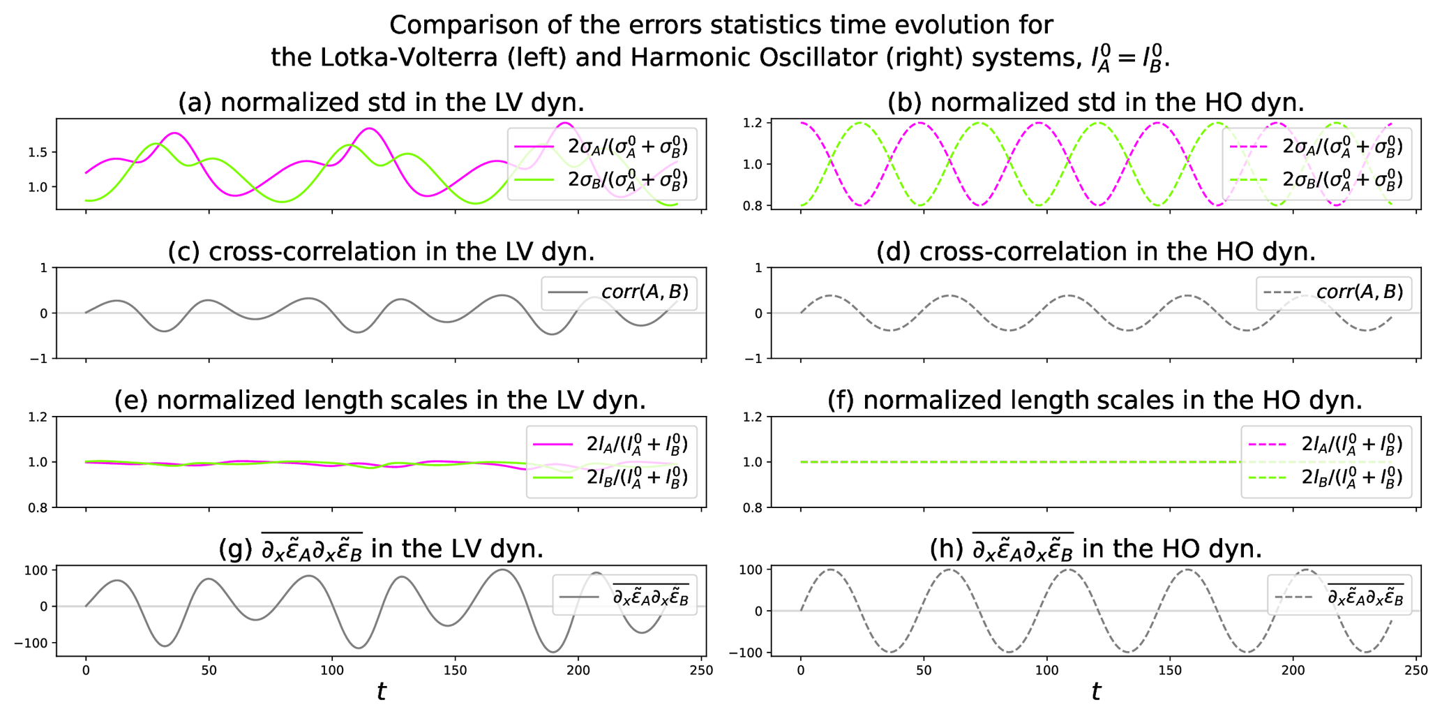
Figure D1 Time series of the spatial average of the error statistics from the ensemble forecast with N_e=1600 for Lotka–Volterra (LV, left column) and harmonic oscillator analytical solutions (HO, right column). Equal initial length scales: $l_A^{\mathrm{0}}=l_B^{\mathrm{0}}=\mathrm{45}\mathrm{\Delta }x$.

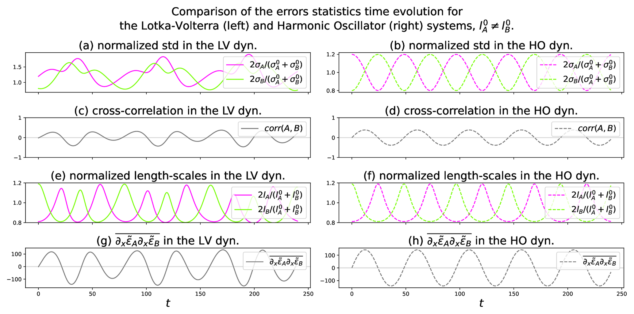
Figure D2 Time series of the spatial average of the error statistics from the ensemble forecast with N_e=1600 for LV (left column) and HO analytical solutions (right column). Different initial length scales: $l_A^{\mathrm{0}}=\mathrm{45}\mathrm{\Delta }x$ and $l_B^{\mathrm{0}}=\mathrm{66}\mathrm{\Delta }x$.

In the first experiment, Fig. D1, the magnitude of the error, given by the standard deviations in Fig. D1a, oscillates with a phase shift where the magnitude of the error in A advances the one of B. The cross-correlation in Fig. D1c and the unclosed term $\stackrel{\mathrm{‾}}{{\partial }_x{\stackrel{\mathrm{̃}}{\mathit{\epsilon }}}_A{\partial }_x{\stackrel{\mathrm{̃}}{\mathit{\epsilon }}}_B}$ in Fig. D1g oscillate in a similar way. In this experiment, where the initial length scales are identical for A and B, there is no time evolution of the length scales, except the fluctuations that are due to the sampling noise (see Fig. D1e). The second experiment, Fig. D2, shows roughly the same picture, except that, this time, with initial length scales of different values, oscillations appear (Fig. D2e). Since, a priori, it is not easy to track the reason for the change in behaviour observed in the length-scale dynamics, an analytical investigation of the harmonic oscillator (HO),

$$\begin{array}{}\text{(D3a)}& {\displaystyle }{\partial }_{t}A(t,\mathit{x})=-kB(t,\mathit{x}),\text{(D3b)}& {\displaystyle }{\partial }_{t}B(t,\mathit{x})=kA(t,\mathit{x}),\end{array}$$

is introduced, with k=k₂. The comparison with HO is relevant since it is an example of analytical multivariate dynamics and also because it mimics the periodic oscillations of LV, explaining the numerical results. For HO, it is possible to calculate the time evolution of the statistics analytically (see Appendix E for details), which is written as

$$\begin{array}{}\text{(D4a)}& {\displaystyle }{V}_A\left(t\right)=\cos (kt{)}^{\mathrm{2}}{V}_A^{\mathrm{0}}+\sin (kt{)}^{\mathrm{2}}{V}_B^{\mathrm{0}},\text{(D4b)}& {\displaystyle }{V}_B\left(t\right)=\sin (kt{)}^{\mathrm{2}}{V}_A^{\mathrm{0}}+\cos (kt{)}^{\mathrm{2}}{V}_B^{\mathrm{0}},\text{(D4c)}& {\displaystyle }{V}_{AB}\left(t\right)=\cos \left(kt\right)\sin \left(kt\right)\left(V_A^{\mathrm{0}}-V_B^{\mathrm{0}}\right),\text{(D4d)}& {\displaystyle }{s}_A\left(t\right)=V_A\left(t\right){\left[\cos (kt{)}^{\mathrm{2}}{\displaystyle \frac{V_A^{\mathrm{0}}}{s_A^{\mathrm{0}}}}+\sin (kt{)}^{\mathrm{2}}{\displaystyle \frac{V_B^{\mathrm{0}}}{s_B^{\mathrm{0}}}}\right]}^{-\mathrm{1}},\text{(D4e)}& {\displaystyle }{s}_B\left(t\right)=V_B\left(t\right){\left[\sin (kt{)}^{\mathrm{2}}{\displaystyle \frac{V_A^{\mathrm{0}}}{s_A^{\mathrm{0}}}}+\cos (kt{)}^{\mathrm{2}}{\displaystyle \frac{V_B^{\mathrm{0}}}{s_B^{\mathrm{0}}}}\right]}^{-\mathrm{1}},\text{(D4f)}& {\displaystyle }\stackrel{\mathrm{‾}}{{\partial }_x{\stackrel{\mathrm{̃}}{\mathit{\epsilon }}}_A{\partial }_x{\stackrel{\mathrm{̃}}{\mathit{\epsilon }}}_B}\left(t\right)={\displaystyle \frac{\cos \left(kt\right)\sin \left(kt\right)}{{\mathit{\sigma }}_A\left(t\right){\mathit{\sigma }}_B\left(t\right)}}\left[{\displaystyle \frac{V_A^{\mathrm{0}}}{s_A^{\mathrm{0}}}}-{\displaystyle \frac{V_B^{\mathrm{0}}}{s_B^{\mathrm{0}}}}\right].\end{array}$$

Numerical results computed for the HO are represented in Fig. D1 and Fig. D2 and show some of the behaviour encountered for the non-linear LV equations. For instance, the oscillations of the variance are visible. Moreover, the length scales oscillate depending on the initial condition: when the initial length scales are equal, there is no oscillation (see Fig. D1f) that appears from the analytical computation of s_A and s_B; in contrast, for different values of the initial length scales, oscillations appear (see Fig. D2f). These different behaviours of the anisotropy based on the initial settings of the length scales are explained by the analytical solutions of the error statistics for the harmonic oscillator. For instance, when plugging the identical initial condition for the length scales $s_A^{\mathrm{0}}=s_B^{\mathrm{0}}$ and the analytical solution of V_A(t) (Eq. D4a) into the right-hand side of Eq. (D4d), it simplifies to $s_A\left(t\right)=s_A^{\mathrm{0}}$. The same result applies for s_B(t). This simplification no longer holds when $C\ne s_B^{\mathrm{0}}$, leading to non-constant length scales which are effectively observed.

Figure D3 Numerical results for the case $l_A^{\mathrm{0}}=l_B^{\mathrm{0}}=\mathrm{45}\mathrm{\Delta }x$. Time evolution for the relative contribution by term (process) computed from Eq. (D6) (Eq. D7) involved in the anisotropy dynamics for species A and B in panels (a) and (b) (panels c and d).

Figure D4 Numerical results for the cases $l_A^{\mathrm{0}}=\mathrm{45}\mathrm{\Delta }x$ and $l_B^{\mathrm{0}}=\mathrm{66}\mathrm{\Delta }x$. Time evolution for the relative contribution by term (process) computed from Eq. D6 (Eq. D7) involved in the anisotropy dynamics for species A and B in panels (a) and (b) (panels c and d).

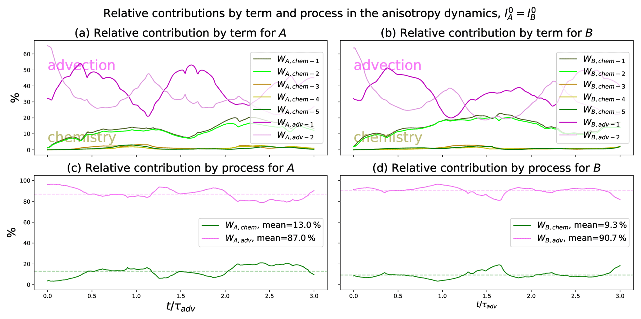
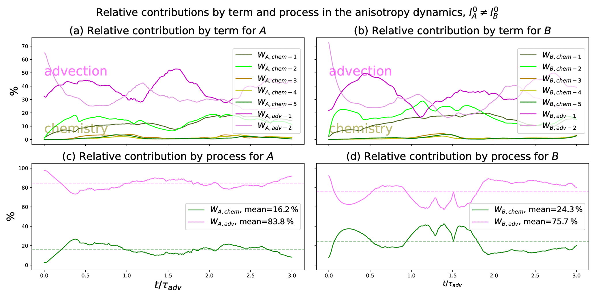
Note that, for equal initial length scales, the anisotropy appears to be stationary (see Fig. D1e), which suggests a closure for the open term $\stackrel{\mathrm{‾}}{{\partial }_x{\stackrel{\mathrm{̃}}{\mathit{\epsilon }}}_A{\partial }_x{\stackrel{\mathrm{̃}}{\mathit{\epsilon }}}_B}$: since the anisotropy is equal and constant, $s_A\left(t\right)=s_B\left(t\right)=\frac{s_A\left(t\right)+s_B\left(t\right)}{\mathrm{2}}=s_A^{\mathrm{0}}=s_B^{\mathrm{0}}=\frac{s_A^{\mathrm{0}}+s_B^{\mathrm{0}}}{\mathrm{2}}$; then, from the stationarity of the anisotropy, ${\partial }_t{s}_A={\partial }_t{s}_B=\mathrm{0}$, the right-hand side of Eq. (D1) leads to the expression

$$\begin{array}{}\text{(D5)}& \stackrel{\mathrm{‾}}{{\partial }_x{\stackrel{\mathrm{̃}}{\mathit{\epsilon }}}_A{\partial }_x{\stackrel{\mathrm{̃}}{\mathit{\epsilon }}}_B}={\displaystyle \frac{V_{AB}\left(x\right)}{{\mathit{\sigma }}_A\left(x\right){\mathit{\sigma }}_B\left(x\right)}}{\displaystyle \frac{\mathrm{2}}{s_A\left(x\right)+s_B\left(x\right)}}.\end{array}$$

This closure indicates that the term $\stackrel{\mathrm{‾}}{{\partial }_x{\stackrel{\mathrm{̃}}{\mathit{\epsilon }}}_A{\partial }_x{\stackrel{\mathrm{̃}}{\mathit{\epsilon }}}_B}$ is proportional to the cross-correlation in this particular case. This is confirmed in Fig. D1, where $\stackrel{\mathrm{‾}}{{\partial }_x{\stackrel{\mathrm{̃}}{\mathit{\epsilon }}}_A{\partial }_x{\stackrel{\mathrm{̃}}{\mathit{\epsilon }}}_B}$ in Fig. D1g appears to evolve as the cross-correlation in Fig. D1c. For this specific case, Eq. (D5) also applies for the error statistics of the harmonic oscillator: using $s_A^{\mathrm{0}}=s_B^{\mathrm{0}}$ and the time evolution of the cross-covariance V_AB (Eq. D4c) allows us to solve for the open term in Eq. (D4f), obtaining the same expression as in Eq. (D5).

The time evolution of the HO error statistics makes an alternate transfer of the error statistics appear between the two components A and B, which qualitatively reproduces the evolution observed in the LV dynamics. The transfer of uncertainty from one component to the other is provided by the cross-covariance V_AB when the error variance is different for each of the two species.

D2 Detailed contribution of each process to the dynamics of the anisotropy

The following section aims at identifying the dominant terms or processes in the dynamics of the anisotropy (Eqs. 20f and 20g).

Two different evaluations are performed. The first one evaluates the relative contribution W_Z,j of the term T_Z,j with respect to all other terms in the dynamics of the anisotropy of Z, which reads as

$$\begin{array}{}\text{(D6)}& W_{Z,j}\left(t\right)={\displaystyle \frac{\left|\right|T_{Z,j}\left(t\right)|{|}_{\mathrm{1}}}{{\sum }_k\left|\right|T_{Z,k}\left(t\right)|{|}_{\mathrm{1}}}},\end{array}$$

where $\left|\right|v|{|}_{\mathrm{1}}=\frac{\mathrm{1}}{N_x}{\sum }_{j=\mathrm{1},\mathrm{\dots },Nx}|v_j|$ is the L¹ norm on the discretized domain [0,D). The second one evaluates the relative contribution of each physical processes in the dynamics of the anisotropy e.g. the relative contribution of the advection in the dynamics of the anisotropy of Z, W_Z,adv, reads as

$$\begin{array}{}\text{(D7)}& \begin{array}{rl}& W_{Z,\mathrm{adv}}\left(t\right)=\\ & {\displaystyle \frac{\left|\right|{\sum }_{k=\mathrm{1}}^{\mathrm{2}}{T}_{Z,\mathrm{adv}-k}\left(t\right)|{|}_{\mathrm{1}}}{\left|\right|{\sum }_{k=\mathrm{1}}^{\mathrm{2}}{T}_{Z,\mathrm{adv}-k}\left(t\right)|{|}_{\mathrm{1}}+|\left|{\sum }_{k=\mathrm{1}}^{\mathrm{5}}{T}_{Z,\mathrm{chem}-k}\right(t\left)\right|{|}_{\mathrm{1}}}},\end{array}\end{array}$$

from which the relative contribution of the chemistry is written as $W_{Z,\mathrm{chem}}\left(t\right)=\mathrm{1}-W_{Z,\mathrm{adv}}\left(t\right)$. Note that the normalization is different between Eqs. (D6) and (D7).

The computation of these relative contributions will rely on ensemble of forecasts. They will be used to diagnose a posteriori the PKF parameters $(A,B,V_A,V_B,V_{AB},s_A,s_B)$ as well as the three open terms $(\stackrel{\mathrm{‾}}{{\partial }_x{\stackrel{\mathrm{̃}}{\mathit{\epsilon }}}_A{\partial }_x{\stackrel{\mathrm{̃}}{\mathit{\epsilon }}}_B},\stackrel{\mathrm{‾}}{{\stackrel{\mathrm{̃}}{\mathit{\epsilon }}}_A{\partial }_x{\stackrel{\mathrm{̃}}{\mathit{\epsilon }}}_B},\stackrel{\mathrm{‾}}{{\stackrel{\mathrm{̃}}{\mathit{\epsilon }}}_B{\partial }_x{\stackrel{\mathrm{̃}}{\mathit{\epsilon }}}_A})$ to then reconstruct all the terms in the anisotropy dynamics (Eqs. 20f–20g).

The quantifications of the relative contribution by term and by process will be performed for equal and different initial length scales for A and B, as they lead to different dynamics for the anisotropy. Thus, two ensembles are forecasted, with initial length scales set to $l_A^{\mathrm{0}}=l_B^{\mathrm{0}}=\mathrm{45}\mathrm{\Delta }x$ in the first, and $l_A^{\mathrm{0}}=\mathrm{45}\mathrm{\Delta }x$ and $l_B^{\mathrm{0}}=\mathrm{66}\mathrm{\Delta }x$ in the second. A high-resolution grid is considered (N_x=723) to reduce numerical model error; the time step has been adapted in consequence to match the CFL. The other settings and the numerical configuration for this experiment are unchanged from previous ensemble forecast performed in Sect. 3.1.2.

The results of the relative contributions presented in Fig. D3 (Fig. D4) for the equal (different) length-scale configurations are now discussed. Regarding the relative contribution by process experiment, the comparison between Fig. D3c (Fig. D3d) and Fig. D4c (Fig. D4d) indicates that, when the initial length scales are different, $l_A^{\mathrm{0}}\ne l_B^{\mathrm{0}}$, the chemistry has a more significant role (W_chem is about 21 %) compared to when the length scales are equal (W_chem is about 10 %) in the dynamics of the anisotropies. That difference was expected following the results obtained in Appendix D1. Now focusing on the relative contribution by term in Fig. D3a and b and Fig. D4a and b, it is noticeable that only the two terms $W_{\text{chem-1}}^Z$ and $W_{\text{chem-2}}^Z$ have a significant role in the dynamics. The rest of the chemistry-related terms' magnitudes are negligible. For equal initial length scales, as the chemistry-related part of the anisotropy dynamics can be neglected compared to the advection part (Fig. D3c, d) and as this part is mainly driven by $W_{\text{chem-1}}^Z$ and $W_{\text{chem-2}}^Z$ (Fig. D3a, b), this means an approximate compensation of the two terms. Eventually, this approximation simplifies to Eq. (D5), which is in accordance with the previous results of Appendix D1. However, this approximation becomes invalid in the heterogeneous case: the terms $W_{\text{chem-1}}^Z$ and $W_{\text{chem-2}}^Z$ no longer compensate each other as the gap between their corresponding curves increases in Fig. D4c and d. In some other numerical trials (not shown here), this approximation was used regardless of the length scales' initial configuration, and the remaining open terms were set to zero. These trials produced incoherent forecasts for the anisotropy, pointing out the incapacity of the approximation in capturing the true complexity of the unknown terms. Subsequently, this approximation is no longer retained.

Appendix E: Dynamics of the error statistics for the harmonic oscillator

The harmonic oscillator equations are written as

$$\begin{array}{}\text{(E1a)}& {\displaystyle }{\partial }_{t}A=-kB,\text{(E1b)}& {\displaystyle }{\partial }_{t}B=kA,\end{array}$$

with $A=A(t,x)$ and $B=B(t,x)$ being functions of time and 1D space. As this problem is linear, the dynamic is identical for the errors:

$$\begin{array}{}\text{(E2a)}& {\displaystyle }{\partial }_t{\mathit{\epsilon }}_A=-k{\mathit{\epsilon }}_B,\text{(E2b)}& {\displaystyle }{\partial }_t{\mathit{\epsilon }}_B=k{\mathit{\epsilon }}_A.\end{array}$$

Their analytical solution is given by

$$\begin{array}{}\text{(E3a)}& {\displaystyle }{\mathit{\epsilon }}_A(t,x)=\cos \left(kt\right){\mathit{\epsilon }}_A(\mathrm{0},x)-\sin \left(kt\right){\mathit{\epsilon }}_B(\mathrm{0},x),\text{(E3b)}& {\displaystyle }{\mathit{\epsilon }}_B(t,x)=\sin \left(kt\right){\mathit{\epsilon }}_A(\mathrm{0},x)+\cos \left(kt\right){\mathit{\epsilon }}_B(\mathrm{0},x).\end{array}$$

At the initial time, we consider the case where the errors are uncorrelated $V_{AB}^{\mathrm{0}}=\mathbb{E}\left[{\mathit{\epsilon }}_A^{\mathrm{0}}{\mathit{\epsilon }}_B^{\mathrm{0}}\right]=\mathrm{0}$ and where the variance and length-scale fields are homogeneous, i.e. ${\partial }_x{V}_A^{\mathrm{0}}={\partial }_x{V}_B^{\mathrm{0}}={\partial }_x{g}_A^{\mathrm{0}}={\partial }_x{g}_B^{\mathrm{0}}=\mathrm{0}$, where the superscript ⋅⁰ is a shorthand for ascribing the fields an initial time.

From the analytical solution for the errors in Eq. (E3), we deduce solutions for the error statistics.

$$\begin{array}{}\text{(E4a)}& {\displaystyle }{V}_A(t,x)=\mathbb{E}\left[{\left({\mathit{\epsilon }}_A(t,x)\right)}^{\mathrm{2}}\right]\text{(E4b)}& {\displaystyle }\begin{array}{rl}& ={\cos }^{\mathrm{2}}\left(kt\right)\mathbb{E}\left[{\mathit{\epsilon }}_A^{\mathrm{2}}\right](\mathrm{0},x)\\ & -\mathrm{2}\cos \left(kt\right)\sin \left(kt\right)\mathbb{E}\left[{\mathit{\epsilon }}_A{\mathit{\epsilon }}_B\right](\mathrm{0},x)\\ & +{\sin }^{\mathrm{2}}\left(kt\right)\mathbb{E}\left[{\mathit{\epsilon }}_B^{\mathrm{2}}\right](\mathrm{0},x)\end{array}\text{(E4c)}& {\displaystyle }={\cos }^{\mathrm{2}}\left(kt\right)V_A^{\mathrm{0}}-\mathrm{2}\cos \left(kt\right)\sin \left(kt\right)\underset{=\mathrm{0}}{\underbrace{V_{AB}^{\mathrm{0}}}}+{\sin }^{\mathrm{2}}\left(kt\right)V_B^{\mathrm{0}}\text{(E4d)}& {\displaystyle }={\cos }^{\mathrm{2}}\left(kt\right)V_A^{\mathrm{0}}+{\sin }^{\mathrm{2}}\left(kt\right)V_B^{\mathrm{0}}\end{array}$$

Following the same process, we deduce that $V_B(t,x)={\sin }^{\mathrm{2}}\left(kt\right)V_A^{\mathrm{0}}+{\cos }^{\mathrm{2}}\left(kt\right)V_B^{\mathrm{0}}$ and $V_{AB}(t,x)=\cos \left(kt\right)\sin \left(kt\right)(V_A^{\mathrm{0}}-V_B^{\mathrm{0}})$. We can now determine the dynamics of the metric tensor:

$$\begin{array}{}\text{(E5a)}& {\displaystyle }{g}_A(t,x)& {\displaystyle }=\mathbb{E}\left[{\left({\partial }_x\left({\displaystyle \frac{{\mathit{\epsilon }}_A}{\sqrt{V_A}}}\right)\right)}^{\mathrm{2}}\right](t,x)\text{(E5b)}& {\displaystyle }& {\displaystyle }=\mathbb{E}\left[{\left({\displaystyle \frac{{\partial }_x{\mathit{\epsilon }}_A}{\sqrt{V_A}}}-{\displaystyle \frac{{\mathit{\epsilon }}_A{\partial }_x{V}_A}{\mathrm{2}{V}_A^{\mathrm{3}/\mathrm{2}}}}\right)}^{\mathrm{2}}\right](t,x).\end{array}$$

As we consider homogeneous fields, we have ${\partial }_x{V}_A=\mathrm{0}$, simplifying the expression to

$$\begin{array}{ll}\text{(E6a)}& {\displaystyle }{g}_A(t,x)& {\displaystyle }={\displaystyle \frac{\mathrm{1}}{V_A}}\mathbb{E}\left[({\partial }_x{\mathit{\epsilon }}_A{)}^{\mathrm{2}}\right](t,x){\displaystyle }& {\displaystyle }={\displaystyle \frac{\mathrm{1}}{V_A(t,x)}}\mathbb{E}\left[{\cos }^{\mathrm{2}}\left(kt\right){\left({\partial }_x{\mathit{\epsilon }}_A^{\mathrm{0}}\right)}^{\mathrm{2}}\right.\\ {\displaystyle }& {\displaystyle }-\mathrm{2}\cos \left(kt\right)\sin \left(kt\right){\partial }_x{\mathit{\epsilon }}_A^{\mathrm{0}}{\partial }_x{\mathit{\epsilon }}_B^{\mathrm{0}}\\ \text{(E6b)}& {\displaystyle }& {\displaystyle }\left.+{\sin }^{\mathrm{2}}\left(kt\right){\left({\partial }_x{\mathit{\epsilon }}_B^{\mathrm{0}}\right)}^{\mathrm{2}}\right]\left(x\right).\end{array}$$

Then, at t=0, $\mathbb{E}\left[{\left({\partial }_x{\mathit{\epsilon }}_A^{\mathrm{0}}\right)}^{\mathrm{2}}\right]$ simplifies to $V_A^{\mathrm{0}}{g}_A^{\mathrm{0}}$ and $\mathbb{E}\left[{\left({\partial }_x{\mathit{\epsilon }}_B^{\mathrm{0}}\right)}^{\mathrm{2}}\right]=V_B^{\mathrm{0}}{g}_B^{\mathrm{0}}$. The independence of ${\mathit{\epsilon }}_A^{\mathrm{0}}$ and ${\mathit{\epsilon }}_B^{\mathrm{0}}$ also implies that $\mathbb{E}\left[{\partial }_x{\mathit{\epsilon }}_A^{\mathrm{0}}{\partial }_x{\mathit{\epsilon }}_B^{\mathrm{0}}\right]=\mathrm{0}$. Finally, we obtain

$$\begin{array}{}\text{(E7)}& g_A(t,x)={\displaystyle \frac{\mathrm{1}}{V_A(t,x)}}\left[{\cos }^{\mathrm{2}}\left(kt\right)V_A^{\mathrm{0}}{g}_A^{\mathrm{0}}+{\sin }^{\mathrm{2}}\left(kt\right)V_B^{\mathrm{0}}{g}_B^{\mathrm{0}}\right].\end{array}$$

We can also deduce an analytical solution for the term $\mathbb{E}\left[{\partial }_x{\stackrel{\mathrm{̃}}{\mathit{\epsilon }}}_A{\partial }_x{\stackrel{\mathrm{̃}}{\mathit{\epsilon }}}_B\right]$, which reads, under assumption of homogeneity, as

$$\begin{array}{}\text{(E8a)}& {\displaystyle }\begin{array}{rl}& \mathbb{E}\left[{\partial }_x{\stackrel{\mathrm{̃}}{\mathit{\epsilon }}}_A{\partial }_x{\stackrel{\mathrm{̃}}{\mathit{\epsilon }}}_B\right](t,x)=\\ & \mathbb{E}\left[\left({\partial }_x{\displaystyle \frac{{\mathit{\epsilon }}_A}{\sqrt{V_A}}}\right){\partial }_x\left({\displaystyle \frac{{\mathit{\epsilon }}_B}{\sqrt{V_B}}}\right)\right](t,x)\end{array}\text{(E8b)}& {\displaystyle }={\displaystyle \frac{\mathrm{1}}{\left(\sqrt{V_A}\sqrt{V_B}\right)(t,x)}}\mathbb{E}\left[{\partial }_x{\mathit{\epsilon }}_A{\partial }_x{\mathit{\epsilon }}_B\right](t,x)\text{(E8c)}& {\displaystyle }\begin{array}{rl}& ={\displaystyle \frac{\mathrm{1}}{{\mathit{\sigma }}_A\left(t\right){\mathit{\sigma }}_B\left(t\right)}}\mathbb{E}\left[\cos \left(kt\right)\sin \left(kt\right)\left({\left({\partial }_x{\mathit{\epsilon }}_A^{\mathrm{0}}\right)}^{\mathrm{2}}-{\left({\partial }_x{\mathit{\epsilon }}_B^{\mathrm{0}}\right)}^{\mathrm{2}}\right)\right.\\ & \left.+{\partial }_x{\mathit{\epsilon }}_A^{\mathrm{0}}{\partial }_x{\mathit{\epsilon }}_B^{\mathrm{0}}\left({\cos }^{\mathrm{2}}\left(kt\right)-{\sin }^{\mathrm{2}}\left(kt\right)\right)\right](t,x)\end{array}\text{(E8d)}& {\displaystyle }\begin{array}{rl}& ={\displaystyle \frac{\mathrm{1}}{{\mathit{\sigma }}_A\left(t\right){\mathit{\sigma }}_B\left(t\right)}}\\ & \left(\cos \left(kt\right)\sin \left(kt\right)\left(\underset{V_A^{\mathrm{0}}{g}_B^{\mathrm{0}}}{\underbrace{\mathbb{E}\left[{\left({\partial }_x{\mathit{\epsilon }}_A^{\mathrm{0}}\right)}^{\mathrm{2}}\right]}}-\underset{V_B^{\mathrm{0}}{g}_B^{\mathrm{0}}}{\underbrace{\mathbb{E}\left[{\left({\partial }_x{\mathit{\epsilon }}_B^{\mathrm{0}}\right)}^{\mathrm{2}}\right]}}\right)\right.\\ & \left.+\underset{=\mathrm{0}}{\underbrace{\mathbb{E}\left[{\partial }_x{\mathit{\epsilon }}_A^{\mathrm{0}}{\partial }_x{\mathit{\epsilon }}_B^{\mathrm{0}}\right]}}\left({\cos }^{\mathrm{2}}\left(kt\right)-{\sin }^{\mathrm{2}}\left(kt\right)\right)\right)(t,x)\end{array}\text{(E8e)}& {\displaystyle }={\displaystyle \frac{\cos \left(kt\right)\sin \left(kt\right)}{\left({\mathit{\sigma }}_A{\mathit{\sigma }}_B\right)(t,\mathit{x})}}\left(V_A^{\mathrm{0}}{g}_B^{\mathrm{0}}-V_B^{\mathrm{0}}{g}_B^{\mathrm{0}}\right).\end{array}$$

Note that we could have derived analytical solutions in the case of heterogeneous initial fields, but for the sake of simplicity we chose to consider only the homogeneous case. However, obtaining the analytical solution when the initial error fields are correlated seems more difficult.

Appendix F: Cross-covariance analysis formula demonstration

By introducing the true state and the error fields ${\mathcal{X}}^{\mathrm{a}}={\mathcal{X}}^{\mathrm{t}}+{\mathit{\epsilon }}^{\mathrm{a}},{\mathcal{X}}^{\mathrm{f}}={\mathcal{X}}^{\mathrm{t}}+{\mathit{\epsilon }}^{\mathrm{f}}$, and ${\mathcal{Y}}^{\mathrm{o}}\left({\mathit{x}}_{\mathrm{l}}\right)={\mathcal{X}}^{\mathrm{t}}\left({\mathit{x}}_{\mathrm{l}}\right)+{\mathit{\epsilon }}^{\mathrm{o}}\left({\mathit{x}}_{\mathrm{l}}\right)$, the analysis Eq. (8a) becomes

$$\begin{array}{}\text{(F1)}& \begin{array}{rl}{\mathit{\epsilon }}^{\mathrm{a}}\left(\mathit{x}\right)& ={\mathit{\epsilon }}^{\mathrm{f}}\left(\mathit{x}\right)+{\mathit{\sigma }}^{\mathrm{f}}\left(\mathit{x}\right){\mathit{\rho }}_{{\mathit{x}}_{\mathrm{l}}}^{\mathrm{f}}\left(\mathit{x}\right){\displaystyle \frac{{\mathit{\sigma }}^{\mathrm{f}}\left({\mathit{x}}_{\mathrm{l}}\right)}{V^{\mathrm{f}}\left({\mathit{x}}_{\mathrm{l}}\right)+V^{\mathrm{o}}\left({\mathit{x}}_{\mathrm{l}}\right)}}\\ & \left({\mathit{\epsilon }}^{\mathrm{o}}\left({\mathit{x}}_{\mathrm{l}}\right)-{\mathit{\epsilon }}^{\mathrm{f}}\left({\mathit{x}}_{\mathrm{l}}\right)\right),\end{array}\end{array}$$

which can be adapted to the multivariate case:

$$\begin{array}{}\text{(F2)}& \begin{array}{rl}{\mathit{\epsilon }}_{Z_{\mathrm{1}}}^{\mathrm{a}}\left(\mathit{x}\right)& ={\mathit{\epsilon }}_{Z_{\mathrm{1}}}^{\mathrm{f}}\left(\mathit{x}\right)+{\mathit{\sigma }}_{Z_{\mathrm{1}}}^{\mathrm{f}}\left(\mathit{x}\right){\mathit{\rho }}_{Z_{\mathrm{1}}{Z}_{\mathrm{l}},l}^{\mathrm{f}}\left(\mathit{x}\right){\displaystyle \frac{{\mathit{\sigma }}_{Z_{\mathrm{l}}}^{\mathrm{f}}\left({\mathit{x}}_{\mathrm{l}}\right)}{V_{Z_{\mathrm{l}}}^{\mathrm{f}}\left({\mathit{x}}_{\mathrm{l}}\right)+V_{Z_{\mathrm{l}}}^{\mathrm{o}}\left({\mathit{x}}_{\mathrm{l}}\right)}}\\ & \left({\mathit{\epsilon }}_{Z_{\mathrm{l}}}^{\mathrm{o}}\left({\mathit{x}}_{\mathrm{l}}\right)-{\mathit{\epsilon }}_{Z_{\mathrm{l}}}^{\mathrm{f}}\left({\mathit{x}}_{\mathrm{l}}\right)\right),\end{array}\end{array}$$

where Z_l is the chemical species that is observed, Z₁ can be any chemical species, and ${\mathit{\rho }}_{Z_{\mathrm{1}}{Z}_{\mathrm{l}},\mathrm{l}}^{\mathrm{f}}\left(\mathit{x}\right)=\mathbb{E}\left[{\mathit{\epsilon }}_{Z_{\mathrm{l}}}^{\mathrm{f}}\left({\mathit{x}}_{\mathrm{l}}\right){\mathit{\epsilon }}_{Z_{\mathrm{1}}}^{\mathrm{f}}\left(\mathit{x}\right)\right]/\left({\mathit{\sigma }}_{Z_{\mathrm{l}}}^{\mathrm{f}}\left({\mathit{x}}_{\mathrm{l}}\right){\mathit{\sigma }}_{Z_{\mathrm{1}}}^{\mathrm{f}}\left(\mathit{x}\right)\right)$ is the forecast cross-correlation function between Z_l and Z₁ at location x_l. Writing the same equation for another chemical Z₂,

$$\begin{array}{}\text{(F3)}& \begin{array}{rl}{\mathit{\epsilon }}_{Z_{\mathrm{2}}}^{\mathrm{a}}\left(\mathit{x}\right)& ={\mathit{\epsilon }}_{Z_{\mathrm{2}}}^{\mathrm{f}}\left(\mathit{x}\right)+{\mathit{\sigma }}_{Z_{\mathrm{2}}}^{\mathrm{f}}\left(\mathit{x}\right){\mathit{\rho }}_{Z_{\mathrm{2}}{Z}_{\mathrm{l}},l}^{\mathrm{f}}\left(\mathit{x}\right){\displaystyle \frac{{\mathit{\sigma }}_{Z_{\mathrm{l}}}^{\mathrm{f}}\left({\mathit{x}}_{\mathrm{l}}\right)}{V_{Z_{\mathrm{l}}}^{\mathrm{f}}\left({\mathit{x}}_{\mathrm{l}}\right)+V_{Z_{\mathrm{l}}}^{\mathrm{o}}\left({\mathit{x}}_{\mathrm{l}}\right)}}\\ & \left({\mathit{\epsilon }}_{Z_{\mathrm{l}}}^{\mathrm{o}}\left({\mathit{x}}_{\mathrm{l}}\right)-{\mathit{\epsilon }}_{Z_{\mathrm{l}}}^{\mathrm{f}}\left({\mathit{x}}_{\mathrm{l}}\right)\right),\end{array}\end{array}$$

and using the definition of the analysis-error covariance field $V_{Z_{\mathrm{1}}{Z}_{\mathrm{2}}}^{\mathrm{a}}\left(\mathit{x}\right)=\mathbb{E}\left[{\mathit{\epsilon }}_{Z_{\mathrm{1}}}^{\mathrm{a}}\left(\mathit{x}\right){\mathit{\epsilon }}_{Z_{\mathrm{2}}}^{\mathrm{a}}\left(\mathit{x}\right)\right]$ leads to

$$\begin{array}{}\text{(F4a)}& \begin{array}{rl}& V_{Z_{\mathrm{1}}{Z}_{\mathrm{2}}}^{\mathrm{a}}\left(\mathit{x}\right)=\underset{=V_{Z_{\mathrm{1}}{Z}_{\mathrm{2}}}^{\mathrm{f}}\left(\mathit{x}\right)}{\underbrace{\mathbb{E}\left[{\mathit{\epsilon }}_{Z_{\mathrm{1}}}^{\mathrm{f}}\left(\mathit{x}\right){\mathit{\epsilon }}_{Z_{\mathrm{2}}}^{\mathrm{f}}\left(\mathit{x}\right)\right]}}+{\displaystyle \frac{{\mathit{\sigma }}_{Z_{\mathrm{l}}}^{\mathrm{f}}\left({\mathit{x}}_{\mathrm{l}}\right)}{V_{Z_{\mathrm{l}}}^{\mathrm{f}}\left({\mathit{x}}_{\mathrm{l}}\right)+V_{Z_{\mathrm{l}}}^{\mathrm{o}}\left({\mathit{x}}_{\mathrm{l}}\right)}}\\ & \mathbb{E}\left[\left({\mathit{\sigma }}_{Z_{\mathrm{2}}}^{\mathrm{f}}\left(\mathit{x}\right){\mathit{\rho }}_{Z_{\mathrm{2}}{Z}_{\mathrm{l}},l}^{\mathrm{f}}\left(\mathit{x}\right){\mathit{\epsilon }}_{Z_{\mathrm{1}}}^{\mathrm{f}}\left(\mathit{x}\right)+{\mathit{\sigma }}_{Z_{\mathrm{1}}}^{\mathrm{f}}\left(\mathit{x}\right){\mathit{\rho }}_{Z_{\mathrm{1}}{Z}_{\mathrm{l}},l}^{\mathrm{f}}\left(\mathit{x}\right){\mathit{\epsilon }}_{Z_{\mathrm{2}}}^{\mathrm{f}}\left(\mathit{x}\right)\right)\right.\\ & \left.\left({\mathit{\epsilon }}_{Z_{\mathrm{l}}}^{\mathrm{o}}\left({\mathit{x}}_{\mathrm{l}}\right)-{\mathit{\epsilon }}_{Z_{\mathrm{l}}}^{\mathrm{f}}\left({\mathit{x}}_{\mathrm{l}}\right)\right)\right]\\ & +{\displaystyle \frac{{\left({\mathit{\sigma }}_{Z_{\mathrm{l}}}^{\mathrm{f}}\left({\mathit{x}}_{\mathrm{l}}\right)\right)}^{\mathrm{2}}}{{\left(V_{Z_{\mathrm{l}}}^{\mathrm{f}}\left({\mathit{x}}_{\mathrm{l}}\right)+V_{Z_{\mathrm{l}}}^{\mathrm{o}}\left({\mathit{x}}_{\mathrm{l}}\right)\right)}^{\mathrm{2}}}}\\ & {\mathit{\sigma }}_{Z_{\mathrm{1}}}^{\mathrm{f}}\left(\mathit{x}\right){\mathit{\rho }}_{Z_{\mathrm{1}}{Z}_{\mathrm{l}},l}^{\mathrm{f}}\left(\mathit{x}\right){\mathit{\sigma }}_{Z_{\mathrm{2}}}^{\mathrm{f}}\left(\mathit{x}\right){\mathit{\rho }}_{Z_{\mathrm{2}}{Z}_{\mathrm{l}},l}^{\mathrm{f}}\left(\mathit{x}\right)\\ & \mathbb{E}\left[{\left({\mathit{\epsilon }}_{Z_{\mathrm{l}}}^{\mathrm{o}}\left({\mathit{x}}_{\mathrm{l}}\right)-{\mathit{\epsilon }}_{Z_{\mathrm{l}}}^{\mathrm{f}}\left({\mathit{x}}_{\mathrm{l}}\right)\right)}^{\mathrm{2}}\right].\end{array}\end{array}$$

Then, using the definition of the cross-correlation function $\mathbb{E}\left[{\mathit{\epsilon }}_{Z_{\mathrm{l}}}^{\mathrm{f}}\left({\mathit{x}}_{\mathrm{l}}\right){\mathit{\epsilon }}_{Z_{\mathrm{1}}}^{\mathrm{f}}\left(\mathit{x}\right)\right]={\mathit{\sigma }}_{Z_{\mathrm{l}}}^{\mathrm{f}}\left({\mathit{x}}_{\mathrm{l}}\right){\mathit{\sigma }}_{Z_{\mathrm{1}}}^{\mathrm{f}}\left(\mathit{x}\right){\mathit{\rho }}_{Z_{\mathrm{1}}{Z}_{\mathrm{l}},\mathrm{l}}^{\mathrm{f}}\left(\mathit{x}\right)$, the independence between the forecast and observation errors $\mathbb{E}\left[{\mathit{\epsilon }}_{Z_{\mathrm{l}}}^{\mathrm{f}}\left({\mathit{x}}_{\mathrm{l}}\right){\mathit{\epsilon }}_{Z_{\mathrm{1}}}^o\left({\mathit{x}}_{\mathrm{l}}\right)\right]=\mathrm{0}$, and the definitions of the observation error variance $V_{Z_{\mathrm{l}}}^{\mathrm{o}}\left({\mathit{x}}_{\mathrm{l}}\right)=\mathbb{E}\left[{\left({\mathit{\epsilon }}_{Z_{\mathrm{l}}}^o\left({\mathit{x}}_{\mathrm{l}}\right)\right)}^{\mathrm{2}}\right]$ and forecast error $V_{Z_{\mathrm{l}}}^{\mathrm{f}}\left({\mathit{x}}_{\mathrm{l}}\right)=\mathbb{E}\left[{\left({\mathit{\epsilon }}_{Z_{\mathrm{l}}}^{\mathrm{f}}\left({\mathit{x}}_{\mathrm{l}}\right)\right)}^{\mathrm{2}}\right]$, we obtain

$$\begin{array}{}\text{(F4b)}& {\displaystyle }\begin{array}{rl}& V_{Z_{\mathrm{1}}{Z}_{\mathrm{2}}}^{\mathrm{a}}\left(\mathit{x}\right)=V_{Z_{\mathrm{1}}{Z}_{\mathrm{2}}}^{\mathrm{f}}\left(\mathit{x}\right)-{\displaystyle \frac{{\mathit{\sigma }}_{Z_{\mathrm{l}}}^{\mathrm{f}}\left({\mathit{x}}_{\mathrm{l}}\right)}{V_{Z_{\mathrm{l}}}^{\mathrm{f}}\left({\mathit{x}}_{\mathrm{l}}\right)+V_{Z_{\mathrm{l}}}^{\mathrm{o}}\left({\mathit{x}}_{\mathrm{l}}\right)}}\\ & \left({\mathit{\sigma }}_{Z_{\mathrm{2}}}^{\mathrm{f}}\left(\mathit{x}\right){\mathit{\rho }}_{Z_{\mathrm{2}}{Z}_{\mathrm{l}},l}^{\mathrm{f}}\left(\mathit{x}\right){\mathit{\sigma }}_{Z_{\mathrm{l}}}^{\mathrm{f}}\left({\mathit{x}}_{\mathrm{l}}\right){\mathit{\sigma }}_{Z_{\mathrm{1}}}^{\mathrm{f}}\left(\mathit{x}\right){\mathit{\rho }}_{Z_{\mathrm{1}}{Z}_{\mathrm{l}},\mathrm{l}}^{\mathrm{f}}\left(\mathit{x}\right)\right.\\ & \left.+{\mathit{\sigma }}_{Z_{\mathrm{1}}}^{\mathrm{f}}\left(\mathit{x}\right){\mathit{\rho }}_{Z_{\mathrm{1}}{Z}_{\mathrm{l}},l}^{\mathrm{f}}\left(\mathit{x}\right){\mathit{\sigma }}_{Z_{\mathrm{l}}}^{\mathrm{f}}\left({\mathit{x}}_{\mathrm{l}}\right){\mathit{\sigma }}_{Z_{\mathrm{2}}}^{\mathrm{f}}\left(\mathit{x}\right){\mathit{\rho }}_{Z_{\mathrm{2}}{Z}_{\mathrm{l}},\mathrm{l}}^{\mathrm{f}}\left(\mathit{x}\right)\right)\\ & +{\displaystyle \frac{V_{Z_{\mathrm{l}}}^{\mathrm{f}}\left({\mathit{x}}_{\mathrm{l}}\right)}{{\left(V_{Z_{\mathrm{l}}}^{\mathrm{f}}\left({\mathit{x}}_{\mathrm{l}}\right)+V_{Z_{\mathrm{l}}}^{\mathrm{o}}\left({\mathit{x}}_{\mathrm{l}}\right)\right)}^{\mathrm{2}}}}\\ & {\mathit{\sigma }}_{Z_{\mathrm{1}}}^{\mathrm{f}}\left(\mathit{x}\right){\mathit{\rho }}_{Z_{\mathrm{1}}{Z}_{\mathrm{l}},l}^{\mathrm{f}}\left(\mathit{x}\right){\mathit{\sigma }}_{Z_{\mathrm{2}}}^{\mathrm{f}}\left(\mathit{x}\right){\mathit{\rho }}_{Z_{\mathrm{2}}{Z}_{\mathrm{l}},l}^{\mathrm{f}}\left(\mathit{x}\right)\\ & \left(V_{Z_{\mathrm{l}}}^{\mathrm{o}}\left({\mathit{x}}_{\mathrm{l}}\right)+V_{Z_{\mathrm{l}}}^{\mathrm{f}}\left({\mathit{x}}_{\mathrm{l}}\right)\right)\end{array}\text{(F4c)}& {\displaystyle }\begin{array}{rl}& =V_{Z_{\mathrm{1}}{Z}_{\mathrm{2}}}^{\mathrm{f}}\left(\mathit{x}\right)-{\displaystyle \frac{V_{Z_{\mathrm{l}}}^{\mathrm{f}}\left({\mathit{x}}_{\mathrm{l}}\right)}{V_{Z_{\mathrm{l}}}^{\mathrm{f}}\left({\mathit{x}}_{\mathrm{l}}\right)+V_{Z_{\mathrm{l}}}^{\mathrm{o}}\left({\mathit{x}}_{\mathrm{l}}\right)}}\\ & \mathrm{2}\left({\mathit{\sigma }}_{Z_{\mathrm{2}}}^{\mathrm{f}}\left(\mathit{x}\right){\mathit{\rho }}_{Z_{\mathrm{2}}{Z}_{\mathrm{l}},l}^{\mathrm{f}}\left(\mathit{x}\right){\mathit{\sigma }}_{Z_{\mathrm{1}}}^{\mathrm{f}}\left(\mathit{x}\right){\mathit{\rho }}_{Z_{\mathrm{1}}{Z}_{\mathrm{l}},\mathrm{l}}^{\mathrm{f}}\left(\mathit{x}\right)\right)\\ & +{\displaystyle \frac{V_{Z_{\mathrm{l}}}^{\mathrm{f}}\left({\mathit{x}}_{\mathrm{l}}\right)}{V_{Z_{\mathrm{l}}}^{\mathrm{f}}\left({\mathit{x}}_{\mathrm{l}}\right)+V_{Z_{\mathrm{l}}}^{\mathrm{o}}\left({\mathit{x}}_{\mathrm{l}}\right)}}{\mathit{\sigma }}_{Z_{\mathrm{1}}}^{\mathrm{f}}\left(\mathit{x}\right){\mathit{\rho }}_{Z_{\mathrm{1}}{Z}_{\mathrm{l}},l}^{\mathrm{f}}\left(\mathit{x}\right){\mathit{\sigma }}_{Z_{\mathrm{2}}}^{\mathrm{f}}\left(\mathit{x}\right){\mathit{\rho }}_{Z_{\mathrm{2}}{Z}_{\mathrm{l}},l}^{\mathrm{f}}\left(\mathit{x}\right)\end{array}\text{(F4d)}& {\displaystyle }\begin{array}{rl}& =V_{Z_{\mathrm{1}}{Z}_{\mathrm{2}}}^{\mathrm{f}}\left(\mathit{x}\right)-\left({\mathit{\sigma }}_{Z_{\mathrm{2}}}^{\mathrm{f}}\left(\mathit{x}\right){\mathit{\rho }}_{Z_{\mathrm{2}}{Z}_{\mathrm{l}},l}^{\mathrm{f}}\left(\mathit{x}\right){\mathit{\sigma }}_{Z_{\mathrm{1}}}^{\mathrm{f}}\left(\mathit{x}\right){\mathit{\rho }}_{Z_{\mathrm{1}}{Z}_{\mathrm{l}},\mathrm{l}}^{\mathrm{f}}\left(\mathit{x}\right)\right)\\ & {\displaystyle \frac{V_{Z_{\mathrm{l}}}^{\mathrm{f}}\left({\mathit{x}}_{\mathrm{l}}\right)}{V_{Z_{\mathrm{l}}}^{\mathrm{f}}\left({\mathit{x}}_{\mathrm{l}}\right)+V_{Z_{\mathrm{l}}}^{\mathrm{o}}\left({\mathit{x}}_{\mathrm{l}}\right)}}.\end{array}\end{array}$$

The update of the variance in the multivariate situation leads to a new version of the PKFO1 as detailed in Algorithm F1.

Algorithm F1 Sequential process building the analysis state and its error covariance matrix for the first-order PKF (PKFO1) with a pseudo-multivariate covariance model.

Require:

Univariate fields of ${\mathcal{X}}_Z^{\mathrm{f}},{\mathit{s}}_Z^{\mathrm{f}}$ and $V_Z^{\mathrm{f}}$ for all species Z. Cross-covariance field $V_{Z_{\mathrm{1}}{Z}_{\mathrm{2}}}^{\mathrm{f}}$ of all pairs of species Z₁ and Z₂. Variance $V_{Z_{\mathrm{l}},\mathrm{l}}^{\mathrm{o}}$ of the species Z_l and locations x_l of the p observations to assimilate.

1:

for each observation l do

2:

0 – Initialization of the intermediate quantities

3:

${\mathcal{Y}}_{Z_{\mathrm{l}},\mathrm{l}}^{\mathrm{o}}={\mathcal{Y}}_{Z_{\mathrm{l}}}^{\mathrm{o}}\left({\mathit{x}}_{\mathrm{l}}\right)$, ${\mathcal{X}}_{Z_{\mathrm{l}},\mathrm{l}}^{\mathrm{f}}={\mathcal{X}}_{Z_{\mathrm{l}}}^{\mathrm{f}}\left({\mathit{x}}_{\mathrm{l}}\right)$

4:

$V_{Z_{\mathrm{l}},\mathrm{l}}^{\mathrm{f}}=V_{Z_{\mathrm{l}},{\mathit{x}}_{\mathrm{l}}}^{\mathrm{f}}$, $V_{Z_{\mathrm{l}},\mathrm{l}}^{\mathrm{o}}=V_{Z_{\mathrm{l}},{\mathit{x}}_{\mathrm{l}}}^{\mathrm{o}}$

5:

6:

1 – Computation of the analysis univariate statistics

7:

for each species Z do

8:

(a) Set the correlation function (auto or cross)

9:

${\mathit{\rho }}_{Z{Z}_{\mathrm{l}},\mathrm{l}}\left(\mathit{x}\right)=\mathit{\rho }(V_{Z_{l}Z}^{\mathrm{f}},V_{Z_{\mathrm{l}}}^{\mathrm{f}},V_Z^{\mathrm{f}},{\mathit{s}}_{Z_{\mathrm{l}}}^{\mathrm{f}},{\mathit{s}}_Z^{\mathrm{f}})({\mathit{x}}_{\mathrm{l}},\mathit{x})$

10:

11:

(b) Computation of the analysis state and its univariate error statistics

12:

${\mathcal{X}}_{Z,\mathit{x}}^{\mathrm{a}}={\mathcal{X}}_{Z,\mathit{x}}^{\mathrm{f}}+{\mathit{\sigma }}_{Z,\mathit{x}}^{\mathrm{f}}{\mathit{\rho }}_{Z{Z}_{\mathrm{l}},\mathrm{l}}\left(\mathit{x}\right)\frac{{\mathit{\sigma }}_{Z_{\mathrm{l}},\mathrm{l}}^{\mathrm{f}}}{V_{Z_{\mathrm{l}},\mathrm{l}}^{\mathrm{f}}+V_{Z_{\mathrm{l}},\mathrm{l}}^{\mathrm{o}}}\left({\mathcal{Y}}_{Z_{\mathrm{l}},\mathrm{l}}^{\mathrm{o}}-{\mathcal{X}}_{Z_{\mathrm{l}},\mathrm{l}}^{\mathrm{f}}\right)$,

13:

$V_{Z,\mathit{x}}^{\mathrm{a}}=V_{Z,\mathit{x}}^{\mathrm{f}}\left(\mathrm{1}-{\left[{\mathit{\rho }}_{Z{Z}_{\mathrm{l}},\mathrm{l}}\left(\mathit{x}\right)\right]}^{\mathrm{2}}\frac{V_{Z_{\mathrm{l}},\mathrm{l}}^{\mathrm{f}}}{V_{Z_{\mathrm{l}},\mathrm{l}}^{\mathrm{f}}+V_{Z_{\mathrm{l}},\mathrm{l}}^{\mathrm{o}}}\right)$

14:

${\mathit{s}}_{Z,\mathit{x}}^{\mathrm{a}}=\frac{V_{Z,\mathit{x}}^{\mathrm{a}}}{V_{Z,\mathit{x}}^{\mathrm{f}}}{\mathit{s}}_{Z,\mathit{x}}^{\mathrm{f}}$

15:

end for

16:

17:

2 – Computation of the analysis multivariate statistics

18:

for each pair of species (Z_i,Z_j, with i<j) do

19:

(a) Set the cross-correlation functions

20:

${\mathit{\rho }}_{Z_i{Z}_{\mathrm{l}},\mathrm{l}}\left(\mathit{x}\right)=\mathit{\rho }(V_{Z_{\mathrm{l}}{Z}_i}^{\mathrm{f}},V_{Z_{\mathrm{l}}}^{\mathrm{f}},V_{Z_i}^{\mathrm{f}},{\mathit{s}}_{Z_{\mathrm{l}}}^{\mathrm{f}},{\mathit{s}}_{Z_i}^{\mathrm{f}})({\mathit{x}}_{\mathrm{l}},\mathit{x})$

21:

${\mathit{\rho }}_{Z_j{Z}_{\mathrm{l}},\mathrm{l}}\left(\mathit{x}\right)=\mathit{\rho }(V_{Z_{\mathrm{l}}{Z}_j}^{\mathrm{f}},V_{Z_{\mathrm{l}}}^{\mathrm{f}},V_{Z_j}^{\mathrm{f}},{\mathit{s}}_{Z_{\mathrm{l}}}^{\mathrm{f}},{\mathit{s}}_{Z_j}^{\mathrm{f}})({\mathit{x}}_{\mathrm{l}},\mathit{x})$

22:

23:

(b) Compute the  Z_i Z_j  analysis cross-covariance field

24:

$V_{Z_i{Z}_j}^{\mathrm{a}}\left(\mathit{x}\right)=V_{Z_i{Z}_j}^{\mathrm{f}}\left(\mathit{x}\right)-\left({\mathit{\sigma }}_{Z_j}^{\mathrm{f}}\left(\mathit{x}\right){\mathit{\rho }}_{Z_j{Z}_{\mathrm{l}},l}\left(\mathit{x}\right){\mathit{\sigma }}_{Z_i}^{\mathrm{f}}\left(\mathit{x}\right){\mathit{\rho }}_{Z_i{Z}_{\mathrm{l}},\mathrm{l}}\left(\mathit{x}\right)\right)\frac{V_{Z_{\mathrm{l}}}^{\mathrm{f}}\left({\mathit{x}}_{\mathrm{l}}\right)}{V_{Z_{\mathrm{l}}}^{\mathrm{f}}\left({\mathit{x}}_{\mathrm{l}}\right)+V_{Z_{\mathrm{l}}}^{\mathrm{o}}\left({\mathit{x}}_{\mathrm{l}}\right)}$

25:

end for

26:

27:

3 – Update of the forecast state and its error statistics

28:

for each species Z do

29:

${\mathcal{X}}_{Z,\mathit{x}}^{\mathrm{f}}\leftarrow {\mathcal{X}}_{Z,\mathit{x}}^{\mathrm{a}}$

30:

$V_{Z,\mathit{x}}^{\mathrm{f}}\leftarrow V_{Z,\mathit{x}}^{\mathrm{a}}$

31:

${\mathit{s}}_{Z,\mathit{x}}^{\mathrm{f}}\leftarrow {\mathit{s}}_{Z,\mathit{x}}^{\mathrm{a}}$

32:

end for

33:

34:

for each pair of species (Z_i,Z_j) do

35:

$V_{Z_i{Z}_j}^{\mathrm{f}}\left(\mathit{x}\right)\leftarrow V_{Z_i{Z}_j}^{\mathrm{a}}\left(\mathit{x}\right)$

36:

end for

37:

end for