the Creative Commons Attribution 4.0 License.
the Creative Commons Attribution 4.0 License.
 | 01 Aug 2022
Integrated hydrodynamic and machine learning models for compound flooding prediction in a data-scarce estuarine delta
Joko Sampurno
Valentin Vallaeys
Randy Ardianto
Emmanuel Hanert
Flood forecasting based on hydrodynamic modeling is an essential non-structural measure against compound flooding across the globe. With the risk increasing under climate change, all coastal areas are now in need of flood risk management strategies. Unfortunately, for local water management agencies in developing countries, building such a model is challenging due to the limited computational resources and the scarcity of observational data. We attempt to solve this issue by proposing an integrated hydrodynamic and machine learning (ML) approach to predict water level dynamics as a proxy for the risk of compound flooding in a data-scarce delta. As a case study, this integrated approach is implemented in Pontianak, the densest coastal urban area over the Kapuas River delta, Indonesia. Firstly, we build a hydrodynamic model to simulate several compound flooding scenarios. The outputs are then used to train the ML model. To obtain a robust ML model, we consider three ML algorithms, i.e., random forest (RF), multiple linear regression (MLR), and support vector machine (SVM). Our results show that the integrated scheme works well. The RF is the most accurate algorithm to model water level dynamics in the study area. Meanwhile, the ML model using the RF algorithm can predict 11 out of 17 compound flooding events during the implementation phase. It could be concluded that RF is the most appropriate algorithm to build a reliable ML model capable of estimating the river's water level dynamics within Pontianak, whose output can be used as a proxy for predicting compound flooding events in the city.
- Article
(9236 KB) - Full-text XML
- BibTeX
- EndNote


Compound flooding in low-lying coastal areas is a recognized hazard that can be exacerbated by global warming (Hao and Singh, 2020; Santiago-Collazo et al., 2021; Gori et al., 2022; Hsiao et al., 2021; Ghanbari et al., 2021). A compound flooding hazard is derived from the interaction of storm surge penetration, riverine flooding, and intense rainfall over the areas (as the impact of extreme meteorological events) that coincide or nearly coincide (Bilskie and Hagen, 2018; Ikeuchi et al., 2017; Wahl et al., 2015). This natural hazard can endanger the population and the coastal area's infrastructures, which have been growing fast in the last decade (Bhaskaran et al., 2014). Without appropriate mitigation, the consequences of the hazard can be severe for the coastal environment (Costabile et al., 2013) and the coastal communities both economically (Karamouz et al., 2014) and socially (Comer et al., 2017).
There are various mechanisms driving compound flooding in low-lying urban coastal areas (Santiago-Collazo et al., 2019). Firstly, the water level increases with the tide, and the sea level rises due to climate change. In addition to this, a storm surge may occur. The water can enter the dry land by wave overtopping. Secondly, extreme precipitation and a high-upstream flow discharge can also elevate water in a low-lying delta. In this case, water can overflow and cause flooding as well. These flood pathways are often naturally correlated, so those mechanisms occur coincidentally (or in close succession), creating a compound event and worsening the hazard.
Flood forecasting based on water level prediction in a tidal river area is an essential non-structural measure against compound flooding (Chan, 2015; Tucci and Villanueva, 1999; Mosavi et al., 2018). Non-structural measures refer to any actions that manage the risk of compound flooding without involving a physical construction (UNDRR, 2022), including land-use regulations, flood forecasting, warning systems, flood-proofing and disaster prevention, and preparedness and response mechanisms. The water level could be predicted using a process- or data-based approach. The process-based approach is more commonly used to tackle the water level prediction issue (Costabile and Macchione, 2015; Ye et al., 2021), but it requires many assumptions to reduce the complexity – making it computationally tractable. The data-based approach, e.g., machine learning (ML) and statistical models, can also predict water level changes and compound flooding without the underlying physical attributes and high computational resources (Choi et al., 2020; Wang and Wang, 2020; Assem et al., 2017; Couasnon et al., 2020; Bevacqua et al., 2019). Part of the ML process involves developing a model that can improve task performance over time by learning from examples, with minimal human efforts instructing them how to do so. The ML allows users to test hypotheses and generate confidence bonds for mitigation strategies. The ML models can capture and represent a complex input and output relationship using only historical data (Chen and Asch, 2017). For instance, by assuming that flood events are stochastic, ML can predict major flood events based on certain probability distributions from the historical discharge data (Mosavi et al., 2018). In some cases, their performance is even more accurate than traditional statistical models (Xu and Li, 2002). In other words, we can prepare strategies to mitigate the flood risks using an ML model.
However, building a flood forecasting model in developing countries can be challenging. Implementing a process-based approach requires expensive computational resources (Nayak et al., 2005). Meanwhile, resources owned by local agencies are often limited, so local operational management may not have access to it. Additionally, building a robust ML model requires a sufficient amount of data for the training (El Naqa et al., 2018), but the availability of observational data in these areas is also limited. Some studies proposed a remote-sensing technique (optical and SAR images) as a solution (Mokkenstorm et al., 2021; Kabenge et al., 2017; Haq et al., 2012). Nevertheless, due to the limitation of its time resolution, the technique cannot always detect compound flooding. Therefore, a remote-sensing technique is more suitable for detection, monitoring, validation, and mitigation purposes rather than prediction.
A new paradigm that combines deterministic and ML components has been proposed to tackle data and computational limitations in environmental modeling, such as hybrid climate models (Krasnopolsky and Fox-Rabinovitz, 2006) and an ML model for 2D surface water catchment problems (Maxwell et al., 2021). However, to the best of our knowledge, no previous modeling frameworks have developed a deterministic model to train an ML model for compound flooding studies. As a common practice, compound flood modeling typically uses the coupling of two or more hydrodynamic, hydraulic, or hydrological models (Hsiao et al., 2021; Santiago-Collazo et al., 2021; Ikeuchi et al., 2017). The coupling could be one-way, two-way, or dynamic coupling. Another approach is deep learning and data fusion (Muñoz et al., 2021), and data assimilation (Muñoz et al., 2022).
This study attempts to fill the gap by combining the process-based and data-based approaches as a state-of-the-art framework to predict water level dynamics, a proxy for compound flooding in a data-scarce delta. Firstly, we build a hydrodynamic model to run some flood scenarios in a data-scarce estuary. Then, we create ML models trained using the hydrodynamic model's outputs to predict the water level and forecast future floods. To obtain a robust ML model, we evaluate three ML algorithms and select the most accurate one for our application. As a case study, the integrated framework is implemented in the city of Pontianak, with a population density at its highest within the Kapuas River delta. This city experienced a compound flooding event on 29 December 2018 (Sampurno et al., 2022), and the impact was severe (Madrosid, 2018). At that moment, the water level dynamic was about to go down after passing its peak elevation, when suddenly a strong force pushed it to go up again for a short moment. The interaction between tides, storm surges, and discharges along the tidal river in the Kapuas River delta is responsible for a 30 cm increase in the water level during the event. The finding is expected to assist the local water management agency in assessing their compound flood hazards and mitigating their risk despite the limited data and computational resources.
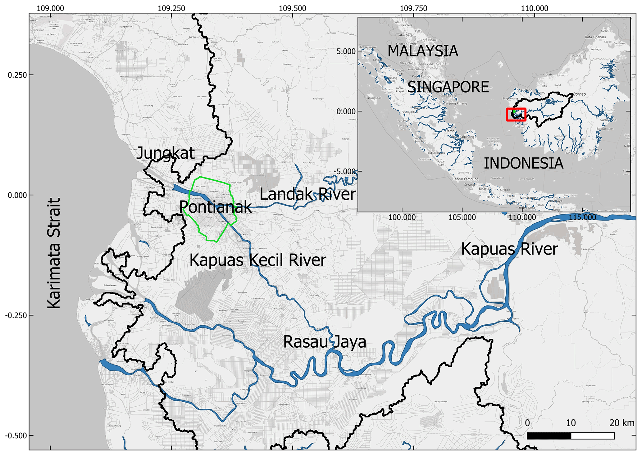
Figure 1The region of interest (ROI), where the green enclosed perimeter represents the city of Pontianak. The solid black line represents the Kapuas River watershed in the inset map, and the blue lines represent waterbodies. The background map is retrieved from Planet dump (retrieved from https://planet.osm.org, last access: 3 April 2021, 2020). © OpenStreetMap contributors, 2017. Distributed under the Open Data Commons Open Database License (ODbL) v1.0.

Figure 2Kapuas water catchment area (upper left), digital elevation map (DEM) (upper right) retrieved from SRTM (Farr et al., 2007), land cover maps (lower left) retrieved from CGLOPS1 (Buchhorn et al., 2020), and soil type maps (lower right) retrieved from FAO (Sanchez et al., 2009) for the Kapuas River catchment area.
2.1 Study area
The Kapuas River is the longest inland river in Indonesia (Goltenboth et al., 2006). The basin is located in the western part of the Borneo Island (Fig. 1). The water catchment area spreads over about 93 000 km2 (about 12.5 % of the Borneo Island area, Fig. 1), with approximately 66.7 % of it consisting of forests (Wahyu et al., 2010). The upstream topography comprises hills covered mainly by Acrisol soils (Fig. 2), and the downstream consists of plains with more heterogeneous soil types (Fig. 2), such as Humic Gleysols (derived from grass or forest vegetation) and Dystric Fluvisols (young soil in alluvial deposits). For the local communities the river is vital as a source of fresh water and a transportation system.
In the last decades, palm oil cultivation and forest fires expanded massively in the Kapuas water catchment (Semedi, 2014; Jadmiko et al., 2017). These circumstances changed the Kapuas hydrological regime and triggered more intense flooding in the river's floodplains. Combined with global sea level rise, these phenomena could lead to more intense and severe flood events, particularly in the river delta.
The delta of the Kapuas River is still mostly natural, with no dams, dikes, or groins on its downstream. Therefore, the hydrodynamics of the river significantly influence the flood occurrences in the delta. The most populated area over the delta is Pontianak, a city located in the Kapuas Kecil – the middle stream of the second-largest branch of the Kapuas River.
As a tidal river, the tidal regime within the Kapuas River delta is mixed but mainly diurnal (Kästner, 2019). The dominant tidal constituent is K1, O1, P1, M2, and S2 (Pauta, 2018). The average tidal amplitude within the delta is set in a microtidal regime, with a mean spring range of 1.45 m at its river mouth (Kästner, 2019).
2.2 Hydrodynamic model description
To simulate hydrodynamics within the Kapuas River delta, we use the multi-scale hydrodynamic model SLIM 2D (Lambrechts et al., 2008; Gourgue et al., 2009; Remacle and Lambrechts, 2016). SLIM 2D is an unstructured-mesh hydrodynamic model (https://www.slim-ocean.be/). The model can simulate hydrodynamic processes along the land–sea continuum, from the river to the ocean (Vallaeys et al., 2018, 2021; Frys et al., 2020; Le et al., 2020b). We simulate compound flooding events based on the water level dynamics for different forcing scenarios using the model. The model solves the 2D shallow water equations (SWE).
H is the water column height, ∇ is the horizontal gradient operator, is the horizontal transport, R is the rainfall, t is the time, is the depth-averaged horizontal velocity, f is the Coriolis parameter, ez is the vertical unit vector pointing upward, υ is the horizontal eddy viscosity, α is a constant to define dry elements (α=0) and wet elements (α=1) (Le et al., 2020a), h is the bathymetry, g=9.81 m s−2 is the gravitational acceleration, Cd is the bulk drag coefficient, τwind is the wind stress, and ∇Patm is the atmospheric pressure gradient.
2.3 Metrics for model performance evaluation
We use the Nash–Sutcliffe efficiency (NSE) measure to evaluate the models' performance. The NSE is used to assess the performance of the ML models in producing the predicted water level. A perfect model corresponds to NSE = 1, while a model that has the same predictive skill as the mean of the observed data is represented by NSE = 0. Meanwhile, NSE < 0 implies that the mean value of observed data predicts better than the model. The closer the NSE value is to 1, the better the predictive skill of the model. The NSE coefficient is calculated as follows:
where represents the water level model at time t, represents the observed water level at the same time, and is the mean of the observed water level.
Root mean square errors (RMSEs) of peaks between predicted water level and observation during the flood events are also used as an additional performance indicator. The RMSE is used to represent the model's ability to predict flood events. The RMSE between the model outputs and the observations is calculated by
where xi is the water level as the model's output at the ith peak, and yi is the observed water level at the same time. The number of the total peak data is N.
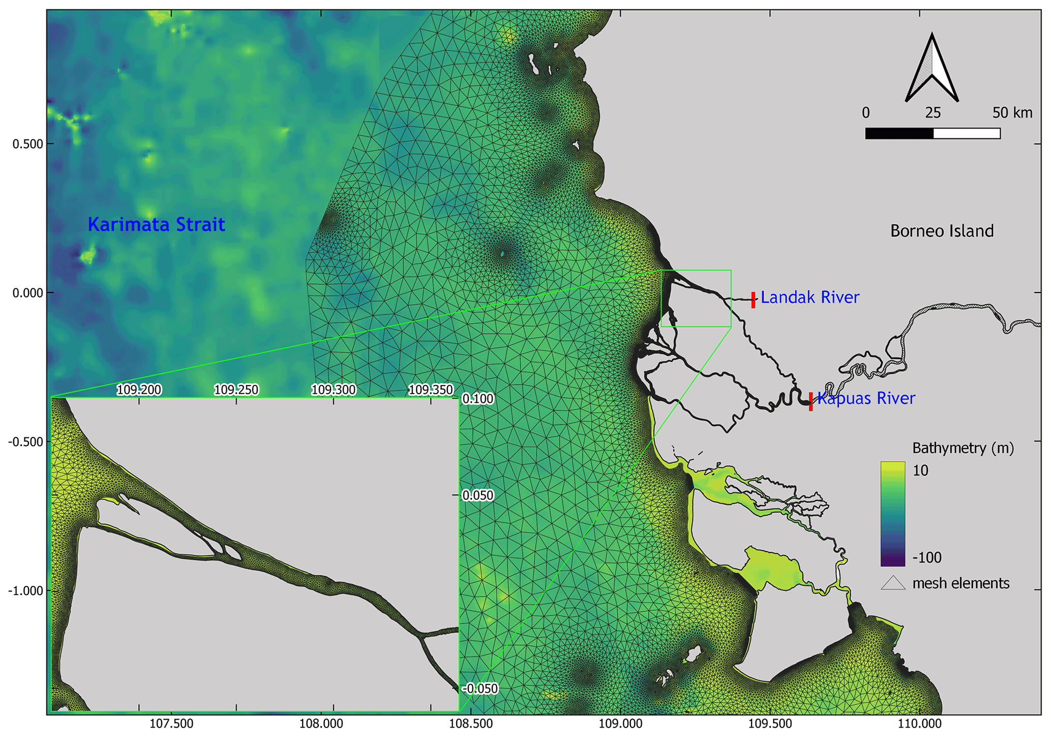
Figure 3The hydrodynamic model domain is discretized with an unstructured mesh with its resolution set to 50 m along the riverbanks, 400 m along the coast near the estuary, 1 km over the rest of the coastline, and 5 km offshore. The bathymetry of the model domain ranges from ∼ 100 m depth offshore to 1 m in the river mouth.
2.4 Hydrodynamic model setup and calibration
In order to run the hydrodynamic model, we defined a computational domain that covers both the river and ocean parts. Next, we generated an unstructured mesh to cover the domain, with a resolution of 50 m over the riverbanks, 400 m over the coast near the river mouth, 1 km over the rest of the coastline, and 5 km offshore (Fig. 3). The multi-scale mesh was generated using an algorithm developed by Remacle and Lambrechts (2018). We then set the bathymetry constructed from two datasets: (i) the river and estuary bathymetry maps, obtained from the Indonesian Navy (Kästner, 2019), and (ii) the Karimata Strait bathymetry, obtained from BATimetri NASional (BATNAS, 2021). Furthermore, we set the bulk bottom drag coefficients, which are 2.5 × 10⁻³ over the ocean (corresponding to a sandy seabed) and 1.9 × 10⁻² over the riverbed (Kästner et al., 2018). Lastly, we imposed the rainfall, as observed by the Pontianak Maritime Meteorological Station (PMMS).
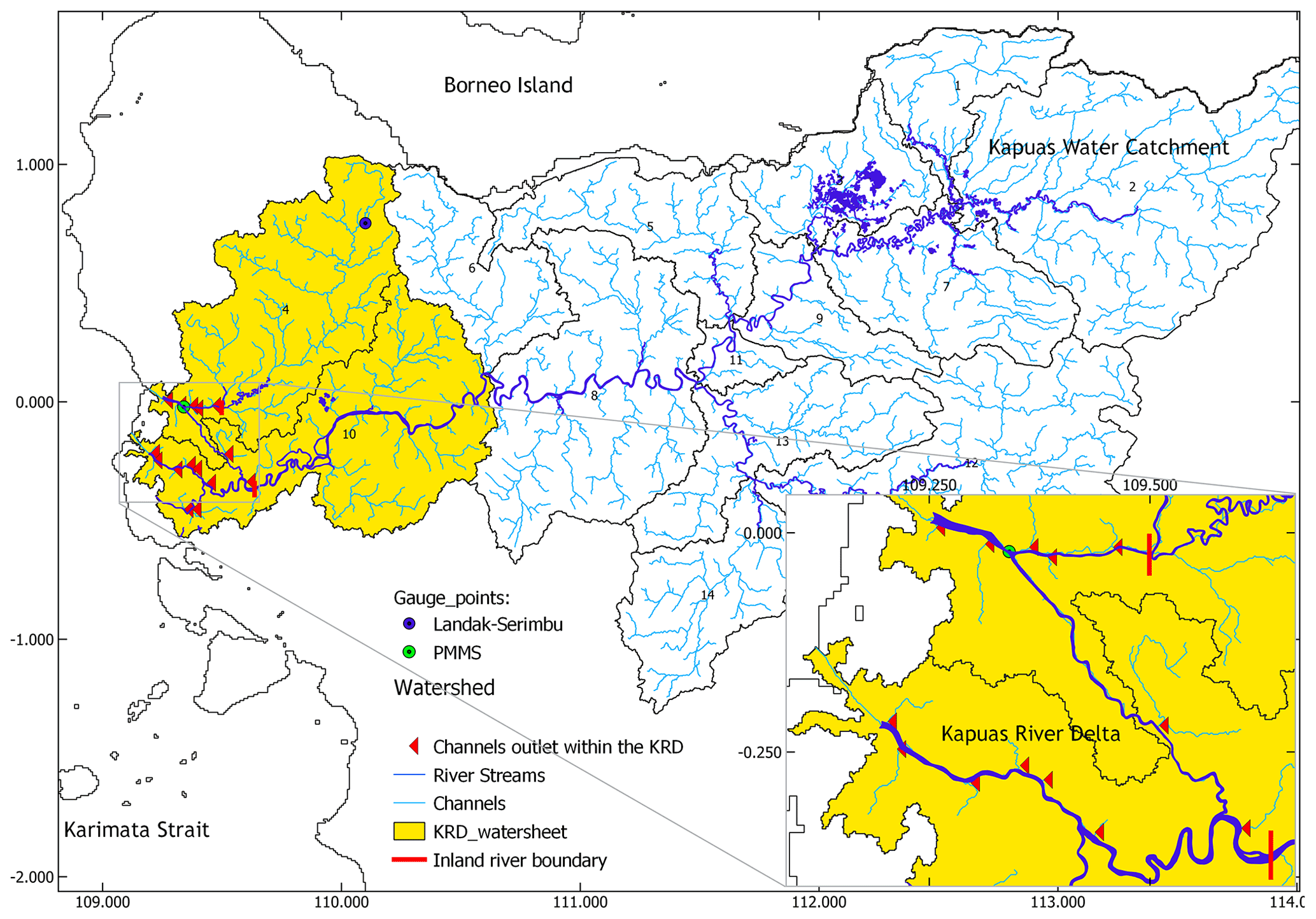
Figure 4The Kapuas River watershed and its sub-basins. Since the discharges of the Kapuas River are retrieved at the middle stream, only two sub-basins are considered for the SWAT+ model (yellow area). The runoffs (channel outlets of the SWAT+ model that enter the river stream within the KRD) are set as inlets for the hydrodynamic model domain.
The hydrodynamic model simulation is forced by wind and atmospheric pressure from ECMWF (Hersbach et al., 2020), and tides from TPXO (Egbert and Erofeeva, 2002). As upstream boundary conditions, we imposed discharge from the Kapuas and Landak rivers and the discharge data were retrieved from the Global Flood Monitoring System (GFMS) (Wu et al., 2014) at about 70 and 40 km from the river mouth, respectively (Fig. 4). Since the GFMS calculates the flow using Integrated Multi-Satellite Retrievals for GPM (IMERG) precipitation information as input, the coastal processes do not affect the model output (predicted river flow).
We also imposed runoff, obtained by converting rainfall over the Kapuas Kecil River catchment area as an inlet water flux at 15 channels entering the domain (Fig. 4). The runoff of every channel was calculated from rainfall data using SWAT+ (Bieger et al., 2017), which considered the pressure, humidity, and other weather parameter input. Here, we use one-way coupling, where the SWAT+ model runs first and independently. The SWAT+ model only produces the flow of channels that enter the river stream within the Kapuas River delta. Then, we used these channel outlets as boundary conditions for the SLIM 2D model. Unfortunately, during the tuning of the SWAT+ model, the correlation between the model's output (runoff) and the observation data is still low (Pearson correlation coefficient =0.32). However, we decided to use the output as the channels' inlet boundary condition in the hydrodynamic model because the channel runoff volume is much less than the river discharge. Therefore, we assumed that it does not significantly affect the hydrodynamics of the river.
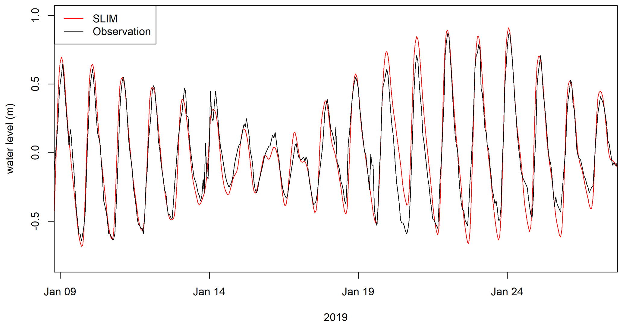
Figure 5The SLIM 2D model's output validation with respect to observational data at Pontianak in January 2019, with NSE =0.87 and RMSE =0.12 m, indicating that the model has satisfactory performance.
To evaluate the SLIM 2D model's performance, we ran a simulation for January 2019 and compared the simulated water elevation with the observations in Pontianak. The model errors correspond to an NSE of 0.87 and an RMSE of 0.12 m (Fig. 5). This RMSE is deemed sufficiently small to consider model outputs as a good proxy for the real system (Moriasi et al., 2015).
Table 1Scenarios used to force the process-based hydrodynamic model.
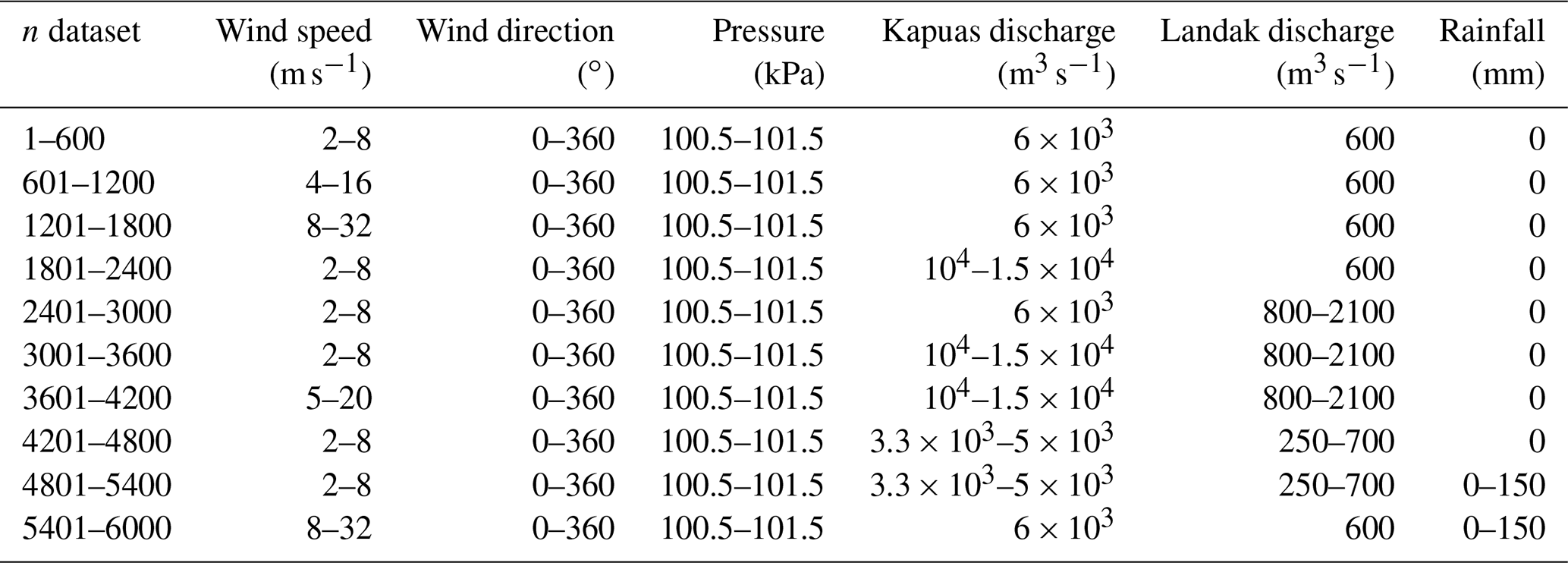
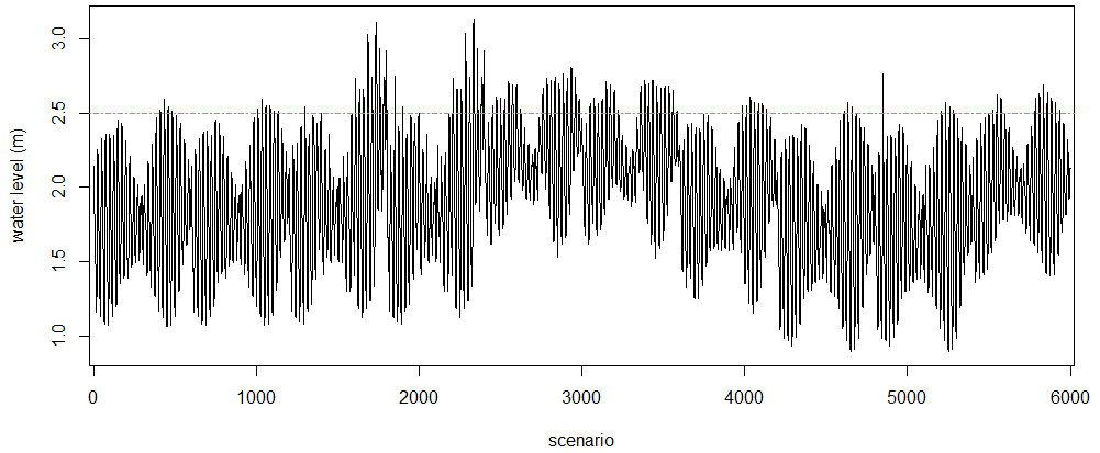
Figure 6The Kapuas Kecil River's water level in Pontianak, obtained from the hydrodynamic model. The green dashed line is the threshold above which the water starts to overflow the riverbanks in Pontianak.
We simulated the hydrodynamics with different oceanic, atmospheric, and river forcings to forecast flood events based on the water levels in Pontianak. Based on the PMMS report, the city is flooded when the water level exceeds 2.5 m. We, therefore, set this value as the threshold of a flood event. We ran the hydrodynamic model for 10 months and extracted the output hourly to produce the scenarios (see Table 1). Then, we selected 6000 sample points of the predicted water levels at Pontianak with their associated input dataset using a random sampling technique. We merged the data as a single dataset to train the ML model, encompassing all possible flood events resulting from the combination of the external forcings. The dataset shows that several floods occurred within the simulations, indicated by sample points with water elevations greater than 2.5 m (Fig. 6).
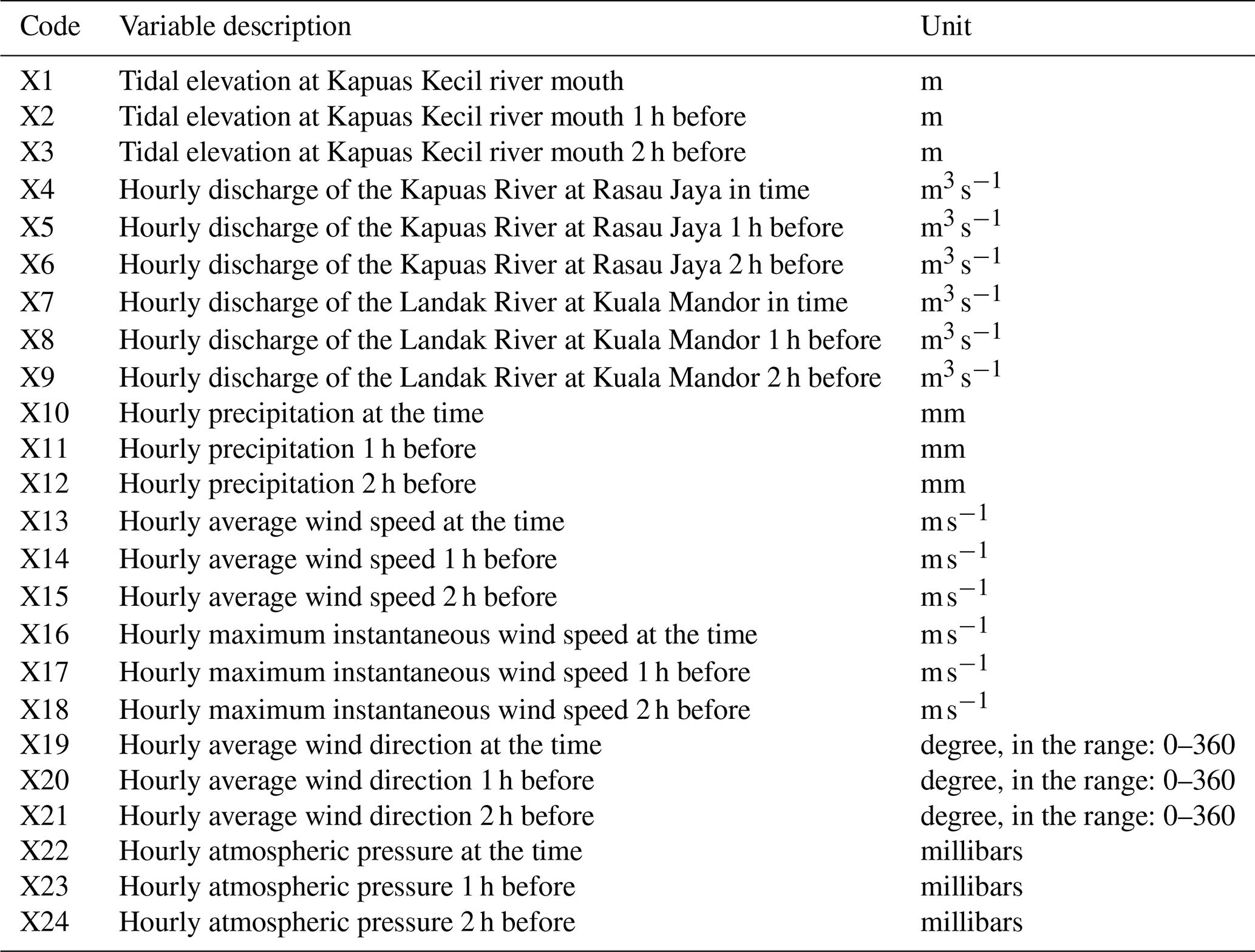
Table 2The variables which are used as the predictors in this study.
2.5 Machine learning (ML) model
2.5.1 Dependent and predictor variables
To develop the ML models, we used the river water level at Pontianak as the dependent variable. Then, we considered atmospheric, oceanic, and riverine variables as predictors of the water level in the city. Atmospheric variables include average and maximum wind speed, wind direction, precipitation, and average atmospheric pressure. Oceanic variables cover tides at the river mouth, and the riverine variables consist of the Kapuas River and the Landak River discharges. To evaluate the impact of each predictor before the flood event, we imposed the prior state (1 and 2 h before) of these parameters (see Table 2). The datasets were recorded hourly and combined with the SLIM 2D output (used in the training and testing phases) and the observational data (used in the implementation phase).

Figure 7Mutual information (MI) of all predictor variables to hourly water level dynamics in 3 months of observational data.
Mutual information (MI), a statistic tool that can measure the degree of relatedness between variables in a dataset, was implemented to evaluate the relation between each predictor and the dependent variable (Fig. 7). The greater the MI value between two variables, the stronger the relatedness, regardless of how nonlinear its dependency is (Kinney and Atwal, 2014). The MI between two variables (X and Y) is obtained from Choi et al. (2020):
where p(xy) is the joint probability distribution.
All predictors considered in the ML model have an MI coefficient greater than zero, which means all predictor variables impact the river water level in Pontianak (Fig. 7). The relationship between these predictors and the water level could be linear or nonlinear (as shown by MI capturing both relation types). Here, we found that the tidal elevations in the river mouth (X1, X2, and X3) have the most decisive impact on the river water level in the city (MI > 0.5), while tidal elevation observed 1 h before (X2) is the strongest one. Next, the wind speed (maximum and average), the discharges (from both the Kapuas and the Landak rivers), and the pressure have a moderate relatedness. In contrast, the wind direction and the rainfall only have weak relatedness (MI < 0.1). This means that both parameters have no significant impact.
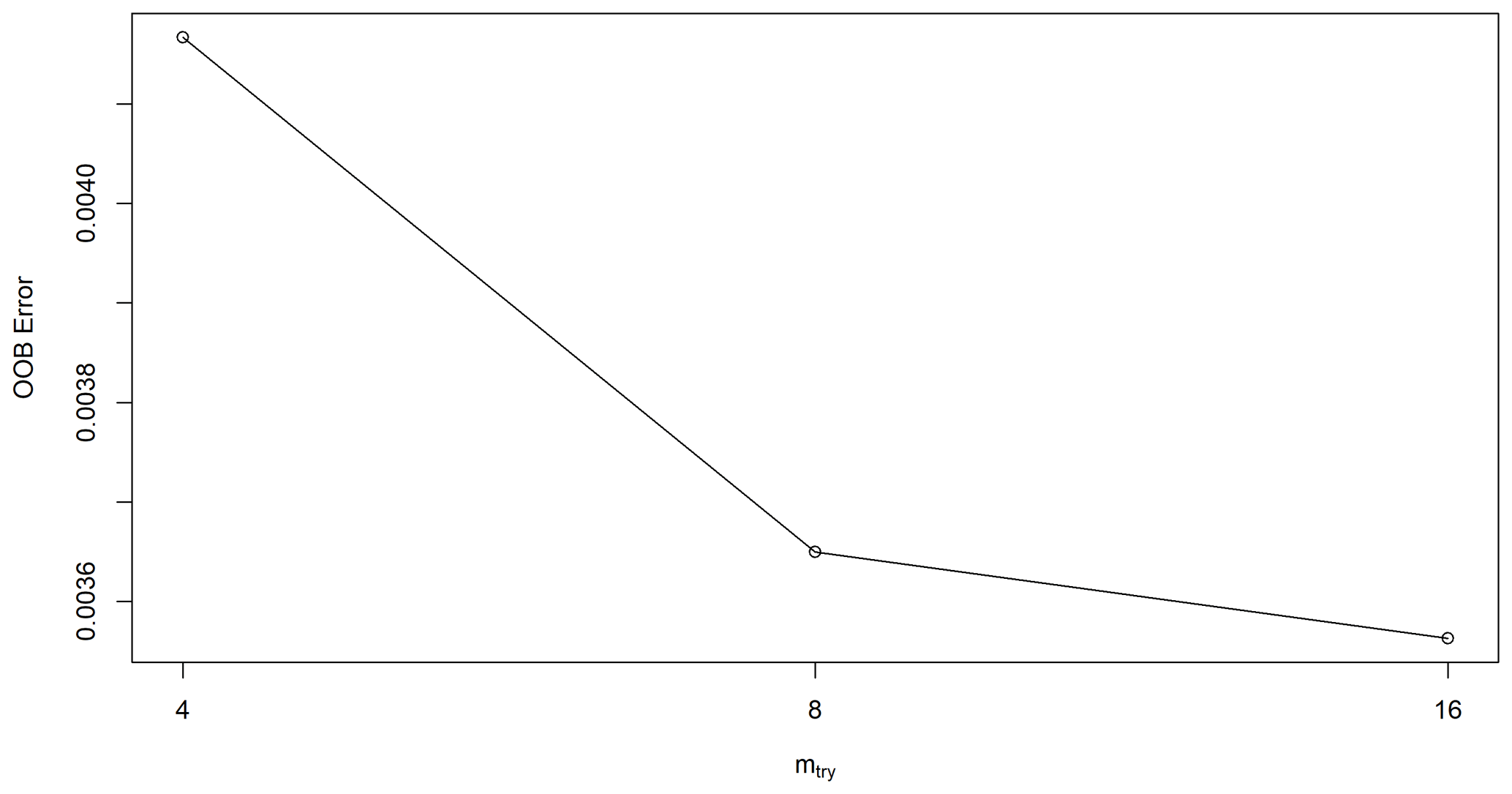
Figure 8Tuned randomForest algorithm for the optimal number of variables randomly sampled as candidates at each split (mtry) parameter.
2.5.2 Machine learning (ML) algorithm
Here, we consider three different machine learning algorithms, i.e., random forest (RF), multiple linear regression (MLR), and support vector machine (SVM). The RF is a supervised learning algorithm that operates by constructing many decision trees during the training (Breiman, 2001). The algorithm can be implemented for classification or regression. The model aggregates its multiple decision tree outcomes to generate the ultimate output, which is called the sub-sample outcomes (Han et al., 2012). The technique was enhanced by combining bootstrap with its aggregating processes (Breiman, 2001). Using this strategy, the algorithm became an effective tool for classification and regression. In this study, the RF algorithm was obtained from the R randomForest library (Liaw and Wiener, 2002). To obtain the optimal parameter for RF, we first tune the algorithm by searching for the optimal value of the number of variables randomly sampled as candidates at each split (mtry). As a result, the optimal number is 16 (Fig. 8).
The MLR is a statistical technique that uses several explanatory variables to predict the outcome of a response variable (James et al., 2013). This method fits the linear relationship between input features and the target (observed data) using the least-squared approach. In the least-squared approach, the best relationship model will be obtained by minimizing the sum of the squared distance between the calculated values (as model outputs) and the target values (James et al., 2013). This algorithm is the most straightforward approach in ML models and is generally used as the baseline method. The MLR algorithm implemented in this study was obtained from the R RWeka library (Hornik et al., 2008).
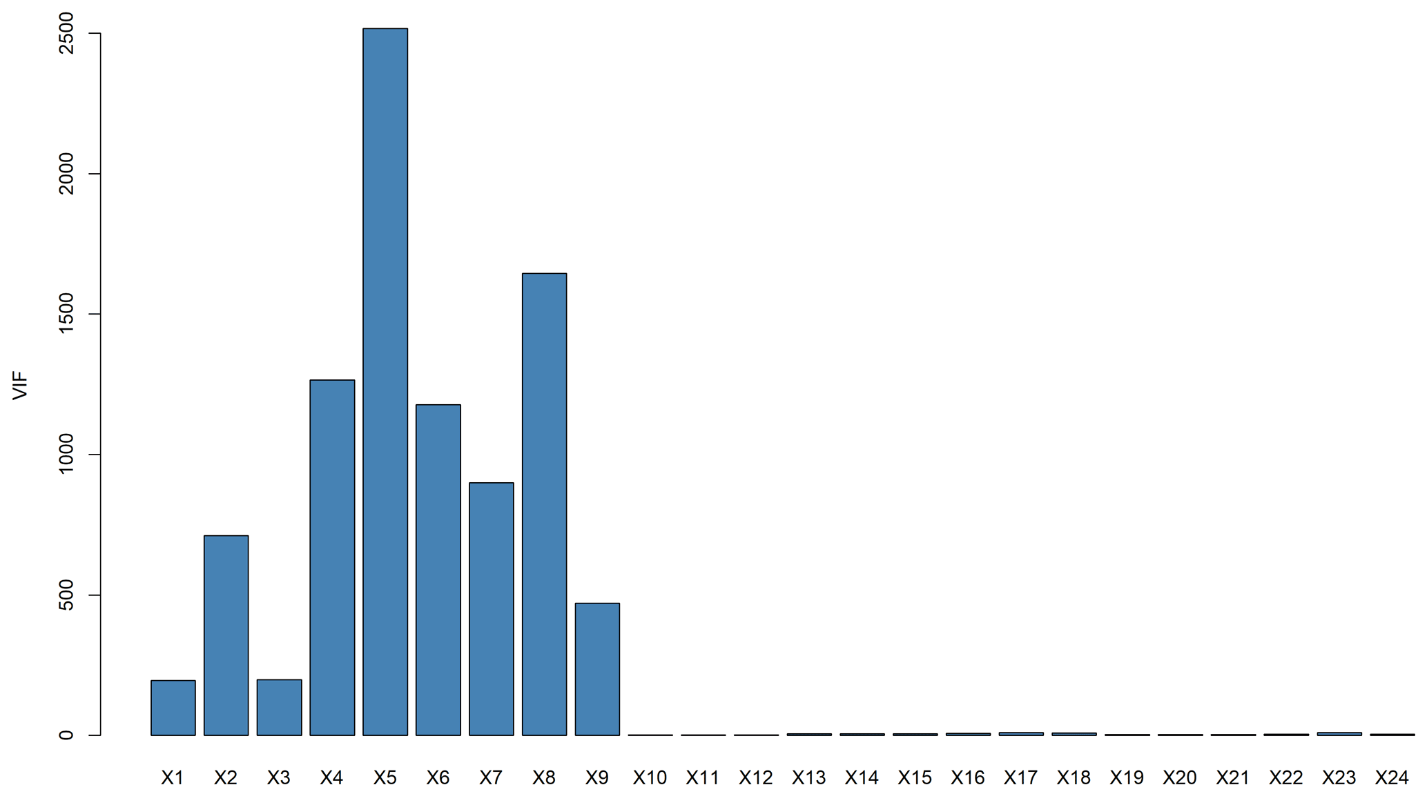
Figure 9Variance inflation factor (VIF) values of all predictor's variables in 3 months of observational data.
To obtain the best performance of the MLR algorithm, we did a statistical analysis to evaluate the multicollinearity among the predictor variables using the Variance inflation factor (VIF). Since multicollinearity negatively affects the performance of the MLR model, VIF can help reduce the number of predictors (Alipour et al., 2020). Here, we found that some variables have a VIF more significant than 5, which indicates a potentially severe correlation between these variables in the model (Fig. 9). Therefore, combined with the output of the MI analysis, we removed some variables which have low MI and a high VIF.
The SVM is a supervised ML algorithm based on statistical learning frameworks (Gholami and Fakhari, 2017). This method is robust for modeling a complex nonlinear relationship. The kernel function transforms the input features into a high-dimensional space to tackle the complexity. This transforms the nonlinear relationship of input features into linear ones. Finally, linear regression is carried out to obtain the ultimate output. Compared to the other algorithms, SVM needs less computational resources because it can be trained by only a few features (Gholami and Fakhari, 2017). Previously, SVM was only implemented for classification purposes, but it has also been implemented for regression purposes after some enhancement. The SVM algorithm implemented in this study was obtained from the R MARSSVRhybrid library (MARSSVRhybrid: MARS SVR Hybrid; Das et al., 2021).
Since the kernel function is critical in SVM, we tuned the SVM algorithm to obtain good results by selecting the most appropriate kernel parameter. We tested four kernels, i.e., linear, polynomial, radial basis, and sigmoid, as the candidates. We found that the radial basis kernel performed the best for the SVM algorithm.
2.6 Model limitations
During the development process, we encountered potential errors that could be highlighted as model limitations. Firstly, we assumed that the channel runoff volume would not affect the hydrodynamics of the river due to its small volume compared to the riverine volume. The average daily discharge of the Kapuas and Landak rivers during the simulation is about 4137 and 406 m3 s−1, respectively. At the same time, the total daily runoff of all channels that enter the hydrodynamic model domain in the Kapuas River delta is about 32 m3 s−1. The runoff contributes only about 0.7 % of the total inlets in the hydrodynamic simulations; therefore, we assumed it is insignificant.
Secondly, we assumed that all the possible compound flood scenarios would occur within 10 months. Since we had already set some extreme values in the predictor parameters during the time, we assumed that all possible causes that drive compound flooding in the domain are represented. However, this assumption may not be accurate.
Next, we only imposed the runoffs as inlets on the riverbanks in the hydrodynamic model domain. Hence, the model did not capture the hydrodynamic processes in the channels within the city. This means that the inundation processes in Pontianak were still not well represented. The model still lacks drainage systems for the urban region.
Moreover, the accuracy of the ML model depends on the hydrodynamic model's accuracy. The more accurate the hydrodynamic model in predicting observational floods, the better the ML model will perform. Therefore, we need to tune the hydrodynamic model as accurately as possible.
Furthermore, since the rainfall impact on river water level is minor compared to other parameters, the model could not optimally capture urban flooding due to excessive rainfall. Based on the field observation, the city is shortly inundated if rain falls excessively for a few hours. This inundation could be due to the poor quality of the urban drainage system. Unfortunately, this phenomenon is not directly captured by the water level observation located within the river. The increase in the river water level due to the heavy rain is minor.
Lastly, the model relies on the predicted input parameters such as weather parameters and river discharges to predict the future water level. Consequently, the more biased the predictors, the higher the uncertainty in the water level prediction. Therefore, observational data as input parameters are needed to reduce the uncertainty and create a more robust model.
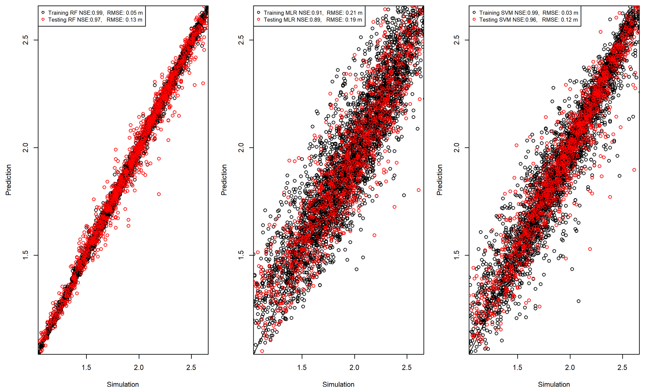
All NSE coefficients were greater than 0.8 in both the training and testing phases, which means that all algorithms perform very well. The most accurate algorithm is RF, followed by SVM and MLR (Fig. 10). As such, we know that all the tested ML algorithms are promising and need to be evaluated in the implementation phase using observational data.

Figure 11Comparison of predicted hourly water levels models and measured hourly water levels for the implementation phase on: (a) December 2018, (b) January 2020, and (c) January 2021
Therefore, we implemented the ML models on the selected observational data, which were obtained during the high discharge season for 3 months in 3 years when inundations occurred (December 2018, January 2020, January 2021). Figure 11 shows each proposed algorithm's predicted water levels compared to the observational data. Subsequently, the accuracy of models to predict flooding events, marked by points in Fig. 11, is evaluated.
Even though all algorithms performed very well during the training and testing phases, the performances differed during the implementation phase (Table 3). However, RF showed high accuracy in the three different implementation phases. From the three different observational datasets, RF's NSE values range from 0.61 to 0.72, which is a good performance.
Table 3Performance of the three machine learning (ML) algorithms in implementation phase.
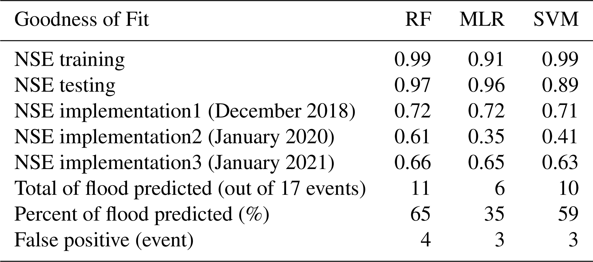
While the MLR algorithm succeeded in the training and testing phases, it only succeeded in the first and third implementation phases, with NSE of 0.72 and 0.65, respectively. The model was less successful in the second implementation phase, with NSE hitting only 0.35 for this implementation dataset.
Next, the SVM algorithm's performance is similar to that of the MLR algorithm. It succeeded in the training and testing phases but only succeeded in the first and third implementation phases, with NSE reaching 0.71 and 0.63, respectively. However, it failed in the second implementation dataset, with an NSE of only 0.41, which is slightly better than MLR.
Regarding the prediction of flood events, the RF algorithm also performed better than the other algorithms. It could predict 11 out of 17 events (65 % accuracy). On the other hand, MLR and SVM could only predict 6 and 10 events (35 % and 59 % accuracy), respectively. Therefore, we know that RF is the most accurate ML algorithm to predict floods for our test case.
Unfortunately, these three algorithms also predicted false-positive events, i.e., flood events that never occurred during implementation (Table 3). While RF predicted four false events, MLR and SVM predicted three false events. This false event prediction is the shortcoming of the algorithm, which should be addressed in future studies.
The two main issues that have been tackled in this study are data scarcity and low computational resources for building flood forecasting models based on the water level dynamics in developing countries (Brocca et al., 2020; Singh et al., 2021). Here we showed that using an approach that combines hydrodynamic and ML models is promising for obtaining a reliable and robust water level model. We succeeded in building and evaluating ML models trained by the hydrodynamic model output; hence, they did not require extensive observational data in their training phase and did not need high computational costs in their implementation. Therefore, the proposed model is reliable for areas where observational data are scarce and computational resources are limited.
Since the proposed model can accurately forecast water levels, local water management agencies can rely on the model outputs for flood forecasting. Since ML does not require high computational resources, limited computational resources will not hinder the assessment and mitigation of compound flooding hazards. Using the model, agencies can re-assess their compound flood hazards and predict future events. Moreover, once they have more observation data, they can use it to re-adjust the proposed model or build a more robust one (Muñoz et al., 2021).
Next, we found that the RF algorithm is the best ML algorithm to predict water level as a proxy for compound flooding in the area of interest. In general, the performances of all tested ML algorithms for water level prediction are reasonable and acceptable. However, considering the NSE values in all implementation phases, the number of flood events that are accurately predicted, and how close the predicted water level is during the events, it could be concluded that RF performs better than other algorithms. The superiority of the RF algorithm in predicting water levels has also been shown in previous studies in the Upo Wetland (Choi et al., 2020) and the Poyang Lake (Li et al., 2016). Therefore, we proposed a ML model with the RF algorithm as the most appropriate model for the study area.
In addition, we found that the tidal elevation measured 1 h prior at the river mouth is the main parameter controlling the river water level in Pontianak. Even though the city is located 20 km from the river mouth, the tidal dynamics still strongly affect the river water level in the city. This result confirms previous studies, revealing that the tide propagation on the Kapuas River dominantly controls the river water level up to 30 km upstream (BGD – Modeling interactions between tides, storm surges, and river discharges in the Kapuas River delta, 2021), and still impacts up to 285 km from the river mouth (Kästner et al., 2019).
Overall, our integrated approach can provide a model to predict compound flooding driven by the interaction of tide, wind surge from the ocean, and high discharge from the river upstream. Regarding the limitation of the chosen indicator's capability to capture flood events, we will look for more data and indicators to enhance the model capability in future studies. Moreover, we will reduce the number of predictors to minimize the model output's uncertainty. We will also evaluate mean sea level rise due to climate change to broaden the model implementation and create better flood mitigation.
This study shows that an integrated approach between the hydrodynamic and the ML models successfully overcomes modeling river water level and predicting compound flooding hazards in a data-scarce environment with limited computational resources. Therefore, the approach is suitable for local water management agencies in developing countries that are faced with these issues. However, the accuracy of the ML model depends on the accuracy of the hydrodynamic model. If the hydrodynamic model is inaccurate in predicting real-life floods, the ML model's accuracy will also be lower. Besides, it has not yet optimally captured the urban flooding due to excessive rainfall. The consideration of more indicators representing this kind of flooding is essential to enhance the model's capability in future. Regarding the implementation in Pontianak, we found that the ML model with the RF algorithm has the most accurate output compared to the other algorithms. In addition, the tidal elevation, measured 1 h prior, is the main predictor for water level modeling in the study area.
The R code used in this study can be accessed at https://doi.org/10.5281/zenodo.6795949 (Sampurno, 2022).
The data used in this study is available at https://doi.org/10.5281/zenodo.6795963 (Sampurno and Ardianto, 2022). The water level data were collected by Pontianak Maritime Meteorological Station (PMMS), Indonesia. To use the data, please cite this article and the official web page of PMMS: https://maritim.kalbar.bmkg.go.id/ (last access: 20 November 2021; PMMS, 2021).
JS, VV, and EH conceptualized the research; JS and RA curated the data; JS, VV, and EH analyzed the data; JS wrote the manuscript draft; JS and EH reviewed and edited the manuscript.
The contact author has declared that none of the authors has any competing interests.
Publisher's note: Copernicus Publications remains neutral with regard to jurisdictional claims in published maps and institutional affiliations.
Computational resources have been provided by the supercomputing facilities of the Université catholique de Louvain (CISM/UCL) and the Consortium des Équipements de Calcul Intensif en Fédération Wallonie Bruxelles (CÉCI) funded by the Fond de la Recherche Scientifique de Belgique (F.R.S.-FNRS) under convention 2.5020.11 and by the Walloon Region.
This research has been supported by the Indonesia Endowment Fund for Education – Lembaga Pengelola Dana Pendidikan (LPDP; grant no. 201712220212183).
This paper was edited by Stefano Pierini and reviewed by two anonymous referees.
Alipour, A., Ahmadalipour, A., Abbaszadeh, P., and Moradkhani, H.: Leveraging machine learning for predicting flash flood damage in the Southeast US, Environ. Res. Lett., 15, 024011, https://doi.org/10.1088/1748-9326/AB6EDD, 2020.
Assem, H., Ghariba, S., Makrai, G., Johnston, P., Gill, L., and Pilla, F.: Urban Water Flow and Water Level Prediction Based on Deep Learning, in: Machine Learning and Knowledge Discovery in Databases, ECML PKDD 2017, Lecture Notes in Computer Science, Springer, Cham, 10536, 317–329, https://doi.org/10.1007/978-3-319-71273-4_26, 2017.
BATimetri NASional: https://tanahair.indonesia.go.id/demnas/#/batnas, last access: 14 July 2021.
Bevacqua, E., Maraun, D., Vousdoukas, M. I., Voukouvalas, E., Vrac, M., Mentaschi, L., and Widmann, M.: Higher probability of compound flooding from precipitation and storm surge in Europe under anthropogenic climate change, Sci. Adv., 5, eaaw5531, https://doi.org/10.1126/sciadv.aaw5531, 2019.
Bhaskaran, P. K., Gayathri, R., Murty, P. L. N., Bonthu, S. R., and Sen, D.: A numerical study of coastal inundation and its validation for Thane cyclone in the Bay of Bengal, Coast. Eng., 83, 108–118, https://doi.org/10.1016/J.COASTALENG.2013.10.005, 2014.
Bieger, K., Arnold, J. G., Rathjens, H., White, M. J., Bosch, D. D., Allen, P. M., Volk, M., and Srinivasan, R.: Introduction to SWAT+, a Completely Restructured Version of the Soil and Water Assessment Tool, J. Am. Water Resour. Assoc., 53, 115–130, https://doi.org/10.1111/1752-1688.12482, 2017.
Bilskie, M. V. and Hagen, S. C.: Defining Flood Zone Transitions in Low-Gradient Coastal Regions, Geophys. Res. Lett., 45, 2761–2770, https://doi.org/10.1002/2018GL077524, 2018.
Breiman, L.: Random forests, Mach. Learn., 45, 5–32, https://doi.org/10.1023/A:1010933404324, 2001.
Brocca, L., Massari, C., Pellarin, T., Filippucci, P., Ciabatta, L., Camici, S., Kerr, Y. H., and Fernández-Prieto, D.: River flow prediction in data scarce regions: soil moisture integrated satellite rainfall products outperform rain gauge observations in West Africa, Sci. Rep., 101, 1–14, https://doi.org/10.1038/s41598-020-69343-x, 2020.
Buchhorn, M., Lesiv, M., Tsendbazar, N.-E., Herold, M., Bertels, L., and Smets, B.: Copernicus Global Land Cover Layers – Collection 2, Remote Sens.-Basel, 12, 1044, https://doi.org/10.3390/RS12061044, 2020.
Chan, N. W.: Impacts of Disasters and Disaster Risk Management in Malaysia: The Case of Floods, in: Resilience and Recovery in Asian Disasters, edited by: Aldrich, D., Oum, S., and Sawada, Y., Springer, Tokyo, 18, 239–265, https://doi.org/10.1007/978-4-431-55022-8_12, 2015.
Chen, J. H. and Asch, S. M.: Machine Learning and Prediction in Medicine – Beyond the Peak of Inflated Expectations, N. Engl. J. Med., 376, 2507, https://doi.org/10.1056/NEJMP1702071, 2017.
Choi, C., Kim, J., Han, H., Han, D., and Kim, H. S.: Development of Water Level Prediction Models Using Machine Learning in Wetlands: A Case Study of Upo Wetland in South Korea, Water, 12, 93, https://doi.org/10.3390/W12010093, 2020.
Comer, J., Olbert, A. I., Nash, S., and Hartnett, M.: Development of high-resolution multi-scale modelling system for simulation of coastal-fluvial urban flooding, Nat. Hazards Earth Syst. Sci., 17, 205–224, https://doi.org/10.5194/nhess-17-205-2017, 2017.
Costabile, P. and Macchione, F.: Enhancing river model set-up for 2-D dynamic flood modelling, Environ. Model. Softw., 67, 89–107, https://doi.org/10.1016/J.ENVSOFT.2015.01.009, 2015.
Costabile, P., Costanzo, C., and Macchione, F.: A storm event watershed model for surface runoff based on 2D fully dynamic wave equations, Hydrol. Process., 27, 554–569, https://doi.org/10.1002/HYP.9237, 2013.
Couasnon, A., Eilander, D., Muis, S., Veldkamp, T. I. E., Haigh, I. D., Wahl, T., Winsemius, H. C., and Ward, P. J.: Measuring compound flood potential from river discharge and storm surge extremes at the global scale, Nat. Hazards Earth Syst. Sci., 20, 489–504, https://doi.org/10.5194/nhess-20-489-2020, 2020.
Das, P., Lama, A., and Jha, G.: MARSSVRhybrid: MARS SVR Hybrid, https://cran.r-project.org/web/packages/MARSSVRhybrid/index.html, last access: 23 September 2021.
Egbert, G. D. and Erofeeva, S. Y.: Efficient inverse modeling of barotropic ocean tides, J. Atmos. Ocean. Tech., 19, 183–204, 2002.
El Naqa, I., Ruan, D., Valdes, G., Dekker, A., McNutt, T., Ge, Y., Wu, Q. J., Oh, J. H., Thor, M., Smith, W., Rao, A., Fuller, C., Xiao, Y., Manion, F., Schipper, M., Mayo, C., Moran, J. M., and Ten Haken, R.: Machine learning and modeling: Data, validation, communication challenges, Med. Phys., 45, e834–e840, https://doi.org/10.1002/MP.12811, 2018.
Farr, T. G., Rosen, P. A., Caro, E., Crippen, R., Duren, R., Hensley, S., Kobrick, M., Paller, M., Rodriguez, E., Roth, L., Seal, D., Shaffer, S., Shimada, J., Umland, J., Werner, M., Oskin, M., Burbank, D., and Alsdorf, D. E.: The Shuttle Radar Topography Mission, Rev. Geophys., 45, 2004, https://doi.org/10.1029/2005RG000183, 2007.
Frys, C., Saint-Amand, A., Le Hénaff, M., Figueiredo, J., Kuba, A., Walker, B., Lambrechts, J., Vallaeys, V., Vincent, D., and Hanert, E.: Fine-Scale Coral Connectivity Pathways in the Florida Reef Tract: Implications for Conservation and Restoration, Front. Mar. Sci., 7, 312, https://doi.org/10.3389/FMARS.2020.00312, 2020.
Ghanbari, M., Arabi, M., Kao, S. C., Obeysekera, J., and Sweet, W.: Climate Change and Changes in Compound Coastal-Riverine Flooding Hazard Along the U. S. Coasts, Earths Future, 9, e2021EF002055, https://doi.org/10.1029/2021EF002055, 2021.
Gholami, R. and Fakhari, N.: Support Vector Machine: Principles, Parameters, and Applications, in: Handbook of Neural Computation, edited by: Samui, P., Sekhar, S., and Balas, V. E., Elsevier Inc., Academic Press, London, UK, 515–535, https://doi.org/10.1016/B978-0-12-811318-9.00027-2, 2017.
Goltenboth, F., Timotius, K. H., Milan, P. P., and Margraf, J.: Ecology of insular Southeast Asia: the Indonesian archipelago, Elsevier B. V., https://doi.org/10.1016/B978-0-444-52739-4.X5000-1, 2006.
Gori, A., Lin, N., Xi, D., and Emanuel, K.: Tropical cyclone climatology change greatly exacerbates US extreme rainfall–surge hazard, Nat. Clim. Change, 122, 171–178, https://doi.org/10.1038/s41558-021-01272-7, 2022.
Gourgue, O., Comblen, R., Lambrechts, J., Kärnä, T., Legat, V., and Deleersnijder, E.: A flux-limiting wetting–drying method for finite-element shallow-water models, with application to the Scheldt Estuary, Adv. Water Resour., 32, 1726–1739, https://doi.org/10.1016/J.ADVWATRES.2009.09.005, 2009.
Han, J., Kamber, M., and Pei, J.: Data Mining: Concepts and Techniques, 3rd edn., Elsevier Inc., https://doi.org/10.1016/C2009-0-61819-5, 2012.
Hao, Z. and Singh, V. P.: Compound Events under Global Warming: A Dependence Perspective, J. Hydrol. Eng., 25, 03120001, https://doi.org/10.1061/(ASCE)HE.1943-5584.0001991, 2020.
Haq, M., Akhtar, M., Muhammad, S., Paras, S., and Rahmatullah, J.: Techniques of Remote Sensing and GIS for flood monitoring and damage assessment: A case study of Sindh province, Pakistan, Egypt. J. Remote Sens. Sp. Sci., 15, 135–141, https://doi.org/10.1016/J.EJRS.2012.07.002, 2012.
Hersbach, H., Bell, B., Berrisford, P., Hirahara, S., Horányi, A., Muñoz-Sabater, J., Nicolas, J., Peubey, C., Radu, R., Schepers, D., Simmons, A., Soci, C., Abdalla, S., Abellan, X., Balsamo, G., Bechtold, P., Biavati, G., Bidlot, J., Bonavita, M., Chiara, G., Dahlgren, P., Dee, D., Diamantakis, M., Dragani, R., Flemming, J., Forbes, R., Fuentes, M., Geer, A., Haimberger, L., Healy, S., Hogan, R. J., Hólm, E., Janisková, M., Keeley, S., Laloyaux, P., Lopez, P., Lupu, C., Radnoti, G., Rosnay, P., Rozum, I., Vamborg, F., Villaume, S., and Thépaut, J.: The ERA5 global reanalysis, Q. J. Roy. Meteor. Soc., 146, 1999–2049, https://doi.org/10.1002/qj.3803, 2020.
Hornik, K., Buchta, C., and Zeileis, A.: Open-source machine learning: R meets Weka, Comput. Stat., 24, 225–232, https://doi.org/10.1007/S00180-008-0119-7, 2008.
Hsiao, S. C., Chiang, W. S., Jang, J. H., Wu, H. L., Lu, W. S., Chen, W. B., and Wu, Y. T.: Flood risk influenced by the compound effect of storm surge and rainfall under climate change for low-lying coastal areas, Sci. Total Environ., 764, 144439, https://doi.org/10.1016/J.SCITOTENV.2020.144439, 2021.
Ikeuchi, H., Hirabayashi, Y., Yamazaki, D., Muis, S., Ward, P. J., Winsemius, H. C., Verlaan, M., and Kanae, S.: Compound simulation of fluvial floods and storm surges in a global coupled river-coast flood model: Model development and its application to 2007 Cyclone Sidr in Bangladesh, J. Adv. Model. Earth Sy., 9, 1847–1862, https://doi.org/10.1002/2017MS000943, 2017.
Jadmiko, S. D., Murdiyarso, D., and Faqih, A.: Climate Changes Projection for Land and Forest Fire Risk Assessment in West Kalimantan, IOP Conf. Ser. Earth Environ. Sci., 58, 012030, https://doi.org/10.1088/1755-1315/58/1/012030, 2017.
James, G., Witten, D., Hastie, T., and Tibshirani, R.: An Introduction to Statistical Learning with Applications in R, 8th edn., Springer, New York, ISBN-13: 978-1461471370, 2013.
Kabenge, M., Elaru, J., Wang, H., and Li, F.: Characterizing flood hazard risk in data-scarce areas, using a remote sensing and GIS-based flood hazard index, Nat. Hazards, 89, 1369–1387, https://doi.org/10.1007/S11069-017-3024-Y, 2017.
Karamouz, M., Zahmatkesh, Z., Goharian, E., and Nazif, S.: Combined Impact of Inland and Coastal Floods: Mapping Knowledge Base for Development of Planning Strategies, J. Water Res. Pl. Man., 141, 04014098, https://doi.org/10.1061/(ASCE)WR.1943-5452.0000497, 2014.
Kästner, K.: Multi-scale monitoring and modelling of the Kapuas River Delta, PhD thesis, Wageningen University, https://doi.org/10.18174/468716, 2019.
Kästner, K., Hoitink, A. J. F., Torfs, P. J. J. F., Vermeulen, B., Ningsih, N. S., and Pramulya, M.: Prerequisites for Accurate Monitoring of River Discharge Based on Fixed-Location Velocity Measurements, Water Resour. Res., 54, 1058–1076, https://doi.org/10.1002/2017WR020990, 2018.
Kästner, K., Hoitink, A. J. F., Torfs, P. J. J. F., Deleersnijder, E., and Ningsih, N. S.: Propagation of tides along a river with a sloping bed, J. Fluid Mech., 872, 39–73, https://doi.org/10.1017/JFM.2019.331, 2019.
Kinney, J. B. and Atwal, G. S.: Equitability, mutual information, and the maximal information coefficient, P. Natl. Acad. Sci. USA, 111, 3354–3359, https://doi.org/10.1073/pnas.1309933111, 2014.
Krasnopolsky, V. M. and Fox-Rabinovitz, M. S.: A new synergetic paradigm in environmental numerical modeling: Hybrid models combining deterministic and machine learning components, Ecol. Modell., 191, 5–18, https://doi.org/10.1016/J.ECOLMODEL.2005.08.009, 2006.
Lambrechts, J., Hanert, E., Deleersnijder, E., Bernard, P. E., Legat, V., Remacle, J. F., and Wolanski, E.: A multi-scale model of the hydrodynamics of the whole Great Barrier Reef, Estuar. Coast. Shelf S., 79, 143–151, https://doi.org/10.1016/J.ECSS.2008.03.016, 2008.
Le, H.-A., Lambrechts, J., Ortleb, S., Gratiot, N., Deleersnijder, E., and Soares-Frazão, S.: An implicit wetting-drying algorithm for the discontinuous Galerkin method: application to the Tonle Sap, Mekong River Basin, Environ. Fluid Mech., 20, 923–951, https://doi.org/10.1007/s10652-019-09732-7, 2020a.
Le, H. A., Gratiot, N., Santini, W., Ribolzi, O., Tran, D., Meriaux, X., Deleersnijder, E., and Soares-Frazão, S.: Suspended sediment properties in the Lower Mekong River, from fluvial to estuarine environments, Estuar. Coast. Shelf S., 233, 106522, https://doi.org/10.1016/J.ECSS.2019.106522, 2020b.
Li, B., Yang, G., Wan, R., Dai, X., and Zhang, Y.: Comparison of random forests and other statistical methods for the prediction of lake water level: a case study of the Poyang Lake in China, Hydrol. Res., 47, 69–83, https://doi.org/10.2166/NH.2016.264, 2016.
Liaw, A. and Wiener, M.: Classification and regression by randomForest, R News, 2, 18–22, 2002.
Madrosid (Ed.): Cerita Warga, Detik-detik Banjir Rob Melanda Kota Pontianak, Trib. Pontianak, TRIBUNnews.com, https://pontianak.tribunnews.com/2018/12/29/cerita-warga-detik-detik-banjir-rob-melanda-kota-pontianak (last access: 5 April 2021), 2018.
Maxwell, R. M., Condon, L. E., and Melchior, P.: A Physics-Informed, Machine Learning Emulator of a 2D Surface Water Model: What Temporal Networks and Simulation-Based Inference Can Help Us Learn about Hydrologic Processes, Water, 13, 3633, https://doi.org/10.3390/W13243633, 2021.
Mokkenstorm, L. C., van den Homberg, M. J. C., Winsemius, H., and Persson, A.: River Flood Detection Using Passive Microwave Remote Sensing in a Data-Scarce Environment: A Case Study for Two River Basins in Malawi, Front. Earth Sci., 9, 670997, https://doi.org/10.3389/feart.2021.670997, 2021.
Moriasi, D. N., Gitau, M. W., Pai, N., and Daggupati, P.: Hydrologic and Water Quality Models: Performance Measures and Evaluation Criteria, T. ASABE, 58, 1763–1785, https://doi.org/10.13031/TRANS.58.10715, 2015.
Mosavi, A., Ozturk, P., and Chau, K.: Flood Prediction Using Machine Learning Models: Literature Review, Water, 10, 1536, https://doi.org/10.3390/W10111536, 2018.
Muñoz, D. F., Muñoz, P., Moftakhari, H., and Moradkhani, H.: From local to regional compound flood mapping with deep learning and data fusion techniques, Sci. Total Environ., 782, 146927, https://doi.org/10.1016/J.SCITOTENV.2021.146927, 2021.
Muñoz, D. F., Abbaszadeh, P., Moftakhari, H., and Moradkhani, H.: Accounting for uncertainties in compound flood hazard assessment: The value of data assimilation, Coast. Eng., 171, 104057, https://doi.org/10.1016/J.COASTALENG.2021.104057, 2022.
Nayak, P. C., Sudheer, K. P., Rangan, D. M., and Ramasastri, K. S.: Short-term flood forecasting with a neurofuzzy model, Water Resour. Res., 41, 1–16, https://doi.org/10.1029/2004WR003562, 2005.
Pauta, D. F. M.: Tidal influence on the discharge distribution at two junctions of the Kapuas River (West Kalimantan, Indonesia), Master thesis, Wageningen University, https://core.ac.uk/download/pdf/151539371.pdf (last access: 21 July 2022), 2018.
Pontianak Maritime Meteorological Station (PMMS): Data Pasang Surut Sungai Air Kapuas, PMMS [data set], https://maritim.kalbar.bmkg.go.id/, last access: 20 November 2021.
OpenStreetMap contributors: Planet dump retrieved from https://planet.osm.org, https://www.openstreetmap.org (last access: 20 October 2020), 2017.
Remacle, J. F. and Lambrechts, J.: Fast and Robust Mesh Generation on the Sphere-Application to Coastal Domains, Procedia Engineer., 20–32, https://doi.org/10.1016/j.proeng.2016.11.011, 2016.
Remacle, J. F. and Lambrechts, J.: Fast and robust mesh generation on the sphere – Application to coastal domains, Comput. Aided Design, 103, 14–23, https://doi.org/10.1016/j.cad.2018.03.002, 2018
Sampurno, J.: R-Code for Integrated hydrodynamic and machine learning models. Zenodo [code], https://doi.org/10.5281/zenodo.6795949, 2022.
Sampurno, J. and Ardianto, R.: Dataset for Integrated hydrodynamic and machine learning models, Zenodo [data set], https://doi.org/10.5281/zenodo.6795963, 2022.
Sampurno, J., Vallaeys, V., Ardianto, R., and Hanert, E.: Modeling interactions between tides, storm surges, and river discharges in the Kapuas River delta, Biogeosciences, 19, 2741–2757, https://doi.org/10.5194/bg-19-2741-2022, 2022.
Sanchez, P. A., Ahamed, S., Carré, F., Hartemink, A. E., Hempel, J., Huising, J., Lagacherie, P., McBratney, A. B., McKenzie, N. J., De Lourdes Mendonça-Santos, M., Minasny, B., Montanarella, L., Okoth, P., Palm, C. A., Sachs, J. D., Shepherd, K. D., Vågen, T. G., Vanlauwe, B., Walsh, M. G., Winowiecki, L. A., and Zhang, G. L.: Digital soil map of the world, Science, 325, 680–681, 2009.
Santiago-Collazo, F. L., Bilskie, M. V., and Hagen, S. C.: A comprehensive review of compound inundation models in low-gradient coastal watersheds, Environ. Model. Softw., 119, 166–181, https://doi.org/10.1016/J.ENVSOFT.2019.06.002, 2019.
Santiago-Collazo, F. L., Bilskie, M. V., Bacopoulos, P., and Hagen, S. C.: An Examination of Compound Flood Hazard Zones for Past, Present, and Future Low-Gradient Coastal Land-Margins, Front. Clim., 3, 76, https://doi.org/10.3389/FCLIM.2021.684035, 2021.
Semedi, P.: Palm Oil Wealth and Rumour Panics in West Kalimantan, Forum Dev. Stud., 41, 233–252, https://doi.org/10.1080/08039410.2014.901240, 2014.
Singh, R. K., Soni, A., Kumar, S., Pasupuleti, S., and Govind, V.: Zonation of flood prone areas by an integrated framework of a hydrodynamic model and ANN, Water Supply, 21, 80–97, https://doi.org/10.2166/WS.2020.252, 2021.
Tucci, C. E. M. and Villanueva, A. O. N.: Flood control measures in União da Vitoria and Porto União: structural vs. non-structural measures, Urban Water, 1, 177–182, https://doi.org/10.1016/S1462-0758(00)00012-1, 1999.
UNDRR (United Nations Office for Disaster Risk Reduction): Structural and non-structural measures, Sendai Framework-Sustainable Development Goals, UNDRR, https://www.undrr.org/terminology/structural-and-non-structural-measures, last access: 21 July 2022.
Vallaeys, V., Kärnä, T., Delandmeter, P., Lambrechts, J., Baptista, A. M., Deleersnijder, E., and Hanert, E.: Discontinuous Galerkin modeling of the Columbia River's coupled estuary-plume dynamics, Ocean Model., 124, 111–124, https://doi.org/10.1016/j.ocemod.2018.02.004, 2018.
Vallaeys, V., Lambrechts, J., Delandmeter, P., Pätsch, J., Spitzy, A., Hanert, E., and Deleersnijder, E.: Understanding the circulation in the deep, micro-tidal and strongly stratified Congo River estuary, Ocean Model., 167, 101890, https://doi.org/10.1016/J.OCEMOD.2021.101890, 2021.
Wahl, T., Jain, S., Bender, J., Meyers, S. D., and Luther, M. E.: Increasing risk of compound flooding from storm surge and rainfall for major US cities, Nat. Clim. Change, 5, 1093–1097, https://doi.org/10.1038/nclimate2736, 2015.
Wahyu, A., Kuntoro, A., and Yamashita, T.: Annual and Seasonal Discharge Responses to Forest/Land Cover Changes and Climate Variations in Kapuas River Basin, Indonesia, J. Int. Dev. Coop., 16, 81–100, https://doi.org/10.15027/29807, 2010.
Wang, Q. and Wang, S.: Machine Learning-Based Water Level Prediction in Lake Erie, Water, 12, 2654, https://doi.org/10.3390/W12102654, 2020.
Wu, H., Adler, R. F., Tian, Y., Huffman, G. J., Li, H., and Wang, J.: Real-time global flood estimation using satellite-based precipitation and a coupled land surface and routing model, Water Resour. Res., 50, 2693–2717, https://doi.org/10.1002/2013WR014710, 2014.
Xu, Z. X. and Li, J. Y.: Short-term inflow forecasting using an artificial neural network model, Hydrol. Process., 16, 2423–2439, https://doi.org/10.1002/HYP.1013, 2002.
Ye, F., Huang, W., Zhang, Y. J., Moghimi, S., Myers, E., Pe'eri, S., and Yu, H.-C.: A cross-scale study for compound flooding processes during Hurricane Florence, Nat. Hazards Earth Syst. Sci., 21, 1703–1719, https://doi.org/10.5194/nhess-21-1703-2021, 2021.