the Creative Commons Attribution 4.0 License.
the Creative Commons Attribution 4.0 License.
 | 05 Jul 2022
Empirical adaptive wavelet decomposition (EAWD): an adaptive decomposition for the variability analysis of observation time series in atmospheric science
Olivier Delage
Thierry Portafaix
Hassan Bencherif
Alain Bourdier
Emma Lagracie
Most observational data sequences in geophysics can be interpreted as resulting from the interaction of several physical processes at several timescales and space scales. In consequence, measurement time series often have characteristics of non-linearity and non-stationarity and thereby exhibit strong fluctuations at different timescales. The application of decomposition methods is an important step in the analysis of time series variability, allowing patterns and behaviour to be extracted as components providing insight into the mechanisms producing the time series. This study introduces empirical adaptive wavelet decomposition (EAWD), a new adaptive method for decomposing non-linear and non-stationary time series into multiple empirical modes with non-overlapping spectral contents. The method takes its origin from the coupling of two widely used decomposition techniques: empirical mode decomposition (EMD) and empirical wavelet transformation (EWT). It thus combines the advantages of both methods and can be interpreted as an optimization of EMD. Here, through experimental time series applications, EAWD is shown to accurately retrieve different physically meaningful components concealed in the original signal.
- Article
(4562 KB) - Full-text XML
- BibTeX
- EndNote


Most geophysical systems are complex and the variability of the corresponding observation time series is characterized by large fluctuations at different timescales. To analyse these fluctuations and the associated multi-scale dynamics, some specific methods have been developed. Empirical mode decomposition (EMD) is part of a more general signal processing method called the Hilbert–Huang transform (Huang et al., 1998) and consists in decomposing a signal in a self-adaptive way into a sum of oscillating components named IMFs (intrinsic mode functions). Each IMF captures the repeating signal behaviour at some particular timescale. Like the wavelet transform, the EMD techniques reduce a time signal to a set of basis signals; unlike the wavelet transform, the basic functions are derived from the signal itself. The main advantages of the EMD method are that it is fully adaptive, data-driven, and, indeed, close to the observed dynamics. As the EMD acts as a bank of bandpass filters (Flandrin et al., 2004), the main limiting factor is the frequency resolution, which may give rise to the mode-mixing phenomenon where the spectral contents of some IMFs overlap each other (Gao et al., 2008).
Although several techniques exist to overcome this problem (Fosso and Molinas, 2017; Delage et al., 2019), Gilles (2013) proposed an alternative entitled empirical wavelet transform (EWT), which builds a wavelet filter bank from the segmentation of the original signal's Fourier spectrum. This approach is similar to that used in the construction of both Littlewood–Paley and Meyers wavelets (Meyer, 1997). The heart of the EWT method is the segmentation of the Fourier spectrum based on the detection of local maxima in order to obtain a set of non-overlapping segments. Because it is linked to the Fourier spectrum, the frequency resolution provided by the EWT is higher than that provided by the EMD and therefore allows the mode-mixing problem to be overcome. Although the EWT technique enables detection of the relevant frequencies involved in the original time series fluctuations, such a technique does not enable the detected frequencies to be associated with a specific mode of variability as EMD does. Because the EMD is closer to the observed dynamics than EWT, in the present work, we developed a new approach called EAWD (empirical adaptive wavelet decomposition) based on the coupling of the EMD and EWT techniques. We use the spectral content of the IMFs retrieved by EMD to optimize the segmentation of the original time series Fourier spectrum required by EWT. This document is structured around four sections. The first section is devoted to the EMD and EWT techniques. In the second one, the new adaptive decomposition EAWD is described and it is explained why such a method can be considered to be an optimization of the EMD. In the third section, two observation time series are analysed by using EMD and EAWD techniques, and the corresponding results are presented. Finally, the results obtained respectively with the EMD and EAWD techniques are compared and discussed.
2.1 EMD
Huang et al. (1998) proposed an original method called EMD, which adaptively decomposes any signal into oscillatory contributions. In a nutshell, EMD can be summarized as an iterative method where the signal is considered the superimposition of high- and low-frequency oscillations. At each iteration, high-frequency oscillation components are separated from the low-frequency oscillations and then re-injected as a new signal in the following iteration. The EMD is thus directly controlled by the signal itself and not by some filtering operations as in the wavelet decomposition. More precisely, the decomposition is carried out at the scale of local oscillations, the low-frequency modes being obtained as the mean value of an upper and a lower envelope computed as cubic spline interpolations between maxima and minima respectively. By subtracting this component from the original signal, we obtain what is called an IMF. The procedure is then applied to the low-frequency part as a new signal to be decomposed and successive oscillatory components are iteratively extracted from the original signal. The original time series x(t) can finally be expressed as the sum of a finite number, N, of IMFs and a residual term, R, which cannot be assimilated to an oscillation.
The interesting fact about this algorithm is that it is highly adaptable and is able to extract the non-stationary part of the original signal. However, in practice, the EMD technique presents some limiting factors. For example, some problems appear when a certain amount of noise is present in the signal. To deal with this problem, Wu and Wang (2009) introduced an EMD optimization entitled ensemble empirical-mode decomposition (EEMD). The principle behind EEMD is to average the modes obtained by EMD after several realizations of Gaussian white noise that are added to the original signal. This approach seems to stabilize the decomposition obtained.
2.2 Wavelet approaches
Wavelets are commonly used to analyse the variability of a signal. In the temporal domain, a wavelet basis is defined as the mother wavelet ψ of zero mean, dilated with a parameter s>0 and translated by u∈R:
For the wavelet decomposition of a time series x(ti), the most widely used case is the dyadic one, s=2j. Then the wavelet decomposition of x is obtained by computing the inner products Wx(kj) as
where j represents the resolution level. The decomposition is then similar to a multi-resolution analysis carrying out successive projections of x on a sequence of nested subspaces , which leads to increasingly coarse approximations of x as j increases. The difference between two successive approximations, resulting from projections of x on Vj−1 and Vj, contains the information of “details”, which existed at the scale 2j−1 but which is lost at the scale 2j. This information is contained in the subspace Wj orthogonal to Vj such that , where ⊕ denotes the direct sum of vector subspaces. The orthogonal projection of x on Wj gives the information of “details” at the resolution level j. Wavelets form a basis of Wj. According to the definition of a multi-resolution analysis, there exists a function ϕ(t), called a scaling function, such that form a basis of V0 corresponding to the coarsest approximation of x. The reconstruction of x is obtained from
where 〈 〉 represents the inner products. The approximation coefficients corresponding to the coarsest resolution level are given by 〈x,φ〉 and the detail coefficients corresponding to the successively decreasing resolution level are given by as follows:
2.3 Empirical wavelets – EWT
The essence of EMD is that the functions into which a signal is decomposed are all in the time domain have the same length as the original signal, allowing time-varying frequencies to be preserved. In this context, Flandrin et al. (2004) described the EMD as behaving as a dyadic filter bank like those involved in the multi-resolution analysis. This can be interpreted as the presence of several filters of overlapping frequency content that may give rise to the mode-mixing phenomenon, which is defined as a single IMF consisting either of widely disparate scales or of similar scales residing in different IMFs. In that case, the spectral contents of some IMFs overlap each other. To overcome this problem, Gilles (2013) proposed an alternative named the EWT. As the EMD technique acts as a filter bank in the spectral domain, the method proposed by Gilles (2013) designs an appropriate wavelet filter bank from the segmentation of the original signal's Fourier spectrum. The Fourier support [0,π] is segmented into N contiguous segments denoted .
The filter bank (Meyer, 1997; Jaffard et al., 2001) is defined by the empirical scaling function and the empirical wavelets on each Δn through Eqs. (6) and (7) respectively:
The function β(x) is an arbitrary Ck([0,1]) function defined as
Many functions satisfy this property, and the one most used in the literature (Daubechies, 1992) is
The parameter γ is chosen to satisfy the following criterion:
The details and approximation coefficients are calculated by using Eqs. (6) and (7) and are respectively given by inner products with the empirical wavelets ψn and the scaling function ϕ1
where X is the Fourier transform of the original signal x, represents the complex conjugate, IFFT represents the inverse Fourier transform, and ψn and ϕ1 are the results of the inverse Fourier transforms of and respectively.
The heart of the empirical wavelet transform is the segmentation of the original signal's Fourier spectrum. In order to obtain a set of non-overlapping segments, the Fourier spectrum local maxima are detected. Each segment is centred around a group of one or more local maxima. The limit between two contiguous segments, each of them characterized by a group of local maxima, is determined as the local minimum closest to the midpoint between the two local maximum groups. Many of the detected local maxima are irrelevant as their contributions to the variability of the original time series are negligible. Selecting the relevant local maxima requires the setting of a threshold, which is not always possible.
The EMD enables an observation data sequence to be decomposed into multiple empirical modes of variability, each of them reflecting the observed dynamics at a specific timescale. However, in some cases, the frequency resolution provided by EMD does not allow IMFs with disjoint spectral support to be retrieved.
The adaptive wavelet transform (EWT) is one of several interesting methods pursuing the same goal as EMD, which allows the mode-mixing problem to be overcome. This method relies on robust pre-processing for peak detection, then performs original signal Fourier spectrum segmentation based on detected maxima, and then constructs a corresponding wavelet filter bank.
The main idea of the proposed EAWD method is to combine EMD and EWT techniques by setting non-overlapping groups of local maxima from the spectral contents of the IMFs returned by the EMD technique.
Each IMF local maximum group will be associated with a segment of the original signal Fourier spectrum segmentation. The boundaries of each of these segments will be set as the local minima located between local maximum groups of two consecutive IMFs. As the EMD acts like a bank of dyadic band-pass filters, the result of each of these filters, in the frequency domain, is composed of a set of local maxima relative to a specific timescale in which the resolution is divided by 2 in comparison with the timescale immediately above it. Considering that a timescale is characterized by the set of values in the range of , to carry out a segmentation of the Fourier spectrum, it is necessary to distribute the local maximum groups relative to a grid , with , where N is the size of the original time series.
The proposed Fourier spectrum segmentation algorithm is based on two main points.
-
The spectrum of two consecutive IMFs contains at most two different dominant frequencies. Relative to the spectral content of an IMF, the frequency with the greatest spectral density is called the dominant frequency.
-
The local maximum list of the spectra of two consecutive IMFs is subdivided into three groups: the local maxima belonging to the IMFi spectrum, ML1, the local maxima belonging to the intersection of IMFi and IMFi+1 spectra, MLINTER, and the local maxima belonging to the IMFi+1 spectrum, ML2.
The proposed EAWD algorithm is composed of three steps as described in the diagrams below (see Figs. 1–3).
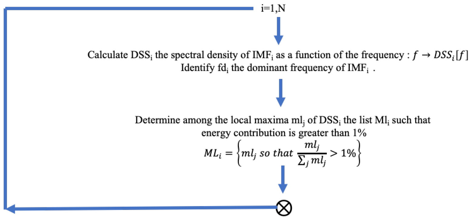
Figure 1Estimation of the spectral density for each IMF spectrum and selection of significant local maxima whose energy contribution >1 %.
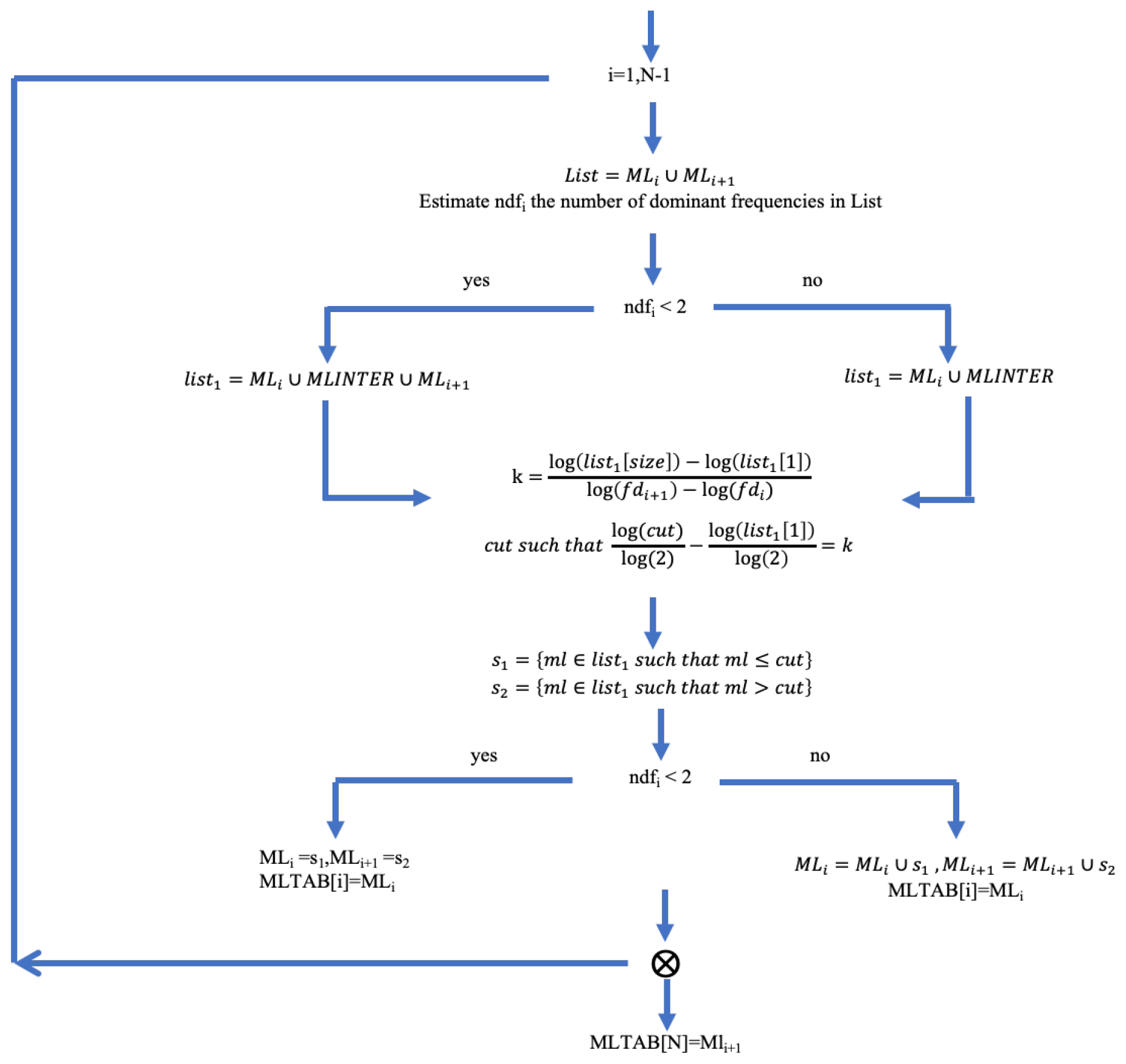
Figure 2Calculation of the MLTAB matrix. Each row of MLTAB contains the list of significant local maxima present in the spectrum of an IMF. The rows of MLTAB have no common elements, and therefore MLTAB can be seen as a set of non-overlapping local maximum groups and represents a segmentation of the original signal Fourier spectrum.
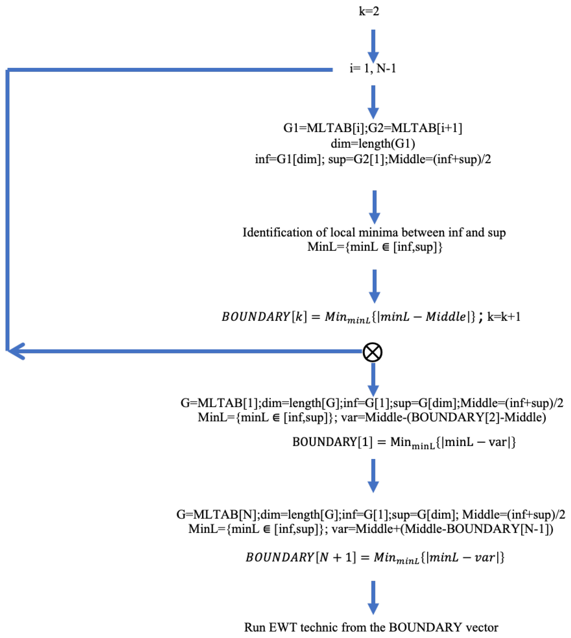
Figure 3Calculation of the BOUNDARY vector representing the boundaries between the local maximum groups contained in the MLTAB matrix. The EWT technique is run from BOUNDARY.
“Size” represents the length of list1 and “cut” is the boundary between two consecutive local maximum groups MLi and MLi+1.
The parameter k can be interpreted as the ratio between the number of scales contained in list1 and the number of scales in the interval [fdi, fdi+1] of two consecutive dominant frequencies.
The EMD and EAWD techniques presented above have been applied to two experimental time series of observations. The first time series was a series of monthly total columns of ozone (TCO) in Dobson units (DU), recorded over 41 years, from January 1979 to December 2019, by a SAOZ (Zenithal Observation Analysis System) spectrometer on the Moufia University Campus, Saint-Denis, Réunion (21∘ S, 55.5∘ E).
This TCO time series was elaborated by merging satellite data (OMI and TOMS) and ground-based observations recorded by a SAOZ spectrometer (Pommereau and Goutail, 1988) installed in Saint-Denis, Réunion, in 1993. The method used for merging satellite and ground data to obtain a homogeneous series is explained in Pastel et al. (2014).
Despite its low abundance, ozone plays an important role in the Earth's atmosphere. It is mainly produced in the tropical stratosphere and transported to higher latitudes by the large-scale circulation called the Brewer–Dobson circulation. In the stratosphere, ozone acts like a filter and prevents incident solar ultraviolet (UV) radiation from reaching the ground, thus protecting the biosphere. The significant depletion of the ozone layer since the late 1970s has revealed the importance of ozone in the climate system and the associated environmental and health risks. The TCO is a parameter that measures the abundance of ozone over a given location. It is given in DU and consists of ∼90 % stratospheric ozone and ∼10 % tropospheric ozone.
The second time series comprised 57 years of monthly rainfall measurements recorded at the Conakry (Guinea) meteorological station from 1961 to 2017.
The resulting original time series of total ozone columns and rainfall measurements are displayed in Figs. 4 and 5 respectively.

Figure 4Monthly time series of total ozone columns in Dobson units (DU) over Réunion from 1979 to 2019. The time axis is expressed in years.

Figure 5Monthly rainfall record time series recorded in Conakry (Guinea) from 1960 to 2019. The time axis is expressed in years.
Very often, noise is present in the original time series. To deal with this problem, the authors suggest computing an EEMD (Wu and Wang, 2009). This approach seems to reduce the noise present in the original signal. Generally, some of the IMFs returned by the EEMD technique present poor correlations with the original signal and therefore make a weak contribution to the variability of the original series. Such IMFs are qualified as irrelevant. Relevant IMFs are discriminated from the irrelevant ones by means of two criteria. The first of these criteria uses Pearson's correlation to estimate the degree of correlation of each IMF with the original signal by setting a threshold. A threshold commonly used in the literature (Ayenu-Prah and Attoh-Okine, 2010) can be expressed as:
In Eq. (13), Cor(IMFi,x) stands for the Pearson correlation coefficient between the ith IMF and the original signal x(t), i.e.
where SD represents the standard deviation and Cov the covariance.
The second criterion determines the energy contribution of each IMF compared with the energy contained in the original signal. The energy contribution of each IMF is calculated as a percentage as follows:
where because each IMF is a zero-mean function by construction. .
The threshold set for this second criterion is 1 %.
IMFs with a degree of correlation less than τ and for which the energy contribution is less than 1 % are said to be irrelevant. The irrelevant IMFs are added to the residual mode R returned by the EEMD to form the trend of the original signal. For such IMFs to be part of the trend of the observed dynamics, they must not be too oscillating and are therefore contiguous to the residue.
When EEMD was applied to the Réunion TCO time series presented in Fig. 4, seven IMFs were found in addition to the residual mode. Taking account of the selection procedure mentioned above, the first five of the seven IMFs initially identified were relevant, and IMFs 6 and 7 were added to the residual mode. Results are displayed in Fig. 6 below.
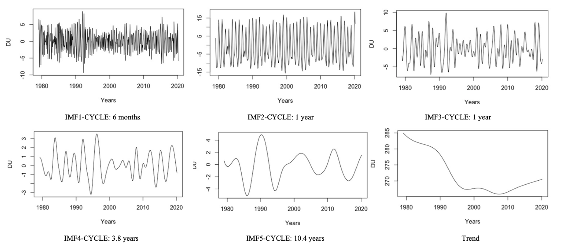
Figure 6Relevant IMFs and trend from the EEMD applied to time series of Réunion total columns of ozone from 1979 to 2019.
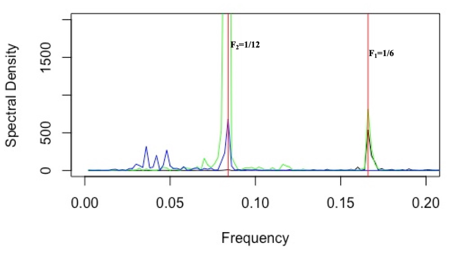
For each IMF, the cycle defined as the period associated with the dominant frequency is specified. Mode mixing occurs in IMF2 and IMF3 as they have the same 1-year oscillation cycle. As shown in Fig. 7, the IMF2 spectrum contains and frequencies, and F2 is contained in both IMF2 and IMF3.
To estimate the accuracy of the residual returned by the EEMD, it is compared with the trend of the original signal obtained from a moving window with a size set at the maximum of the relevant IMF cycles, i.e. 125 months (10.4 years).
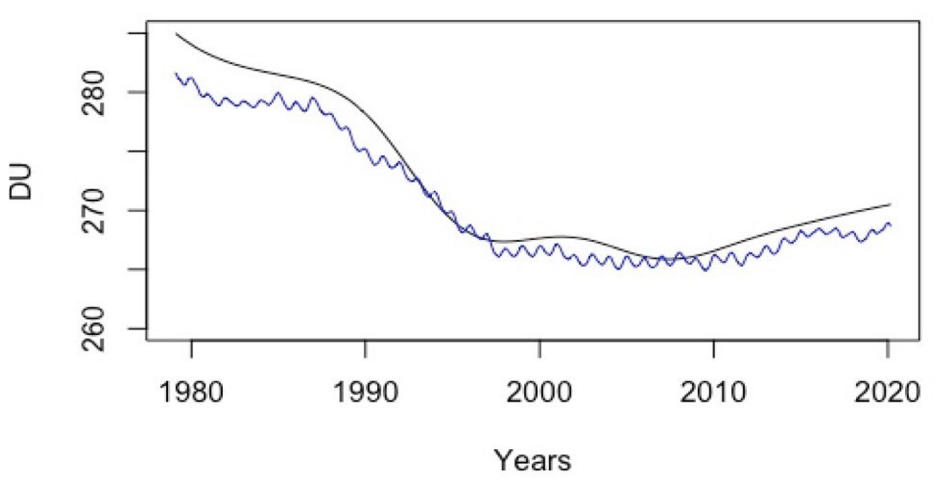
Figure 8Trend obtained from the EEMD technique (black curve). The trend of the original signal obtained from a moving window (blue curve) with a 125-month size (i.e. 10.4 years).
The accuracy of the residual, R, returned by the EEMD and compared with the trend of the original signal by using a moving window, Tmb, was estimated using the following expression:
where N is the original time series length and represents the mean operator.
To overcome the mixing mode occurring in IMFs 2 and 3 returned by the EEMD technique, we applied the EAWD technique to the Réunion TCO time series. The results obtained with EAWD are displayed in Fig. 9 below.
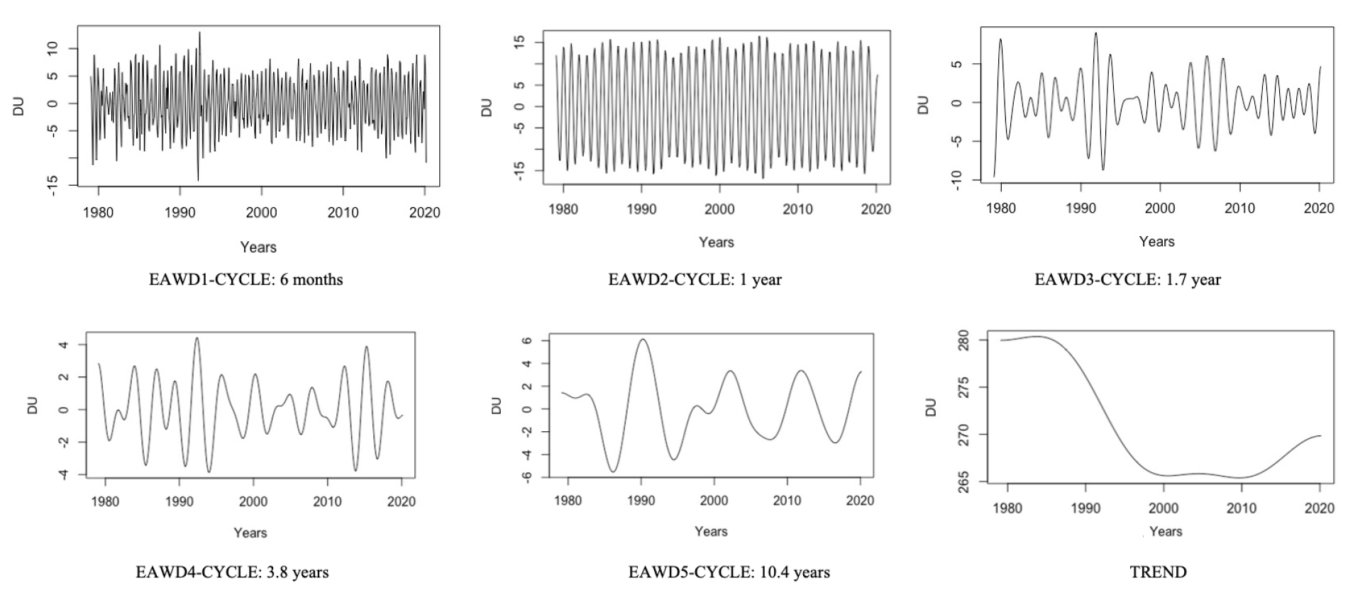
As shown in Fig. 10 below, the 6-month and 1-year cycles relating respectively to EAWD1 and EAWD2 are correctly separated, and the mode mixing occurring in the EEMD results has been removed.
Similarly, the accuracy of the residual returned by the EAWD technique was estimated and compared with that returned by the EEMD.
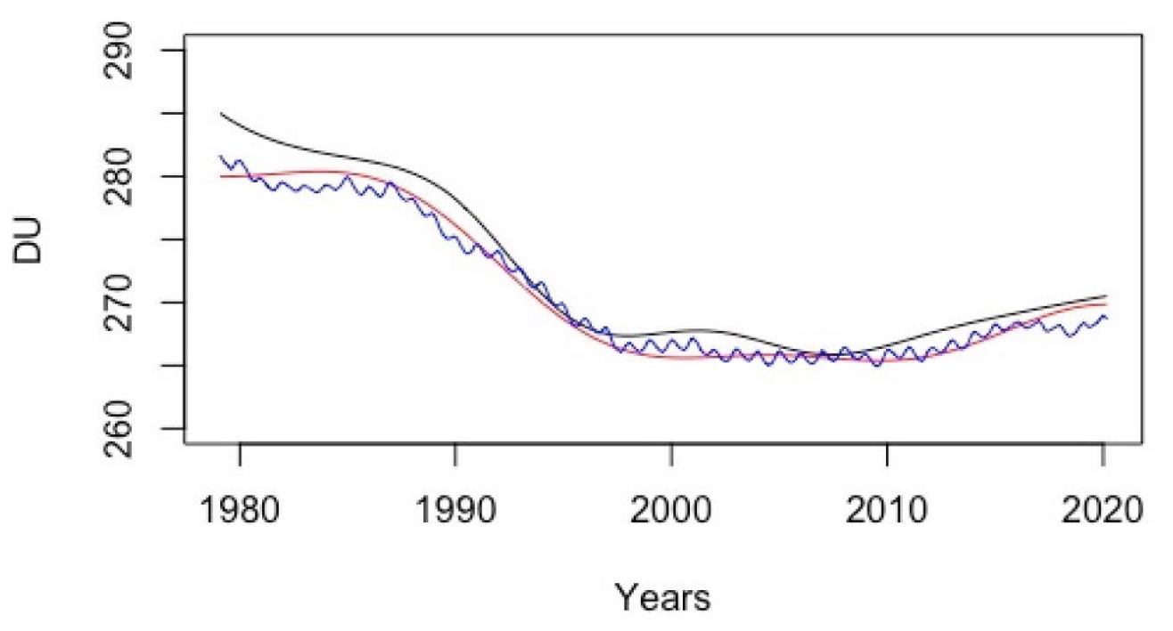
Figure 11The residual TrendEAWD returned by the EAWD technique (red curve), the trend of the original signal obtained from a moving window (blue curve) with a size fixed at 125 (i.e. 10.4 years), and the residual returned by the EEMD technique (black curve).
Likewise, the accuracy of the residual returned by the EAWD technique was estimated using Eq. (16): PrEAWD=0.3 %.
The EAWD trend expressed in DU per decade is shown in Fig. 12.
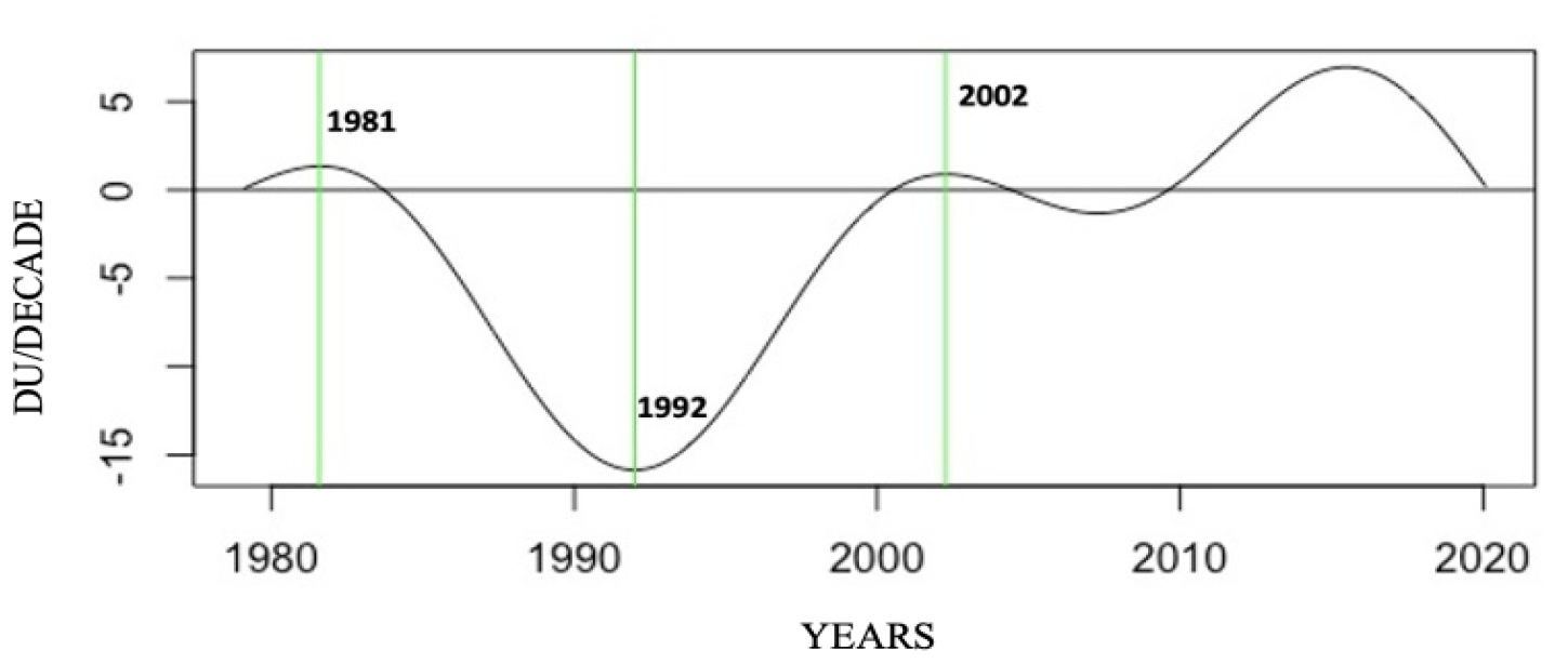
Results in Fig. 12 show that ozone levels in Réunion decreased from 1981, stopped decreasing in 1992, and started rising again from 2002.
The accuracy of the DU per decade EAWD trend in Fig. 12 was calculated as 2×PrEAWD, i.e. 0.6 %.
EEMD was applied to the rainfall time series measurements, and relevant IMFs were selected. Results are represented in Fig. 13 below.
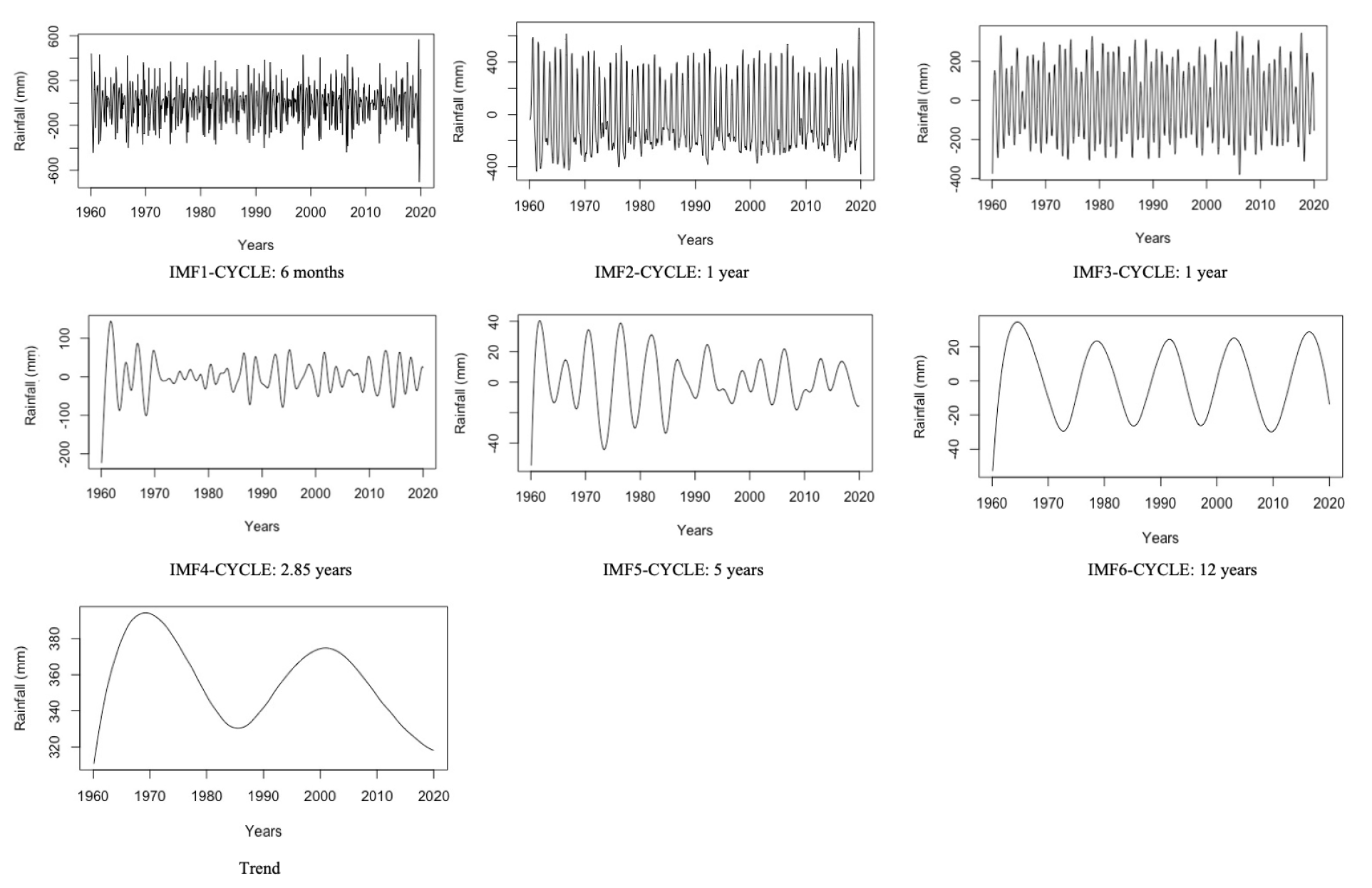
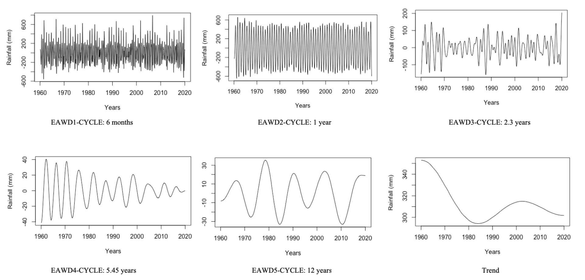
Figure 13Relevant IMFs and trend from the EEMD applied to the Conakry rainfall time series from 1960 to 2019.
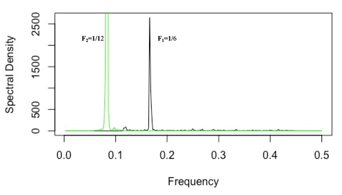
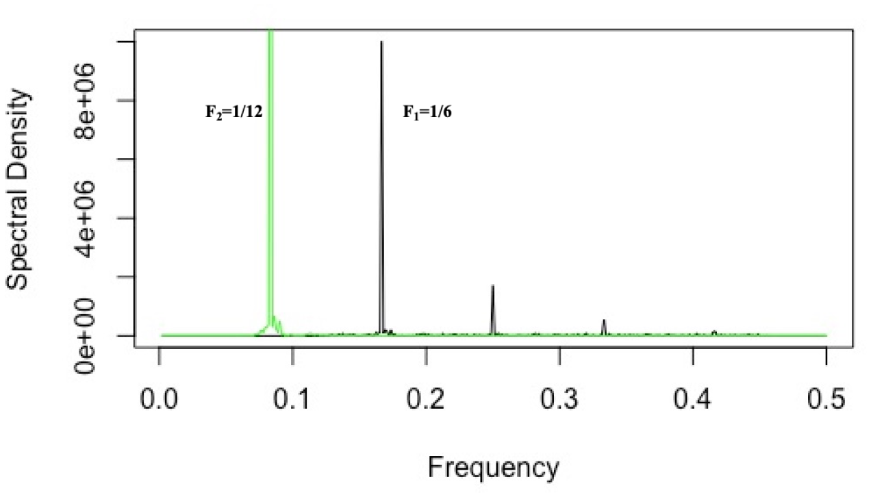
Mode mixing occurs in IMF2 and IMF3 as they have the same 1-year oscillation cycle. As shown in Fig. 14 below, frequency is contained in both IMF1 and IMF2, while is contained in IMF1, IMF2, and IMF3.
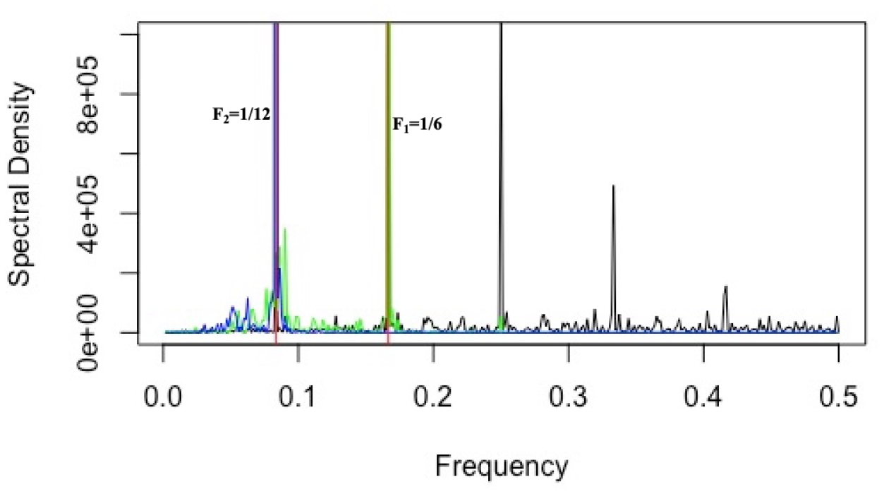
Figure 14Rainfall IMF1 (black line), IMF2 (green line), and IMF3 (blue line) spectral contents.
The accuracy of the trend calculated from EEMD results is compared below with the trend of the original signal obtained from a moving window with its size set at the maximum of the relevant IMF cycles, i.e. 144 months (12 years).
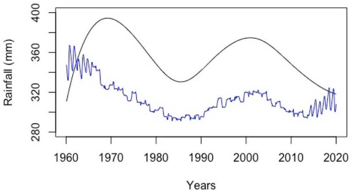
Figure 15Trend obtained from the EEMD technique (black curve) with the trend of the original signal obtained from a moving window (blue curve) with a size of 144 months (i.e. 12 years).
The accuracy of the residual returned by the EEMD technique was estimated using Eq. (16): PrEEMD=15 %.
Results obtained with EAWD are displayed in Fig. 16 below.
The 6-month and 1-year cycles relating respectively to EAWD1 and EAWD2 are correctly separated, and the mode mixing occurring in the EEMD results has been removed (see Fig. 17).
The accuracy of the residual returned by the EAWD technique was estimated at PrEAWD=0.9 %.
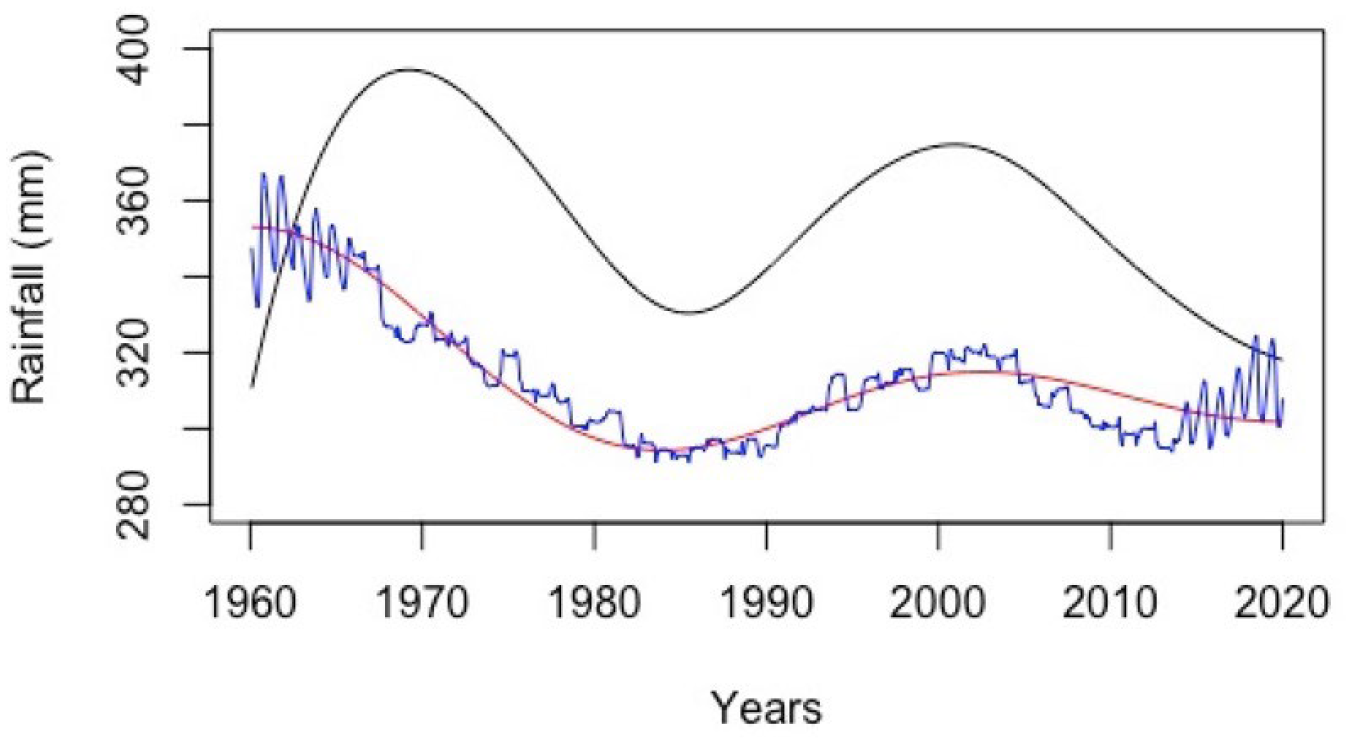
Figure 18The residual TrendEAWD returned by the EAWD technique (red curve), the trend of the original signal obtained from a moving window (blue curve) with a size fixed at 144 (i.e. 12 years), and the residual returned by the EEMD technique (black curve).
The EAWD trend represented by an annual average of rainfall (in millimetres) is shown in Fig. 19 below.
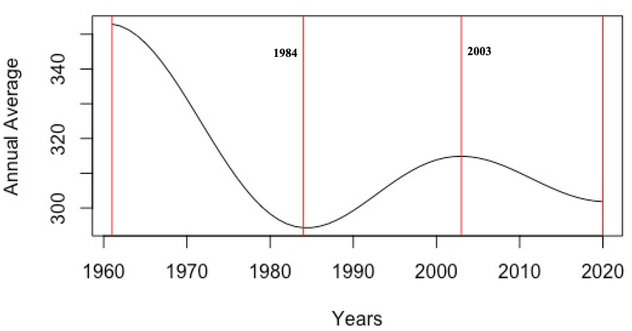
The results reported in Fig. 19 show that the rainfall average amount decreased by 2.3 mm yr−1 in the period [1960, 1984], then increased by 1 mm yr−1 in the period [1984, 2003], and decreased again, by 0.7 mm yr−1, in the period [2003, 2020].
The method commonly employed in atmospheric physics to determine the variability and trend of observation time series is to use a multi-linear regression model. This type of approach has been used very often (Randel and Thompson, 2011; Bourassa et al., 2014; Toihir et al., 2018).
The main requirement of this method is the a priori knowledge of the atmospheric climate forcings that control the variability of the time series studied. The ozone–QBO (Quasi-Biennial Oscillation) relationship has been discussed in several papers, as has the influence of ENSO (El Niño–Southern Oscillation) on ozone variability (Butchart et al., 2003; Brunner et al., 2006; Randel and Thompson, 2011). Other papers have shown the role played by solar flux in the temporal variability of ozone (Randel and Wu, 2007).
To validate results obtained with the EAWD method on the TCO time series for Réunion, we used the TREND-RUN multi-linear regression model developed at the University of Réunion and already applied in many studies (Bencherif et al., 2006; Bègue et al., 2010; Toihir et al., 2018).
Climate forcings used as input to the TREND-RUN model were QBO, ENSO, and solar flux. A linear function was used to estimate the long-term linear trend of the series. The trend was then estimated by calculating the slope of the normalized linear function. As the variability of ozone is also affected by the annual and semi-annual oscillations (AO and SAO), these two analytic oscillations were also used as input to the model. The TREND-RUN model and the climate forcings used (such as ENSO, QBO, and solar flux at 10.7 cm) are described in detail in Toihir et al. (2018).
The results obtained here with TREND-RUN on the 1979–2019 Réunion TCO time series are consistent with those obtained by Toihir et al. (2018) on a shorter total ozone series at Réunion (1998–2013).
The trend obtained from the TREND-RUN model over the whole monthly mean ozone series from 1979 to 2019 is % per decade. The error is estimated from the SD of the residual found by the model.
The variability components returned by the EAWD method are in agreement with the climatic forcings used as input to the TREND-RUN model, and the energy contributions respectively estimated by the TREND-RUN model and the EAWD technique are reported in Table 1.
Table 1Comparison of total ozone variability in Réunion (from 1979 to 2019) obtained with the TREND-RUN model and the EAWD method.
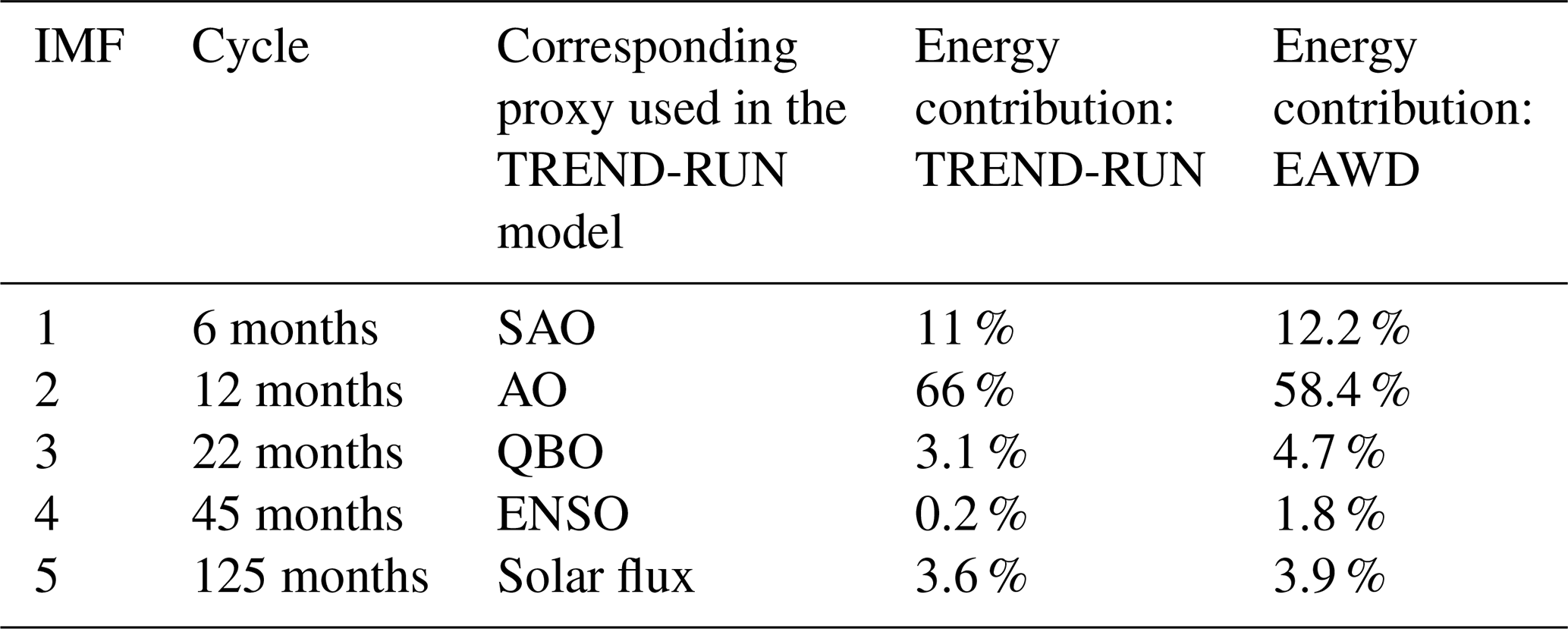
The main advantage of the EAWD technique for analysing the ozone variability from an observational time series is that it auto-adaptively extracts the modes of variability implicitly contained in the original time series without requiring any a priori knowledge of the atmospheric forcings controlling the ozone variability. It can be seen that the results returned by the EAWD method are in complete agreement with those returned by the TREND-RUN model. On the other hand, the energy contributions of the various modes of variability obtained with the EAWD method are compatible with those obtained with the TREND-RUN method (Table 1).
In contrast to the trend returned by the TREND-RUN model, which is linear over the whole duration of the series, the EAWD technique enables the evolution of the trend to be visualized over the whole period studied.
TREND-RUN has not been applied to the Conakry rainfall time series as it contains intermittent processes, which makes use of multi-linear methods inappropriate.
EMD is a method for breaking down a signal without leaving the time domain. It can be compared with other analysis methods, such as Fourier transforms and wavelet decomposition, and the process is very useful for analysing raw signals, which are most often non-linear and non-stationary. Even though the EMD adaptability seems useful for many applications, the major drawback with EMD lies in the mode mixing, where the spectral contents of IMFs overlap each other. To overcome this problem, the EWT technique proposes a new approach, introducing a way of building adaptive wavelets and thus of extracting the different oscillatory modes from a signal by designing an appropriate filter bank. At the heart of the EWT technique lies the segmentation of the Fourier spectrum of the original signal. The main idea of the proposed EAWD technique is to use the results provided by EMD to segment the Fourier spectrum of the original signal. The algorithm implemented uses the spectral contents of the IMFs and ensures that their supports do not overlap, so that they can constitute a segmentation of the Fourier spectrum of the original signal. In another way, the method most commonly used to analyse the variability of observation time series is based on a multi-linear regression model. If we look at the results obtained with the TREND-RUN model on Réunion TCO time series, the variability modes returned by the EAWD are in good agreement with those obtained with the TREND-RUN multi-linear regression model.
From a comparison between the results obtained with the EMD and EAWD techniques, it emerges that the EAWD technique enables the mode-mixing problem to be overcome while providing a trend with better accuracy than that obtained with the EMD technique. Thanks to the rigour of the EWT, the EAWD keeps the behaviour of the signal in the timescales returned by the EMD. In this context, the EAWD technique can be seen as an optimization of the EMD.
The first version of the EAWD method was written in R and is currently a beta version of the code and still requires some validation so that it can run on any time series before being included in an R package.
The data are available from Thierry Portafaix and Hassan Bencherif at LACy UMR 8105 University of Reunion.
OD and AB developed and implemented the EAWD method. EL conducted the test and numerical validation. TP and HB conducted physical validation and comparison between the EAWD results with those obtained with a multilinear regression model.
The contact author has declared that neither they nor their co-authors have any competing interests.
Publisher’s note: Copernicus Publications remains neutral with regard to jurisdictional claims in published maps and institutional affiliations.
This study has been funded by the LEFE French National programme.
This paper was edited by Norbert Marwan and reviewed by two anonymous referees.
Ayenu-Prah, A. Y. and Attoh-Okine, N.: A Criterion for Selecting Relevant Intrinsic Mode Functions in Empirical Mode Decomposition, Advances in Adaptive Data Analysis, 2, 1–24, https://doi.org/10.1142/S1793536910000367, 2010.
Bègue, N., Bencherif, H., Sivakumar, V., Kirgis, G., Mze, N., and Leclair de Bellevue, J.: Temperature variability and trends in the UT-LS over a subtropical site: Reunion (20.8∘ S, 55.5∘ E), Atmos. Chem. Phys., 10, 8563–8574, https://doi.org/10.5194/acp-10-8563-2010, 2010.
Bencherif, H., Diab, R. D., Portafaix, T., Morel, B., Keckhut, P., and Moorgawa, A.: Temperature climatology and trend estimates in the UTLS region as observed over a southern subtropical site, Durban, South Africa, Atmos. Chem. Phys., 6, 5121–5128, https://doi.org/10.5194/acp-6-5121-2006, 2006.
Bourassa, A. E., Degenstein, D. A., Randel, W. J., Zawodny, J. M., Kyrölä, E., McLinden, C. A., Sioris, C. E., and Roth, C. Z.: Trends in stratospheric ozone derived from merged SAGE II and Odin-OSIRIS satellite observations, Atmos. Chem. Phys., 14, 6983–6994, https://doi.org/10.5194/acp-14-6983-2014, 2014.
Brunner, D., Staehelin, J., Maeder, J. A., Wohltmann, I., and Bodeker, G. E.: Variability and trends in total and vertically resolved stratospheric ozone based on the CATO ozone data set, Atmos. Chem. Phys., 6, 4985–5008, https://doi.org/10.5194/acp-6-4985-2006, 2006.
Butchart, N., Scaife, A. A., Austin, J., Hare, S. H. E., and Knight, J. R.: Quasi-biennial oscillation in ozone in a coupled chemistry-climate model, J. Geophys. Res., 108, 4486, https://doi.org/10.1029/2002JD003004, 2003,
Daubechies, I.: Ten Lectures on Wavelets, in: CBMS-NSF Regional Conference Series in Applied Mathematics, Society for Industrial and Applied Mathematics, ISBN: 978-0-89871-274-2, 1992.
Delage, O., Portafaix, T., Bencheriff, H., Guimbretière, G., and Loua, R. T.: Multi-scale Variability Analysis of Time Series in Geophysics by using the Empirical Mode Decomposition, Processing SAGA, https://hal.archives-ouvertes.fr/hal-02363170, last access: 6 October 2019.
Flandrin, P., Rilling, G., and Gonçalvès, P.: Empirical Mode Decomposition as a filter bank, IEEE Signal Proc. Let., 11, 112–114, 2004.
Fosso, O. B. and Molinas, M.: Method for mode mixing separation in Empirical Mode decomposition, arXiv [preprint], arXiv:1709.05547v1, 16 September 2017.
Gao, Y., Ge, G., Sheng, Z., and Sang, E.: Analysis and solution to the mode mixing phenomenon in EMD, in: 2008 Congress on Image and Signal Processing, Sanya, China, 27–30 May 2008, https://doi.org/10.1109/CISP.2008.193, 2008.
Gilles, J.: Empirical Wavelet Transform, IEEE T. Signal Proces., 61, 3999–4010, https://doi.org/10.1109/TSP.2013.2265222, February 2013.
Huang, N. E., Shen, Z., Long, S. R., Wu, M. C., Shih, H. H., Zheng, Q., Yen, N.-C., Tung, C. C., and Liu, H. H.: The empirical mode decomposition and the Hilbert spectrum for nonlinear and non-stationary time series analysis, P. Roy. Soc. Lond. A, 454, 903–995, 1998.
Jaffard, S., Meyer, Y., and Ryan, R. D.: Wavelets: Tools for Science and Technology, SIAM, ISBN: 0898714486, 2001.
Meyer, Y.: Wavelets, Vibrations and Scaling, American Mathematical Society, Centre de Recherches Mathématiques, ISBN: 978-0821806852, 1997.
Pastel, M., Pommereau, J.-P., Goutail, F., Richter, A., Pazmiño, A., Ionov, D., and Portafaix, T.: Construction of merged satellite total O3 and NO2 time series in the tropics for trend studies and evaluation by comparison to NDACC SAOZ measurements, Atmos. Meas. Tech., 7, 3337–3354, https://doi.org/10.5194/amt-7-3337-2014, 2014.
Pommereau, J.-P. and Goutail, F.: Ground-based measurements by visible spectrometry during Arctic Winter and Spring, Geophys. Res. Lett., 15, 891–894, https://doi.org/10.1029/GL015i008p00891, 1988.
Randel, W. J. and Thompson, A. M.: Interannual variability and trends in tropical ozone derived from SAGE II satellite data and SHADOZ ozonesondes, J. Geophys. Res., 116, D07303, https://doi.org/10.1029/2010JD015195, 2011.
Randel, W. J. and Wu, F.: A stratospheric ozone profile data set for 1979–2005: Variability, Trends and comparison with column ozone data, J. Geophys. Res., 112, D06313, https://doi.org/10.1029/2006jd007339, 2007.
Toihir, A. M., Portafaix, T., Sivakumar, V., Bencherif, H., Pazmiño, A., and Bègue, N.: Variability and trend in ozone over the southern tropics and subtropics, Ann. Geophys., 36, 381–404, https://doi.org/10.5194/angeo-36-381-2018, 2018.
Wu, Z. and Huang, N. E.: Ensemble empirical mode decomposition: A noise-assisted data analysis method, Advances in Adaptive Data Analysis, 1, 1–41, https://doi.org/10.1142/S1793536909000047, 2009.
- Abstract
- Introduction
- The existing approaches
- The empirical adaptive wavelet decomposition (EAWD)
- Time series analysis and results
- Consistency of the EAWD method
- Conclusion
- Code availability
- Data availability
- Author contributions
- Competing interests
- Disclaimer
- Financial support
- Review statement
- References