the Creative Commons Attribution 4.0 License.
the Creative Commons Attribution 4.0 License.
 | 14 Oct 2021
Identification of linear response functions from arbitrary perturbation experiments in the presence of noise – Part 1: Method development and toy model demonstration
Guilherme L. Torres Mendonça
Julia Pongratz
Christian H. Reick
Existent methods to identify linear response functions from data require tailored perturbation experiments, e.g., impulse or step experiments, and if the system is noisy, these experiments need to be repeated several times to obtain good statistics. In contrast, for the method developed here, data from only a single perturbation experiment at arbitrary perturbation are sufficient if in addition data from an unperturbed (control) experiment are available. To identify the linear response function for this ill-posed problem, we invoke regularization theory. The main novelty of our method lies in the determination of the level of background noise needed for a proper estimation of the regularization parameter: this is achieved by comparing the frequency spectrum of the perturbation experiment with that of the additional control experiment. The resulting noise-level estimate can be further improved for linear response functions known to be monotonic. The robustness of our method and its advantages are investigated by means of a toy model. We discuss in detail the dependence of the identified response function on the quality of the data (signal-to-noise ratio) and on possible nonlinear contributions to the response. The method development presented here prepares in particular for the identification of carbon cycle response functions in Part 2 of this study (Torres Mendonça et al., 2021a). However, the core of our method, namely our new approach to obtaining the noise level for a proper estimation of the regularization parameter, may find applications in also solving other types of linear ill-posed problems.
- Article
(5349 KB) - Full-text XML
- Companion paper
- BibTeX
- EndNote


To gain understanding of a physical system, it is very helpful to know how it responds to perturbations. Considering a small time-dependent perturbation , the resulting time-dependent response can from a very general point of view be written as
where the linear response function is a characteristic of the considered system. In fact, under a number of assumptions – among which smoothness and causality are the most important – Eq. (1) is the first term of a functional expansion of the response R into the perturbation f around the unperturbed state , known as Volterra series (Volterra, 1959; Schetzen, 2010). In this framing, the key to gaining insight into the system is the linear response function χ: by knowing this function one has at hand not only a powerful tool to predict the response for sufficiently small but otherwise arbitrary perturbations, but also a means to study the internal dynamic modes of the unperturbed system by analyzing the temporal structure of the response function.
Linear response functions have been successfully applied within different contexts in many fields of science and technology. In physics, for example, material constants like the magnetic susceptibility or the dielectric function must be understood as linear response functions that can be obtained by Kubo's theory of linear response (Kubo, 1957) via the fluctuation–dissipation theorem from an auto-correlation of the unperturbed system. However, applications of these functions range far beyond physics into fields like neurophysiology and climate (Gottwald, 2020). In climate science, in particular, applications of linear response functions in the context of Ruelle's developments in response theory (see below) are a recent topic (e.g., Lucarini, 2009; Lucarini and Sarno, 2011; Lucarini et al., 2014; Ragone et al., 2016; Lucarini et al., 2017; Aengenheyster et al., 2018; Ghil and Lucarini, 2020; Lembo et al., 2020; Bódai et al., 2020). On the other hand, these functions have already been successfully employed as a heuristic tool to study climate and the carbon cycle for decades (e.g., Siegenthaler and Oeschger, 1978; Emanuel et al., 1981; Maier-Reimer and Hasselmann, 1987; Enting, 1990; Joos et al., 1996; Joos and Bruno, 1996; Thompson and Randerson, 1999; Pongratz et al., 2011; Caldeira and Myhrvold, 2013; Joos et al., 2013; Ricke and Caldeira, 2014; Gasser et al., 2017; Enting and Clisby, 2019). Yet another perspective is that from engineering sciences, in which the impulse response – that to a large extent corresponds to the linear response function – and the closely related transfer function (or system function) characterize linear time-invariant (LTI) systems, widely applied in fields such as signal processing and control theory (Kuo, 1966; Rugh, 1981; Beerends et al., 2003; Boulet and Chartrand, 2006). Regardless of which viewpoint a particular community takes to investigate the linear response of a system, a fundamental step in this investigation is the identification of the appropriate linear response function, the topic of the present study.
From a theoretical point of view, the existence of a linear response is by no means obvious: structurally stable dynamical systems are the exception (Abraham and Marsden, 1982), so that already small parameter changes typically lead to topological changes in their sets of stable and unstable solutions. Not every such bifurcation must prevent a linear response in macroscopic observables, but the question remains how in view of microscopic structural instability macroscopic linearity can prevail. A key result in this field is Ruelle's rigorous demonstration of the existence of a linear response for the structurally stable class of uniform hyperbolic systems (Ruelle, 1997, 1998). It is believed that this result transfers to large classes of nonequilibrium systems (Ruelle, 1999; Lucarini, 2008; Lucarini and Sarno, 2011; Gallavotti, 2014; Ragone et al., 2016; Lucarini et al., 2017). An example may be the Lorenz system at standard parameters, for which numerical analysis revealed evidence for a linear response despite non-hyperbolicity (Reick, 2002; Lucarini, 2009). Recent investigations by Wormell and Gottwald (2018, 2019) indicate that the thermodynamic limit must be invoked to reconcile microscopic structural instability with macroscopic differentiability. Results on the existence/absence of a linear response have been particularly obtained for iterative maps (Großmann, 1984; Baladi, 2018; Śliwiak et al., 2021), which are known for their notoriously rich bifurcation structure. Well studied is also the linear response of stochastic systems (Hänggi and Thomas, 1982; Risken, 1996) for whose quasistatic response rigorous mathematical results also exist (Hairer and Majda, 2010).
In practical applications where the response function must be recovered from data, its identification may be a challenging task. The reason is that the identification problem is generally ill-posed, so that by classical numerical methods one obtains a recovery severely deteriorated by noise (see below). In addition, existent methods to identify these functions from data require one to perform special perturbation experiments. In the present study, we develop a method to identify linear response functions, taking data from any type of perturbation experiment while fully accounting for the ill-posedness of the problem.
The generality of our method allows for derivation of response functions in cases hardly possible before. Examples are problems where performing perturbation experiments is computationally expensive, so that one must use data that were not designed for the purpose of deriving these functions. In the geosciences, this may be the case when one is interested in characterizing by response functions the dynamics of Earth system models – extremely complex systems employed to simulate climate and its coupling to the carbon cycle. In principle, with our method one can derive these functions, taking simulation data from Earth system model intercomparison exercises such as C4MIP – the Coupled Climate-Carbon Cycle Model Intercomparison Project (Taylor et al., 2012; Eyring et al., 2016) – that are already available in international databases. In Part 2 of this study we explore this possibility by investigating in an Earth system model the response of the land carbon cycle to atmospheric CO2 perturbations. Because of the relationship between the linear response function and the impulse response and the transfer function in LTI systems, our work can also be seen from the viewpoint of the engineering sciences as a contribution to the corpus of methods to solve system identification problems (Åström and Eykhoff, 1971; Söderström and Stoica, 1989; Isermann and Münchhof, 2010; Pillonetto et al., 2014).
In the field of climate science, the typical method to identify linear response functions is by means of the impulse response function, which is the response to a Dirac delta-type perturbation (e.g., Siegenthaler and Oeschger, 1978; Maier-Reimer and Hasselmann, 1987; Joos et al., 1996; Thompson and Randerson, 1999; Joos et al., 2013). This method has become so widely known that often the terms linear response function and impulse response function are used interchangeably. Indeed, in the particular case where perturbations are weak, the two concepts coincide. However, this is not true in general: if the impulse strength is large so that nonlinearities become important, the impulse response function differs from the linear response function.
Other studies have proposed to identify linear response functions by making use of other types of perturbations. Reick (2002) and Lucarini (2009) used a weak periodic forcing to derive response functions in the Fourier space (also called susceptibilities). Hasselmann et al. (1993), Ragone et al. (2016), MacMartin and Kravitz (2016), Lucarini et al. (2017), Van Zalinge et al. (2017), Aengenheyster et al. (2018), and Bódai et al. (2020) identify the linear response function using step experiments, where the perturbation is a Heaviside-type function. Additional studies have proposed to compute the linear response of the system using the invariant measure of the unperturbed system (Gottwald et al., 2016) and by means of shadowing methods (Reick, 1996; Ni and Wang, 2017; Ni, 2020).
As noted by Lucarini et al. (2014), in principle the linear response function of a system can be derived by taking data from an arbitrary type of perturbation experiment. One method would be to apply a Laplace transform to Eq. (1), so that χ(t) can in principle be computed by the inverse Laplace transform
where ℒ{⋅} is the Laplace transform operator. In fact, a first step towards the derivation of χ(t) from the general Eq. (1) was taken by Pongratz et al. (2011), although the problem was not systematically discussed.
Deriving χ(t) from perturbation experiment data is not a trivial problem. For the general case where the perturbation is different from a Dirac delta-type function, the problem is ill-posed (e.g., Bertero, 1989; Landl et al., 1991; Lamm, 1996; Engl et al., 1996). This basically means that attempts to recover the exact χ(t) yield a solution with large errors due to an amplification of the noise in the data. On the other hand, when f(t) is a Dirac delta-type function with sufficiently small perturbation strength, so that the response can be considered linear, the impulse response gives directly the linear response function, i.e., χ(t)=R(t). However, even in this case noise may hinder the recovery: because the perturbation is only one “pulse” with small perturbation strength, the response may have a too low signal-to-noise ratio because of internal variability (Joos et al., 2013), giving once more a recovery with large errors.
To remedy these noise problems, a method intended to “damp” the noise in the response is usually employed. In MacMartin and Kravitz (2016), a step experiment with large perturbation strength is used to obtain a better signal-to-noise ratio in the response but at the cost of enhancing the effect of nonlinearities. An alternative approach is employed by Ragone et al. (2016) and Lucarini et al. (2017), who employ an ensemble of simulation experiments and take the ensemble-averaged response so that the level of noise is reduced. However, especially for complex models such as Earth system models, ensembles of simulations can be computationally extremely expensive, so that such a procedure may not be feasible.
Instead of trying to improve the signal-to-noise ratio of the data by improved experiment design, here we are interested in deriving χ(t) from a single realization of a given experiment by accounting for the ill-posedness of the problem. For this purpose, we employ regularization theory. Although this theory offers a variety of methods to solve ill-posed problems (see, e.g., Groetsch, 1984; Bertero, 1989; Bertero et al., 1995; Engl et al., 1996; Hansen, 2010), currently no general all-purpose method exists. Typically, methods rely on some type of prior information about the problem (Istratov and Vyvenko, 1999). Hence, they must be tailored according to the particularities of each application. Here, we develop a method that under certain assumptions solves the ill-posed problem when, in addition to the data from a single arbitrary perturbation experiment, data from an associated unperturbed – or control – experiment are also given to obtain independent information about the noise level (Sect. 3). First, we assume that the response function is well approximated by a sum of decaying exponentials, meaning that potential oscillatory contributions to the response function are so small that they can be considered to be part of the noise. The response function is obtained by applying Tikhonov–Phillips regularization. The regularization parameter is chosen via the discrepancy method. An essential ingredient of the discrepancy method is the noise level, which is usually not known a priori. For this reason, we propose a method to estimate the noise level by taking advantage of the information given by a spectral analysis of the perturbation experiment and the control experiment. If the desired response function is known to be monotonic, the noise estimate can be further adjusted. In Sect. 4, the method is demonstrated to give reliable results under appropriate conditions of noise and nonlinearity. In Sect. 5, we compare the derived method with two existent methods in the literature to identify the response function in the time domain. Results and technical details are discussed in Sect. 6. Additional calculations are shifted to the Appendices.
As a preparation for introducing our method in Sect. 3, in the present section we derive its basic ansatz, which takes into account, in addition to the response formula (Eq. 1), also the noise in the data. Depending on the application context, the noise may arise for different reasons, such as errors in the measurements or stochastic components in the system. As will be seen, our basic ansatz is in principle applicable to all those cases. However, to make the connection to modern applications of linear response functions that arise in the context of Ruelle's developments (e.g., climate), here we derive this ansatz starting from considerations of linear response theory (Ruelle, 2009). Ruelle considered systems of type
where x(t) is the possibly infinite dimensional state vector and the perturbation f(t) couples to the unperturbed system via the field A1(x). In the present context Eq. (3) could, e.g., represent the dynamics of the Earth system perturbed by anthropogenic emissions f(t). Considering an observable Y(x), Ruelle proved that the ensemble average of its deviation from the unperturbed system 〈ΔY〉 can be expanded in the perturbation f(t):
where the order symbol 𝒪(f2) represents terms that vanish in the limit more quickly than the leading linear term. This expansion describes the response of a system that is noisy as a result of its chaotic evolution: starting from different initial states, one obtains different values for ΔY(x(t)). Compared to Eq. (1), in Eq. (4) the linear response function does not describe the response in observables directly, but only in their ensemble average, i.e., in an average over the initial states of the unperturbed system. For the recovery of linear response functions from numerical experiments, this would mean that one had to perform many experiments starting from different initial states to obtain the appropriate ensemble averages. Using tailored perturbation experiments, it was demonstrated in several studies (e.g., Ragone et al., 2016; Lucarini et al., 2017; Bódai et al., 2020) that linear response functions can indeed be obtained in this way but at the expense of a large numerical burden from the need to perform many experiments. Instead, the aim here is to obtain the linear response functions from a given experiment and only from a single realization. Since we are dealing with a single realization, Eq. (4) becomes
where η(t) is a noise term that must show up as a consequence of dropping the ensemble average. Accordingly, the noise η(t) is introduced here as the difference between the noisy response in a single realization ΔY(t) and the response in the ensemble average 〈ΔY(x(t))〉 (compare Eq. 4). In addition, we assume linearity in the perturbation. As a consequence, the present study is based on the ansatz
where now the response ΔY(t) is divided into a deterministic term and a noise term η(t).
The linearity assumption is on purpose: in the present approach to derive the linear response function (see next section), hereafter called the RFI method (response function identification method), we first use Eq. (6) to obtain χ(t) and justify the linearity assumption a posteriori by analyzing how robustly the response can be recovered for different perturbation strengths. Dropping the nonlinear terms has the advantage that one can use the corpus of linear methods to derive χ(t) from Eq. (6). Note that, in practice, however small the perturbation may be, the nonlinear terms do not vanish. Therefore, the contribution of nonlinearities is in this way distributed between χ(t) and η(t), which will be different from the previous χ(t) and η(t) in Eq. (5). How strongly nonlinearities affect the numerical identification of χ(t) depends on the estimation of η(t), which is a crucial part of our RFI method and the main novelty introduced here to deal with the ill-posedness of the problem to identify χ(t).
In addition, although we derived Eq. (6) starting from considerations of linear response theory, it is clear that this ansatz can also be employed in any other context where it may be assumed that the response formula (Eq. 1) applies and that the data are contaminated by additive noise.
In this section we derive the RFI method. As mentioned above, the aim of this method is to obtain the linear response function using data from a single realization of a given perturbation experiment. For this purpose, an essential step is our novel estimation of the noise term η(t), which requires additional data from an unperturbed (control) experiment.
Starting from the ansatz Eq. (6), the method is based on the idea that the noise term η(t) can be estimated using information on the internal variability from the control experiment in combination with a spectral analysis of the perturbation experiment. The identification of the linear response function proceeds as follows: first, we choose a functional form for χ(t). Second, Eq. (6) is discretized for application to the discrete set of time series data, which results in a matrix equation. Then, assuming that the solution obeys the Picard condition (see below), we estimate the high-frequency components of the noise term η(t) in Eq. (6) via a spectral analysis of the matrix equation applied to the data from the perturbation experiment. Next, assuming that the spectral distribution of noise is similar in the control and perturbation experiments, we also estimate the low-frequency components of η(t). The final estimate of η(t) is then used in a regularization procedure to determine the regularization parameter and thereby find an approximate solution for χ(t). In case χ(t) is known to be monotonic, the approximated solution is further adjusted by checking for monotonicity.
This section is organized as follows. In the first subsection, we introduce the assumption for the functional form of the linear response function. In Sect. 3.2, we present the discretized problem. In Sect. 3.3 we briefly review some elements of regularization theory employed in our method, in particular Tikhonov–Phillips regularization (Sect. 3.3.1) and the discrepancy method (Sect. 3.3.2). In Sect. 3.4 we present our noise estimation procedure by which the regularization parameter is determined. Finally, in Sect. 3.5 we show how this procedure can be further improved in the presence of a monotonicity constraint.
3.1 Functional form of the linear response function
In general, the identification of linear response functions from data may be performed either pointwise (e.g., Ragone et al., 2016) or assuming a functional form (e.g., Maier-Reimer and Hasselmann, 1987). Both approaches usually lead to an ill-posed problem and therefore to similar difficulties in finding the solution (see more details in Sect. 3.3.1). Although the RFI method may be applied in either case, here we assume that the response function consists of an overlay of exponential modes. By this ansatz we guarantee from the outset that the response relaxes to zero for t → ∞, which is consistent with the expectation that real systems have finite memory. Besides constraining the function space for the derivation of the response function, another added value of this approach is that in principle it also gives the spectrum of internal timescales of the response.
Assuming this ansatz, the question on the functional form of χ(t) arises. In climate science, it is typically assumed that the response function can be described by only a few exponents (Maier-Reimer and Hasselmann, 1987; Enting and Mansbridge, 1987; Hasselmann et al., 1993, 1997; Grieser and Schönwiese, 2001; Li and Jarvis, 2009; Joos et al., 2013; Colbourn et al., 2015; Lord et al., 2016), i.e.,
where the τi values are interpreted as characteristic timescales and the gi values are their respective weights. τi and gi are then obtained by applying some fitting technique taking a fixed number of terms M. Thus, an important step in this type of approach is to determine a suitable value for M. A common practice is to initially take only a small number of terms M, solve the problem, and then add terms progressively until the addition of a new term does not improve the fit anymore according to some quality-of-fit criterion (e.g., Kumaresan et al., 1984; Maier-Reimer and Hasselmann, 1987; Hasselmann et al., 1993; Pongratz et al., 2011; Colbourn et al., 2015; Lord et al., 2016). Thereby it is assumed that once results stabilize, the information in the data has already been fully exploited, so that fitting of additional terms would be artificial. Nevertheless, finding the parameters τi and gi either from a given χ(t) by Eq. (7) or from ΔY(t) by inserting Eq. (7) into Eq. (1) means solving a special case of a Fredholm equation of the first kind (see Appendix A), which is an ill-posed problem (Groetsch, 1984). This implies that even though the obtained solution may give a very good fit to the data, it may significantly differ from the exact solution (see, e.g., the famous example from Lanczos, 1956, p. 272).
Therefore, to avoid the complication of determining M, we assume instead that the response function is characterized by a continuous spectrum g(τ) (Forney and Rothman, 2012):
Accordingly, we assume that the response is dominated by relaxing exponentials, meaning that potential contributions from oscillatory modes are not distinguishable from noise. By this approach the timescale τ is not an unknown anymore but is given after discretization by a prescribed distribution with M terms covering a wide range of τi values. Thus, only a discrete approximation to the spectrum g(τ) needs to be found. In this way the functional representation is made independently of the question of information content as long as the spectrum of discrete timescales is chosen to be sufficiently large and dense to widely cover the spectrum of internal timescales of the considered system.
This approach has an additional advantage. By prescribing the distribution of timescales, one must not solve a nonlinear ill-posed problem (by solving Eq. 7 for τi and gi) but only a linear ill-posed problem (by solving Eq. 8 only for g(τ)), for which the mathematical theory is fairly well developed (Groetsch, 1984; Engl et al., 1996). Because the problem is linear, the solution is even given analytically (see Sect. 3.3.1), which makes the method very transparent.
3.2 Discretized problem
In view of applications to geophysical systems like the climate or the carbon cycle (Part 2 of this study) that are known to cover a wide range of timescales (Ghil and Lucarini, 2020; Ciais et al., 2013, Box 6.1), it is useful to switch to a logarithmic scale (Forney and Rothman, 2012) by rewriting Eq. (8) in terms of log 10τ:
Hereafter, q(τ) and its discrete version q (see below) will be called the spectrum.
In order to apply the basic Eq. (6) together with Eq. (9) to experiment data, the whole problem needs to be discretized in time and also with respect to the spectrum of timescales. Here we assume the data to be given at equally spaced time steps , , where N is the number of data, while the timescales are assumed to be equally spaced at a logarithmic scale between maximum and minimum values τmax and τmin, i.e.,
where M is the number of timescales. As shown in Appendix B, the resulting discretized equations corresponding to Eqs. (6) and (9) are
and
where ηk stands for the noise. Combining the response data ΔYk, the spectral values qj, and the noise values ηj into vectors ΔY∈ℝN, q∈ℝM, and η∈ℝN, these equations can be written in vector form as
with the components of matrix A given by
Matrix A is known from the prescribed spectrum of timescales τi and the forcings fi. Considering η as a fitting error, in principle one can apply standard linear methods to solve Eq. (13) for the desired spectrum by minimizing
where denotes the Euclidean norm, i.e., . Here we denoted the spectrum as qη instead of q to emphasize that the spectrum found in this way can only be an approximation to the original q depending on the noise present in the data.
Unfortunately, it turns out that solving Eq. (15) is not a trivial task. The first difficulty is that the finite information provided by the data makes the problem underdetermined: ideally one wants to obtain a spectrum q(τ) defined for , but the data ΔY are discrete and cover only a limited time span. However, the most serious issue in identifying χ(t) arises because Eq. (1) is a special case of a Fredholm equation of the first kind (Groetsch, 1984, 2007, see also Appendix A), where the quest for the integral kernel is well known to be an ill-posed problem (see, e.g., Bertero, 1989; Hansen, 1992). This basically means that any solution qη of Eq. (15) obtained via classical numerical methods such as lower-upper (LU) or Cholesky decomposition will be extremely sensitive to even small errors in the data (Hansen, 1992). Therefore, to solve Eq. (15) for the spectrum qη, we invoke regularization.
3.3 Regularization
To treat the ill-posedness of Eq. (15), our RFI method combines techniques from regularization theory with a novel approach to estimate the noise level in the data. To facilitate the understanding of the method, in this section we briefly review these techniques along with some other aspects of the theory that are relevant for our method development.
3.3.1 Regularized solution
To deal with the ill-posedness, it is useful to perform a singular value decomposition (SVD) of the matrix A:
with , , , and . Σ is a diagonal matrix with diagonal entries known as singular values, and
are orthonormal matrices with being the left singular vectors and the right singular vectors of A. In practice, assuming that there are more data than prescribed timescales, i.e., N≥M, the singular values σi computed numerically are nonzero (see Golub and Van Loan, 1996, Sect. 5.5.8). In this case, Eq. (15) has the unique solution (see Golub and Van Loan, 1996, Theorem 5.5.1)
where • denotes the usual scalar product.
In practice, when a SVD is applied to a discrete version of a Fredholm equation of the first kind, the components of the singular vectors vi and ui tend to have more sign changes with increasing index i, as observed by Hansen (1989, 1990). This observation justifies that in the following we dub low-index terms in Eq. (19) low-frequency contributions and high-index terms high-frequency contributions.
It is well known that when applying the solution (Eq. 19), one encounters certain numerical problems. Regularization is a means to handle these problems. These problems arise – even in the absence of noise – as follows. From the Riemann–Lebesgue lemma (see, e.g., Groetsch, 1984) it is known that the high-frequency components of the data ΔY(t) must approach zero. In the discrete case, by Hansen's observation this means that the projections ui•ΔY should approach zero for increasing index values i. However, due to machine precision or the noise η contained in ΔY, numerically the absolute values do not approach zero but settle at a certain non-zero level for large i or, in the presence of noise, may even increase. Due to the ill-posedness, the singular values σi in the denominator of Eq. (19) also tend to zero, so that these high-frequency contributions to qη are strongly amplified. Hence applying Eq. (19) naively would not give a stable solution for qη because its value would depend critically on numerical errors and the noise present in the data.
Regularization remedies this problem by suppressing the problematic high-frequency components. This approach assumes that the main information on the solution is contained in the low-frequency components, so that the high-frequency contributions to the sum (Eq. 19) can be ignored. This assumption is consistent with the very nature of ill-posed problems because in such problems information on high frequencies is anyway suppressed, so that only low-frequency components of the solution are recoverable (Groetsch, 1984, Sect. 1.1).
To perform such filtering, we employ the Tikhonov–Phillips regularization method (Phillips, 1962; Tikhonov, 1963). Besides being mathematically well developed (see, e.g., Groetsch, 1984; Engl et al., 1996), the Tikhonov–Phillips regularization method gives an explicit solution in terms of the SVD expansion, which allows for a clear interpretation of the filtering. In addition, it provides a smooth filtering of the solution, in contrast to the also well-known truncated singular value decomposition method (Hansen, 1987). For additional regularization methods, see, e.g., Bertero (1989), Bertero et al. (1995), and Palm (2010).
The standard Tikhonov–Phillips regularization yields the regularized solution in the simple form (Hansen, 2010; Bertero, 1989)
where the fi(λ) are the filter functions
Therefore, now the problem boils down to determining λ (see next section). Once λ is determined, the solution qλ is obtained by Eq. (20) and the desired linear response function χ(t) finally follows from Eq. (12).
3.3.2 Determining the regularization parameter λ
By construction it is clear that qλ as computed from Eq. (20) strongly depends on the regularization parameter λ. Accordingly, much effort has been put in developing methods to determine suitable values for λ (e.g., Engl et al., 1996; Hansen, 2010). Of special interest are methods that give solutions converging with decreasing noise level to the “true” solution. One such method known to conform to this condition while uniquely determining the regularization parameter has been proposed by Morozov (1966). His discrepancy method is based on the idea that the solution to the problem allows the data to be recovered with an error of the magnitude of the noise (Groetsch, 1984): let δ denote an upper bound of the noise level , i.e., . Then, λ should be chosen such that the discrepancy matches δ, i.e.,
Groetsch (1983) motivates the choice of this method by demonstrating that determining λ from Eq. (22) minimizes a natural choice for an upper bound of the error in the solution given by regularization. Unfortunately, in practical applications the noise level δ is usually not known. To try to solve this problem for the application of interest, in the next section we propose an approach to estimate δ.
3.4 Estimating the noise level δ
To introduce our approach, in the following we assume that data from an unforced experiment (control experiment) are available – as is typically the case in applications to Earth system models (see Part 2) – that allow for an independent estimate of the noise level δ.
A naive way to invoke these data to determine λ would be to take δ essentially as the standard deviation of the control experiment – more precisely: . Technically, to find λ, one way is to start with a large value for λ and decrease it until the left-hand side of Eq. (22) matches δ (as suggested by Hämarik et al., 2011). That this procedure works is explained by the fact that the function is continuous, is increasing, and contains δ in its range (Groetsch, 1984, Theorem 3.3.1). Having found λ in this way, the desired solution qλ is then obtained from Eq. (20). However, this approach is not as straightforward as one may think: because of the forcing, the noise in the perturbed experiment may have different characteristics from that in the control experiment. Therefore in the following we devise a method for how to account for this problem.
Formally in Eq. (13) ΔY is split into a “clean” part and noise η. Entering this into Eq. (19) gives
Accordingly, the first term in the sum gives the “true” solution q, while the second term gives the noise contribution to qη. As already pointed out when discussing regularization, the “true” solution of ill-posed problems can only be recovered if it is dominated by the projection onto the first singular vectors. This requirement is formally stated by the discrete Picard condition (Hansen, 1990), which demands that the size of the projection coefficients drops sufficiently quickly to zero, so that they become smaller than σi before σi levels off to a finite value because of numerical errors. To find a good estimate for the noise level δ, we use this in the following way. Let imax be the value of the index i, where the singular values σi start to level off. Assuming that the Picard condition holds, one can infer that
Therefore,
This equation determines the high-frequency components of the noise η. It remains to determine also the low-frequency components to obtain an estimate for δ.
For this purpose, we take advantage of the data from the control experiment. The control experiment is an experiment performed for the same conditions as the perturbed experiment, with the only difference that the forcing f is zero, so that the resulting ΔYctrl can be understood as pure noise; therefore we write ηctrl:=ΔYctrl. While in the forced experiment the low-frequency noise is obscured by the low-frequency response induced by the forcing, the low-frequency part of the control experiment data can to first order be expected to give an estimate of the low-frequency noise present in the forced experiment. Nevertheless, it is clear that due to the forcing the spectral characteristics of noise may be different in the forced and unforced experiments. More precisely, the spectrum of noise may differ in its overall level and spectral distribution (i.e., the “shape” of the spectrum). In the following, we account for a possible difference in the overall level. However, we will assume that the spectral distribution is approximately the same for ηctrl and η; we call this the spectral similarity assumption.
After these considerations, λ can be determined as follows: take imax as the last index i before the plateau σi≈0. This imax distinguishes high-frequency () from low-frequency () components. Then
are the levels of high-frequency noise in the perturbed (see Eq. 25) and control experiments, respectively. We now scale the spectral components of ηctrl so that its high-frequency level matches the high-frequency level of ΔY:
In this way, the magnitude of the high-frequency components of η′ matches that of ΔY and because of Eq. (25) also that of η. On the other hand, the spectral distribution of η′ is the same as for ηctrl and by the spectral similarity assumption approximately the same as for η. Because η′ and η have similar spectral distributions, the fact that the magnitude of the high-frequency components of η′ matches that of η implies that the magnitude of their low-frequency components also matches. Therefore, η′ can be seen as an estimate of the noise η in the perturbed system not only at high, but also at low frequencies. Hence this corrected noise vector η′ can be used to obtain an estimate of the noise level of the perturbed system by setting
Compared to taking for δ simply the noise level from the unperturbed experiment (as was insinuated above), taking it in this scaled way ensures that the high-frequency components are consistent with the Picard condition that must hold for q to be recoverable from the ill-posed problem tackled here. Having determined δ, λ can now be computed from Eq. (22) as described above, from which the q follows (Eq. 20) and hence χ(t) (Eq. 12).
3.5 Additional noise-level adjustment in the presence of a monotonicity constraint
In the application to the land carbon cycle in Part 2 of this study, we show that certain response functions χ(t) decrease monotonically to zero. In attempts to recover such response functions by employing the noise-level adjustment described in the previous section, it may turn out that the numerically found response function fails to be monotonic. There may be several reasons for this failure (strong nonlinearities, signal too obscured by noise, etc.). However, one additional reason may be that the low-frequency level of the noise was not properly estimated by assuming that the spectral distribution in the unperturbed experiment reflects the distribution in the perturbed experiment. For such cases one may try to improve the result by further adjustment of the low-frequency noise level to obtain a more reasonable result.
The idea is to adjust the low-frequency components of noise independently of the high-frequency components iteratively until the solution obeys the monotonicity constraint. To understand how to do so, several things must be explained.
-
A sufficient condition for χ(t) being monotonic is that all components qi have the same sign (see Appendix C). Therefore, starting out from a numerical solution for χ(t), it would develop towards monotonicity if one could come up with a sequence of vectors qλ with fewer and fewer sign changes.
-
From Eq. (20) it is seen that because of Hansen's observation explained in Sect. 3.3.1, that singular vectors vi are less noisy for lower i, qλ has fewer sign changes the fewer vi contribute to the sum.
-
As seen from Eqs. (20) and (21), this is the case the more components the filter function is suppressing, i.e., the larger the value of λ.
-
To obtain larger values of λ, one sees from the discrepancy method (Eq. 22) that one has to increase δ. The proof for this can be found in Groetsch (1984) (Theorem 3.3.1), but it can also be made plausible as follows: starting from λ=0, qλ=qη, which is the solution of the minimization problem (Eq. 15). Hence, for λ=0 the discrepancy on the left-hand side of Eq. (22) is minimal. By increasing λ, one decreases all components of qλ (Eq. 20), thereby increasing the discrepancy.
-
Following the reasoning of the previous section, in order to obtain a larger value for δ, one must increase the noise level (compare Eq. 29). In doing so, one must keep the high-frequency components of unchanged because they must keep matching the level of the high-frequency components of the noise in the perturbed experiment η (given by Eq. 25). Hence, to increase δ, one sees from Eq. (29) that this is achieved by scaling up the low-frequency components of .
Summarizing these considerations, we have to increase the level of low-frequency contributions to η′ to develop a given solution for χ(t) towards monotonicity.
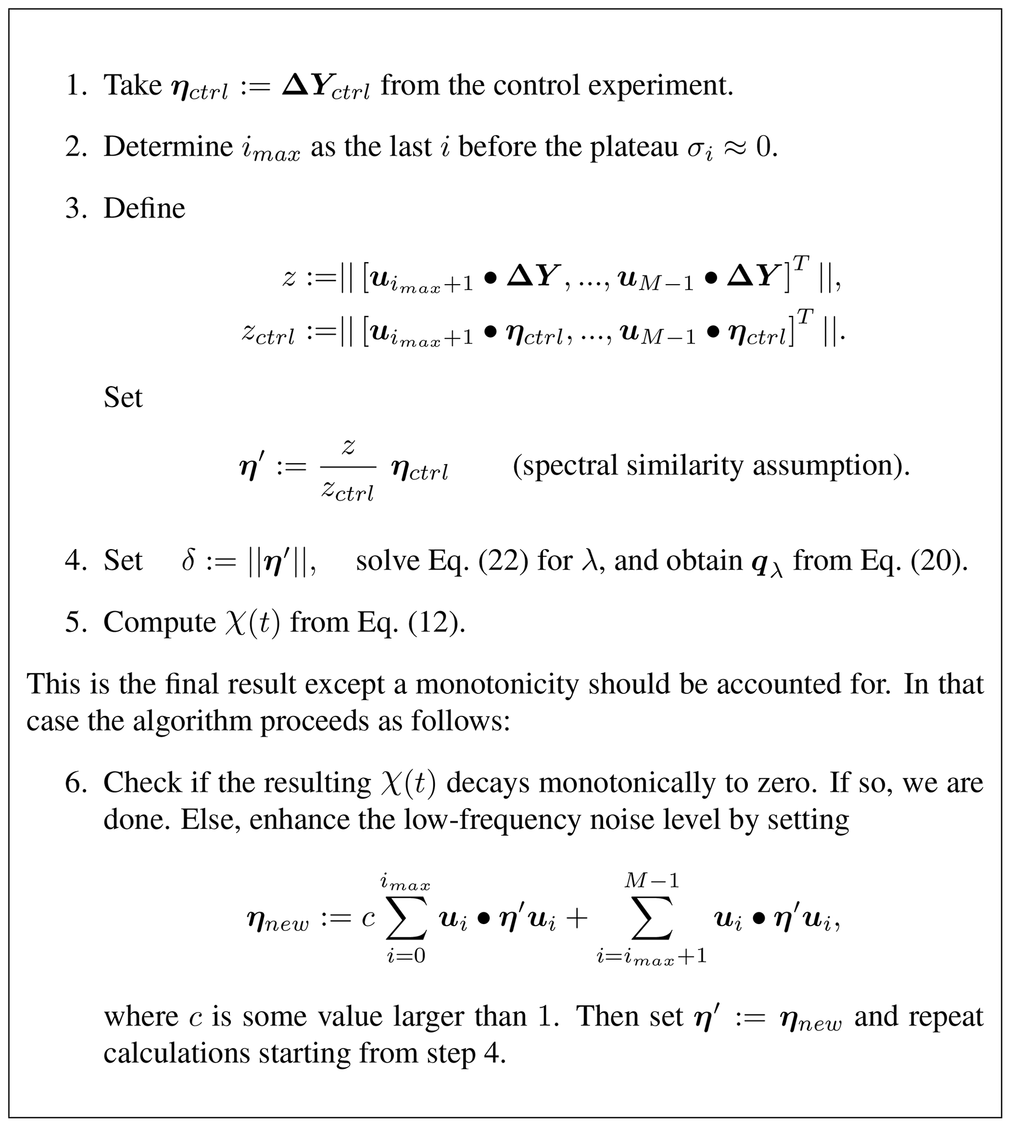
This leads to the overall algorithm listed in Fig. 1. The first five steps have already been explained at the end of Sect. 3.3.2. To account for monotonicity, the additional step 6 combined with the loop back to step 4 has to be iteratively executed. To enhance the low-frequency noise level as explained above, we calculate in step 6 a new noise vector ηnew by keeping the high-frequency part from η and enhancing its low-frequency components by a factor c>1. Then we recompute χ(t) from steps 4 and 5 and once more check for monotonicity.
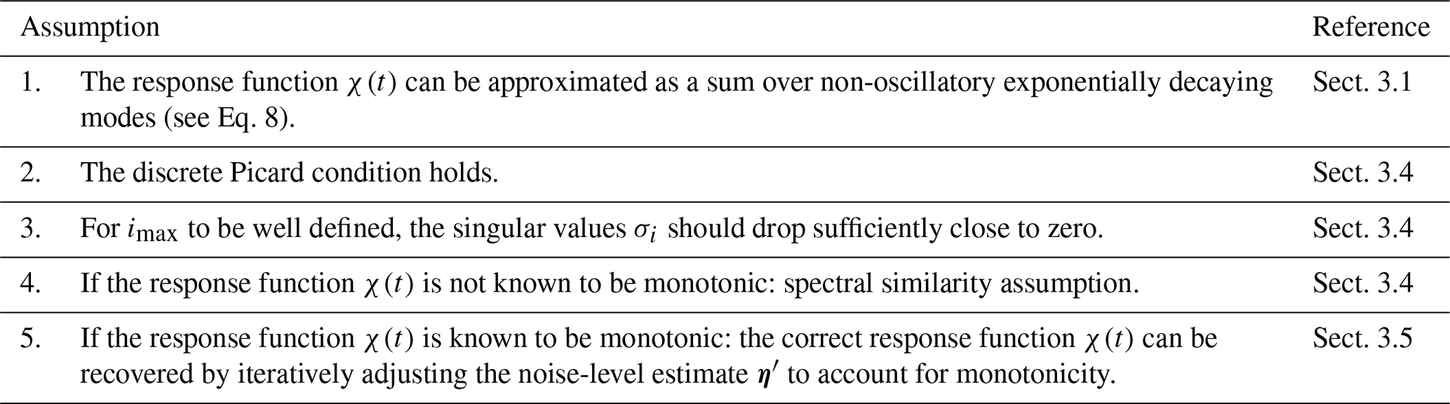
For the RFI algorithm to be applicable, two conditions must be met: (1) a linear response exists for sufficiently weak perturbation and, (2) in addition to the response experiment, a control experiment is also available. The assumptions needed for the successful application of the algorithm are summarized in Table 1.
In application to real data, the presence of noise and nonlinearities may complicate the recovery of linear response functions. Therefore, by using artificial data generated from a toy model, in the present section we analyze the robustness of the RFI method in the presence of such complications. Robustness for real data is studied in Part 2.
4.1 Toy model and artificial experiments
As a toy model we take
Here the matrix describes the relaxation of the unperturbed model. The second right-hand-side term represents the deterministic forcing constructed from the time-dependent forcing strength and the coupling vector a∈ℝD. Additionally, the system is perturbed by the stochastic forcing , which for simplicity is assumed to be white noise. To make the relation to the carbon cycle considered in Part 2, the components of x may be understood as the carbon stored in plant tissues and soils at the different locations worldwide, so that the observable is the analog of globally stored land carbon. The solution of the system is
We assume from the outset M to be diagonal with eigenvalues , the being the relaxation timescales. Then
with the linear response function χ*(t) and the noise term η*(t) given by
To complete the description of the toy model, one has to specify its parameters. For the dimension D we take 70, and the timescales are assumed to be distributed logarithmically between and , i.e., with . With carbon cycle applications in mind, the distribution of the components of the coupling vector is adapted from the log-normal rate distribution found by Forney and Rothman (2012) for the decomposition of soils:
with μ and σ chosen so that the peak timescale is around τ=5 and the limits of the log-normal distribution are approximately within τ=0.1 and τ=200 (see the “true” spectrum in Fig. 3). The components of n are taken as uncorrelated, i.e., 〈ni(0)nj(t)〉=ξδijδ(t), with standard deviation ξ being chosen differently in different experiments.
Table 2Experiments considered in this study. Forcings are shown in Fig. 2. To standardize the types of experiments considered here and in Part 2, we select forcing functions that mimic those employed in climate change simulation experiments to whose data the RFI method is applied in Part 2. Note that in principle any type of forcing could be employed.
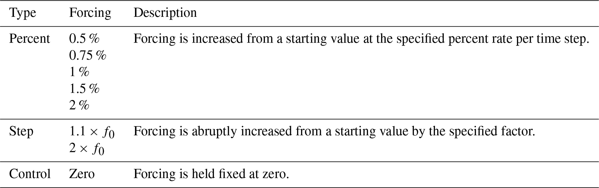
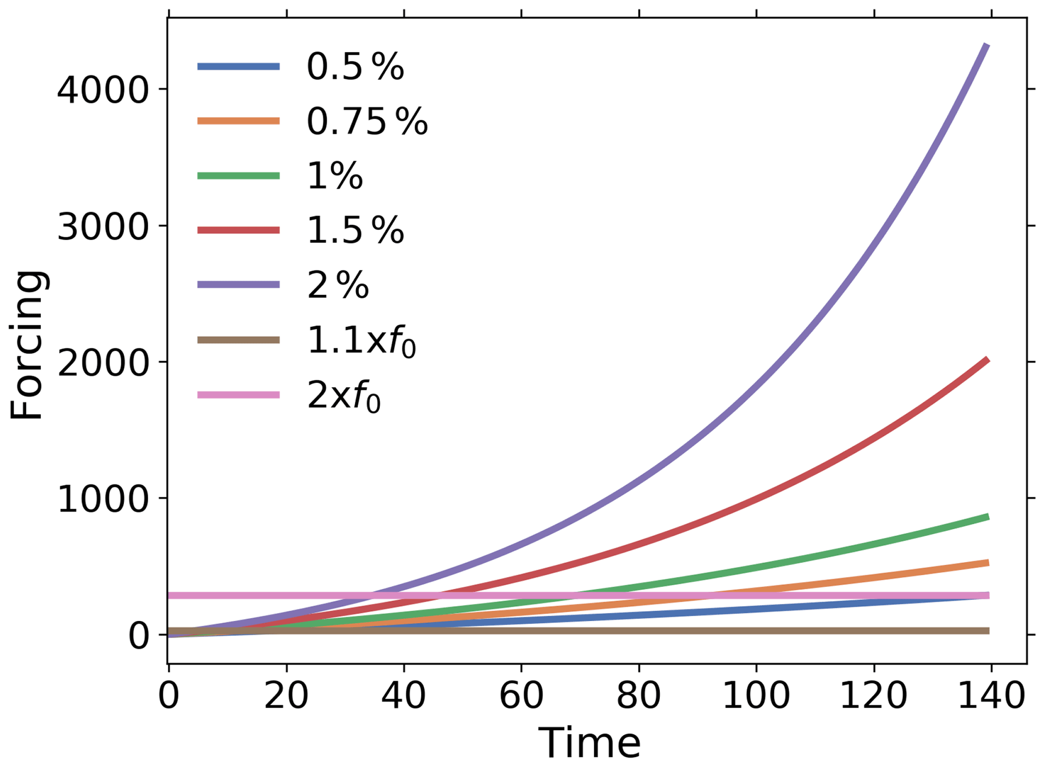
Figure 2Forcings for the experiments considered in this study. To standardize the type of experiments considered here and in Part 2, we select forcing functions that mimic those employed in climate change simulation experiments to whose data the RFI method is applied in Part 2. Note that in principle any type of forcing could be employed.
In our experiments we explore how Y(t) behaves as a function of the forcing f(t). To this end, we choose a forcing function f(t) (see Table 2 and Fig. 2). The most obvious way to perform the toy model experiments would be to integrate Eq. (30). However, to have better control over the noise, it is for our purpose more appropriate to use the analytical solution (Eqs. 32–34). Hence, we numerically integrate Eq. (32), using the representation Eqs. (33) and (34). The data from these experiments are then used to investigate the performance of the RFI algorithm to recover χ*(t). Since all ai values are non-negative, the response function (Eq. 33) is monotonic, so that we apply the extended version of the algorithm (see Fig. 1, including step 6). In all experiments we generate N=140 data points to have a time series of similar length to the climate change simulations analyzed in Part 2 (140 years, one value for each year). To apply the RFI method, the noise from an associated control experiment is also needed. This is obtained from Eq. (34) by using another realization ni(t) of white noise for each system dimension i.
4.2 Choice of parameters for the RFI method
To apply the RFI method, we choose M=30 timescales for the recovery of χ*. Using and , we distribute the spectrum of timescales according to Eq. (10). These parameters are also used for the application on the carbon cycle in Part 2 and for the comparison with previous methods in Sect. 5.
4.3 Ideal conditions
To gain trust in the numerics of our implementation of the RFI method, we present in this section a technical test considering conditions under which it is known that the linear response function should be quite perfectly recoverable. Such ideal conditions are characterized by perfect linearity and absence of noise. Hence we use the presented toy model (which is anyway linear) in the absence of noise (n=0) for this test. Actually, this will not be a full test of the algorithm but only of the implementation of its basic apparatus (Sects. 3.2 and 3.3.1), culminating in Eq. (20) since in the absence of noise, the method to determine the regularization parameter λ (Sects. 3.3.2 and 3.5) is not applicable. One might think that in the absence of noise one could use Eq. (19) to determine the linear response function, but even under such ideal conditions the ill-posedness of the problem calls for regularization to suppress the numerical noise that prevents one from obtaining a sensible solution from Eq. (19) (see the discussion in the paragraph after Eq. 19). However, choosing the small value of for the regularization parameter when evaluating Eq. (20) is sufficient for this technical test.
Figure 3c shows the response of the noiseless toy model to the forcings shown in Fig. 2; i.e., we performed the experiments listed in Table 2, although for the present test the control experiment is not needed.
Applying Eq. (20) to the experiment data gives the spectrum qλ shown in Fig. 3a. Here, we derived the spectrum qλ for each experiment separately, although in the figure only single dots are seen, because all results coincide so closely and are almost indistinguishable from the “true” solution q*, as was expected for this ideal case. The next Fig. 3b shows the response function obtained from the spectra qλ using Eq. (12). Obviously from Fig. 3a the “true” response function is reconstructed perfectly from whatever experiment is used. As a final test we predict using in Eq. (1) the response function obtained from the 1 % experiment the responses of other experiments, and indeed, these predicted responses are indistinguishable from the responses obtained directly from the experiments (see Fig. 3c). This latter result demonstrates perfect robustness of the numerical approach to recover the responses in this ideal case.
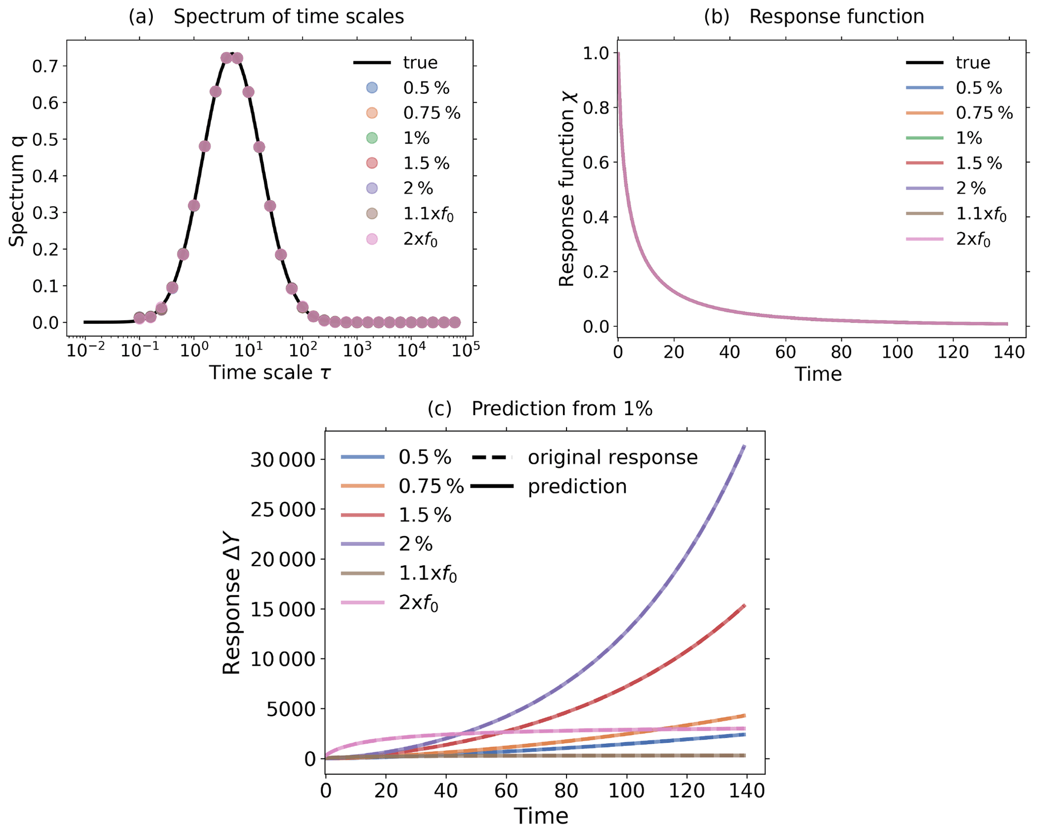
Figure 3Demonstration of robust recovery for noise-free data from the toy model: (a) recovered qλ; (b) recovered χ(t); and (c) original responses and predictions using χ(t) derived from the 1 % experiment. Reconstructed values are almost indistinguishable from original data. To plot the “true” spectrum of the toy model in subfigure (a), we used the relation , which can be obtained by comparing Eq. (33) with Eq. (12). Since from the discrete spectrum the response function and the response may be obtained for any time t, the spectrum is plotted as dots, while the response function and response are plotted as continuous lines. The regularization parameter is chosen as .
4.4 First complication: noise
The presence of noise may severely hinder the detailed recovery of χ*(t) due to the ill-posed nature of the problem. In order to demonstrate the effect of the addition of noise on the quality of the derived χ(t), we define a relative error for the prediction of the responses from different experiments. Consider a particular experiment – which is in our case the 1 % experiment – from which we have obtained by the RFI method the response function, which we call here χ0(t). The relative error for the prediction of the response from an experiment “k” by the recovered χ0(t) via the convolution (Eq. 1) is
where ⋆ stands for the discrete form of the convolution operation (Eq. 1) used to predict the responses, i.e., . In the following we denote as the prediction error for the experiment “k”. To measure the quality of the prediction across multiple experiments, we also define the mean prediction error
where K is the number of predicted responses. The reader may wonder why we quantify the quality of the recovery only indirectly from the responses found in different experiments and not directly from the recovery of χ(t). The reason is that in real applications the “true” χ(t) is not known but the responses are. The reliability of this indirect measure for the quality of the recovery is discussed in Sect. 5.
To study how the quality of the recovery depends on the noise level, we introduce the signal-to-noise ratio (SNR) of the response data from a perturbation experiment as
where δ is the final noise-level estimate obtained by the RFI method, as described in Sect. 3.3.2 (see Eq. 29).
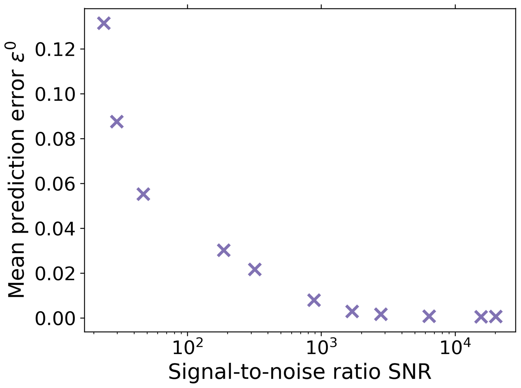
To demonstrate the dependence of the mean prediction error (Eq. 37) on the SNR, we performed 1 % experiments using different noise levels. The resulting dependence is shown in Fig. 4. As expected, for a small error a sufficiently large SNR is needed; i.e., a good recovery may be hindered by a too high noise level.
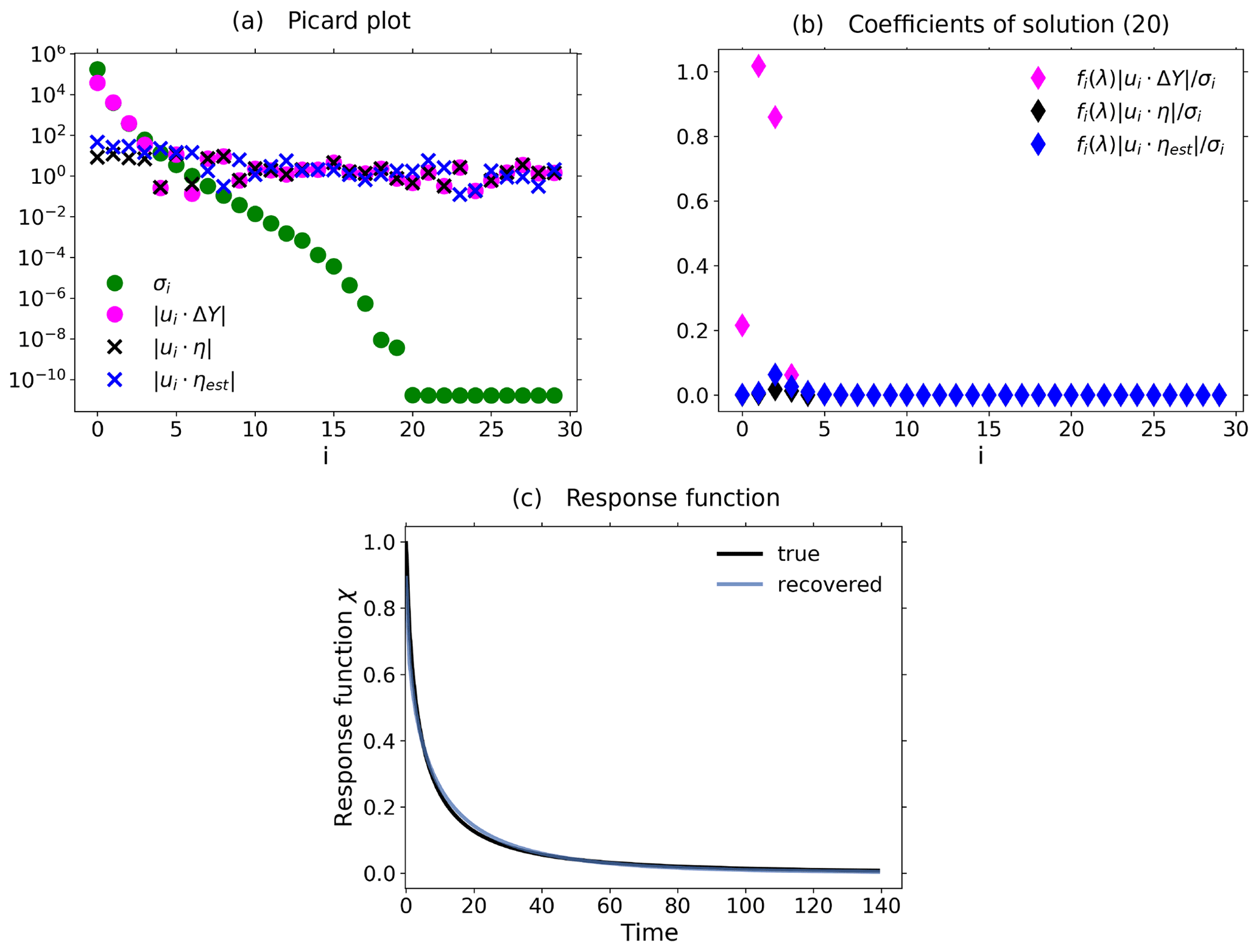
Figure 5Demonstration of the operation of the RFI algorithm in the presence of noise using toy model data from a 1 % and control experiment. To demonstrate the relevance of the noise-level adjustment (step 3 from Fig. 1), the standard deviation of the noise in the control experiment was taken to be 10 times smaller than that for the noise in the perturbed experiment. (a) Picard plot showing the singular values σi and the projection coefficients of the data , the “true” noise , and the final noise estimate ; (b) coefficients of the regularized solution (Eq. 20); (c) “true” and recovered linear response functions. Since the RFI algorithm correctly adjusted the noise level to the “true” noise in the data, the resulting regularized solution has contributions only from the first few projection coefficients which are not completely obscured by noise. Overall, the recovery is almost perfect, because the SNR (chosen as about 520) is still sufficiently good and because the noise was chosen to conform with the spectral similarity assumption. The regularization parameter determined by the algorithm is λ≈ 30 364. Because the noise-level adjustment (step 3 from Fig. 1) already gave a good estimate of the “true” noise in the data, no monotonicity check was needed (step 6 from Fig. 1).
In Fig. 5 we demonstrate how the overall noise-level adjustment in step 3 of the RFI algorithm (see Fig. 1) affects regularization to recover the correct response function. To guarantee that the overall level of the noise spectrum is indeed substantially different in the control and perturbed experiments (so that the adjustment is really needed), we take for the noise in the control experiment a standard deviation 10 times smaller than that for the noise in the perturbed experiment. To demonstrate how the adjustment works, it is helpful to consider the so-called “Picard plot”. This type of plot was originally introduced to analyze the spectral characteristics of an ill-posed problem (see, e.g., Hansen, 1992). In Fig. 5a we show the Picard plot for data obtained from a 1 % experiment with the toy model using a SNR of ≈ 520 to ensure a good recovery. The singular values σi decrease to extremely small values as the index i increases. This demonstrates that the problem of solving for the response function is indeed ill-posed and therefore regularization is needed for its solution (compare Eq. 19 with Eq. 20). The data labeled by are the “true” noise coefficients, obtained by subtracting the “clean” response Aq, known analytically from the toy model description, from the noisy toy model response ΔY. Comparing them to the projection coefficients of the response , one sees that with the exception of the first few coefficients the response is dominated by its noise content. Accordingly, only the information contained in these first few coefficients is recoverable from this ill-posed problem whatever method is used. The data labeled by have been added to the Picard plot to demonstrate how the RFI algorithm operates: these data are the projection coefficients of the estimated noise content in the data, where ηest is the final value of η′ obtained by the RFI method. Obviously, the RFI algorithm correctly estimates the “true” noise level not only at high frequencies – where it is correct by the noise-level adjustment in step 3 of the RFI algorithm (see Fig. 1) – but also at low frequencies, where it is predicted from the adjusted low-frequency components of the control experiment (also step 3). Accordingly, in this case the spectral similarity assumption holds, and there is no need to further adjust the noise level (step 6).
How the estimation of the noise in the data and the resulting regularization affects the projection coefficients of the spectrum q can be seen in Fig. 5b: only those few coefficients not dominated by noise contribute to the regularized solution. In this case these few coefficients selected by determining the regularization parameter λ from the noise level are sufficient for an almost perfect recovery of the response function, as seen in Fig. 5c.
It is important to note that in the situation of Fig. 5, where the overall noise level differs considerably in the control and perturbed experiments, a naive noise estimate taken from the control experiment without the adjustment in step 3 (as first suggested in Sect. 3.3.2) would severely underestimate the noise actually in the data. This would in turn lead to an underestimation of the regularization parameter (see Groetsch, 1984, Theorem 3.3.1). As a result, the wrong filtering by regularization would leave projection coefficients dominated by noise in the solution, likely leading to large errors in the recovered response function. This example therefore demonstrates the relevance of the noise adjustment in step 3.

Figure 6Demonstration of the additional noise-level adjustment in the presence of a monotonicity constraint using toy model data from a 1 % and control experiment: (a) Picard plot; (b) coefficients of the regularized solution (Eq. 20) and (c) recovered linear response function. All the figures are based on the same toy model experiments using a SNR = 1189. To demonstrate the effect of the noise-level adjustment, the spectral similarity assumption is broken by artificially increasing the low-frequency components of the noise in the experiments. The plots in the first row show the results from the RFI algorithm in the absence of additional noise-level adjustment (step 6 in Fig. 1). Although the “true” response function of the toy model is monotonic, the response function recovered by the RFI algorithm is non-monotonic (last figure in the first row). However, if the noise adjustment is switched on (second row), the response function is correctly recovered as monotonic (last figure in the second row). Arrows in subfigures (b) indicate the index icritical that separates components of the solution that are only weakly suppressed (i<icritical) from those that are almost completely suppressed (i≥icritical). The regularization parameter determined by the algorithm is λ≈1 for the first row and λ≈ 11 450 for the second. For more details, see the text.
Finally in this section, we demonstrate that by accounting for monotonicity of the linear response function, one may obtain a better estimate of the low-frequency components of the noise whereby the recovery of the response function is improved. In Fig. 6 we plot results from toy model experiments where the spectral similarity assumption does not hold. This was achieved by artificially enhancing the low-frequency components of the noise η*(t) in Eq. (32). The top row plots show the results from the recovery when the additional noise-level adjustment was not used. Because the spectral similarity assumption does not hold, the estimated low-frequency components of the noise do not match those of the “true” noise (Fig. 6a1). Ideally, only those four projection coefficients of the data which are larger than the projection coefficients of the “true” noise should contribute to the recovered response function. Instead, as seen in Fig. 6b1, the coefficients with indexes between i=4 and i=7 give the dominant contributions because they are larger than the estimated noise coefficients (compare Fig. 6a1). Therefore, the recovery of the response function is poor (Fig. 6c1). However, since in this case the low-frequency components of noise are such that the recovered response function is non-monotonic although the “true” response function is known to be monotonic, one may further adjust the noise level to improve the results.
This further adjustment is the purpose of step 6 of the RFI algorithm (see Fig. 1). Its effect is demonstrated by the second-row plots of Fig. 6: the estimated noise components now match the “true” noise components better that had been underestimated in the first row (compare Fig. 6a2 and a1), so that only those four components that carry information (compare in Fig. 6a2 the projections for low index i with ) survive the regularization (Fig. 6b2). As a result, the quality of the recovery of the response function has considerably improved (Fig. 6c2).
4.5 Second complication: nonlinearity
The second difficulty in recovering the linear response function χ(t) from a perturbation experiment may arise from nonlinearities present in the considered system. Generally it must be suspected that nonlinearities are present, so that they should not hurt as long as they are small, and indeed, from the viewpoint of regularization, contributions from nonlinearities can be considered an additional noise, so that in principle they can also be filtered out. However, as with noise, when getting stronger they cause a deterioration of the recovery of the response function. In the following, we show this more formally and discuss in detail how the RFI algorithm behaves in the presence of nonlinearities.
To understand how contributions from nonlinearities affect the recovery of the response function, we write the nonlinear terms in Eq. (5) collectively as . This formally gives
instead of Eq. (13). Plugging this into Eq. (20), the spectrum is obtained as
Accordingly, the nonlinear contributions can be understood as an additional noise in the spectrum qλ, so that the theory of regularization fully applies when replacing η by the combined noise . Hence, as in their absence, nonlinearities do not prevent the application of regularization as long as the signal is not buried under this combined noise.
However, for the RFI algorithm to give good results, a second condition is that the contributions from must not be large compared to those from η. To understand this, one must realize that the response and with it the nonlinear contributions are dominated by low-frequency components because of the low-frequency nature of the forcing for the problems of interest (for instance in % experiments). The RFI algorithm uses an estimate for the noise level in the perturbation experiment obtained from the control experiment assuming that the spectral distribution is approximately the same in the noise from the control experiment and the noise in the data from the perturbation experiment (spectral similarity assumption; step 3 of Fig. 1). However, the control experiment does not contain any contributions from nonlinearities because the forcing is zero. Therefore, if in the data from the perturbation experiment the contributions from nonlinearities are not small compared to those from η, the spectral similarity assumption does not hold. Since this assumption is at the heart of the RFI algorithm, its breakdown leads to a poor recovery of the linear response function.
All this is demonstrated in the following by toy model experiments. For this purpose, we artificially consider the response of the toy model not in Y but in its nonlinear transform
where the parameter a determines the strength of the nonlinearity. The particular functional form chosen for Ynonlin(t) mimics the nonlinear effect of saturation encountered for instance in the land carbon sink when atmospheric CO2 rises to high values. In the following, to demonstrate the effect of nonlinearities, we set the noise level in the toy model experiments to a rather small value in order to have a good SNR in the experiments considered.
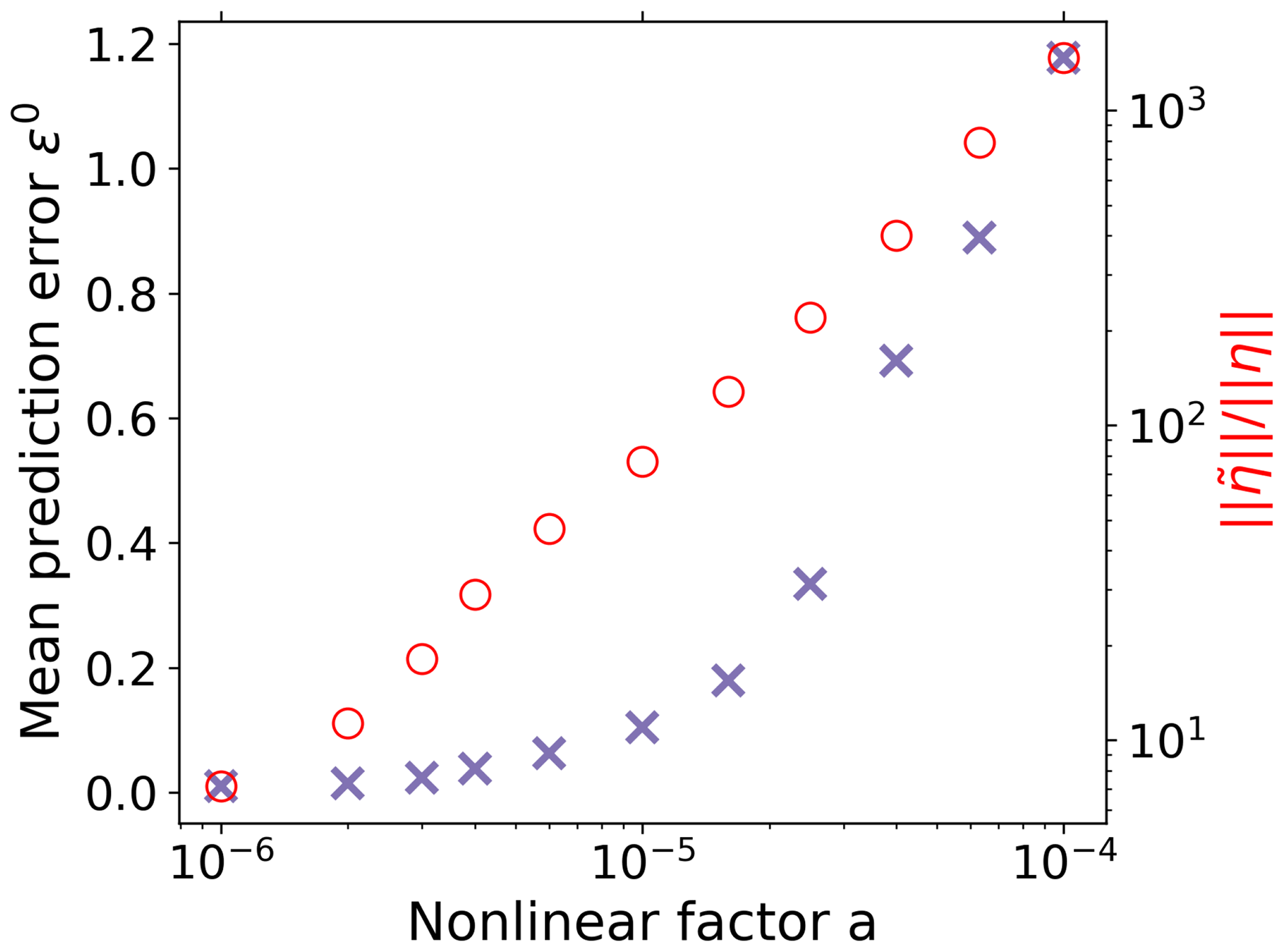
Figure 7Mean prediction error (Eq. 37) of the recovery when deriving χ(t) for different values of the nonlinearity factor a of the toy model. As a increases, the recovery of χ(t) deteriorates because the level of the contributions from nonlinearities becomes large compared to the noise level ; how these terms are computed for the toy model is explained in Appendix D. To demonstrate here the pure effect from the breakdown of the spectral similarity assumption, the RFI algorithm is used here without the additional noise-level adjustment enforcing monotonicity.
In Fig. 7 we show by plotting the mean prediction error (see Eq. 37) how the recovery of the response function deteriorates as the nonlinearity parameter a increases. To demonstrate that this is indeed caused by a breakdown of the spectral similarity assumption, we plot in addition the ratio . It is seen that, indeed, as claimed above, the recovery works well only when this ratio is not large, i.e., when the contributions from nonlinearities are not large compared to those from the noise η.
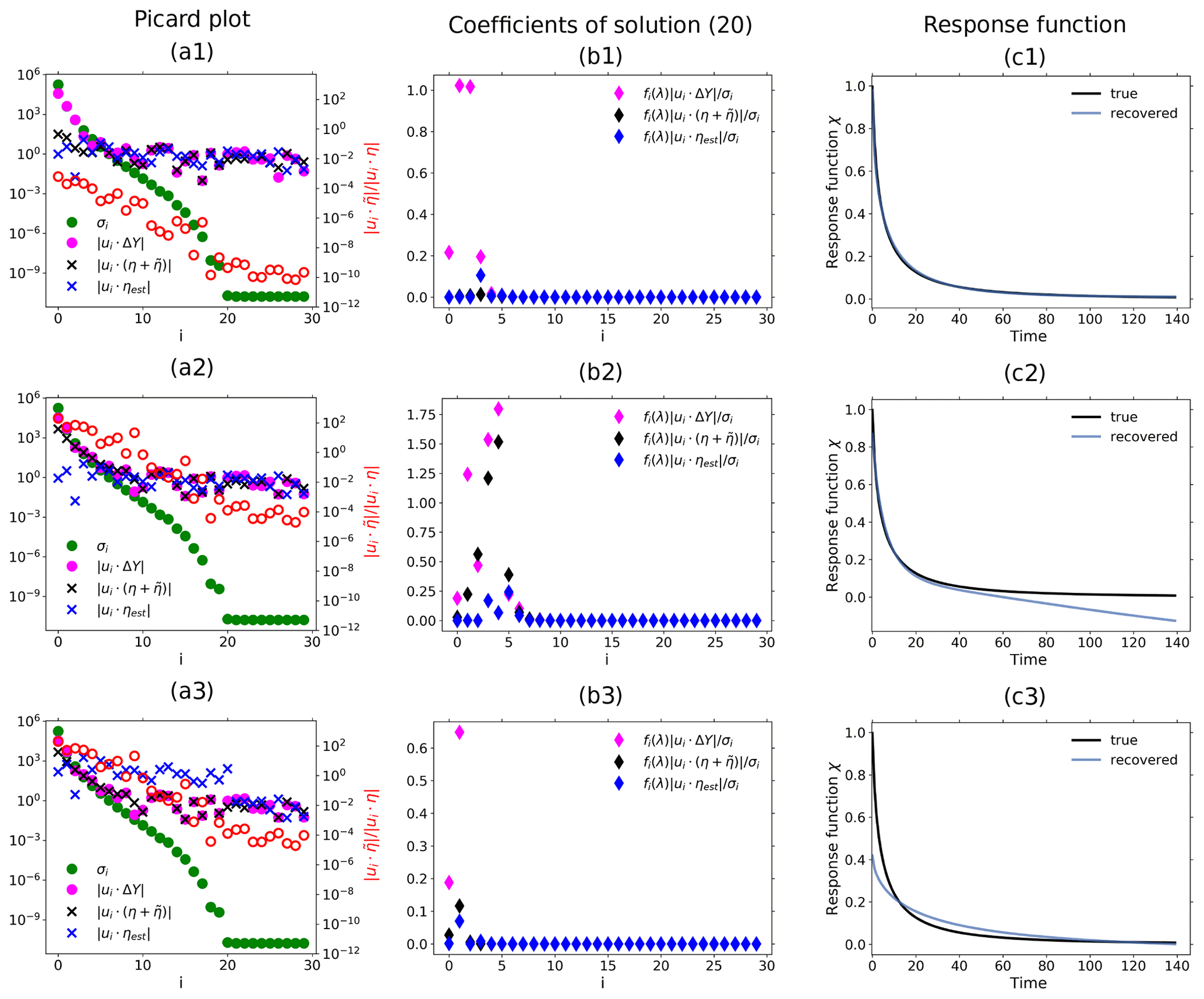
Figure 8Demonstration of how nonlinearities affect the recovery of the response function: (a) Picard plot; (b) coefficients of regularized solution (Eq. 20) and (c) recovered linear response function. First row: nonlinearity factor (no monotonicity check); second row: nonlinearity factor (no monotonicity check); third row: nonlinearity factor (with monotonicity check). The noise is overestimated in the low-frequency spectrum in the third row because nonlinearities yield a derived χ(t) that does not obey the monotonicity constraint. As a consequence, the method increases the level of low-frequency components until the monotonicity constraint is obeyed. The failure to obey the monotonicity constraint and consequent large overestimation of noise in this case can be taken as an indication of the presence of nonlinearities in the response. Note that the “true” linear response function in this nonlinear case a≠0 is obtained analytically from the linear case a=0 via Eq. (41) (see Appendix D). The regularization parameter determined by the algorithm is λ≈3120 for the first row, λ≈74 for the second, and λ≈14 611 873 for the third. For more details, see the text.
More insight into how nonlinearities affect the recovery is obtained from the more detailed SVD analysis shown in Fig. 8. The first row of subfigures was obtained from the toy model assuming a rather small nonlinearity (). In the Picard plot (Fig. 8a1) it is seen that in this case both conditions necessary for a good recovery are met: first, the signal is clearly visible above the combined noise (see the first four components). Second, in this case is small over the whole spectrum; i.e., the contributions from are small compared to those from η. As explained above, because this second condition is also met, the noise estimate from the RFI algorithm ηest is a good approximation to the combined noise across all frequencies (compare in the Picard plot to ). As a result, the four components selected by the regularization for the recovered solution (Fig. 8b1) are precisely those dominated by the signal (compare with ). This example demonstrates that as long as these two conditions are met, small contributions from nonlinearities do not prevent a good recovery of the response function (see Fig. 8c1).
In the second row of Fig. 8, we demonstrate how the violation of the second condition obstructs the recovery. In this case the nonlinearity parameter has been given a larger value (). As a consequence, one sees in the Picard plot that the low-frequency components of the combined noise are enhanced. The first condition is still met: the signal is visible above the combined noise (see the first two components). However, now the ratio becomes large at low frequencies, violating the second condition. As explained, the violation of the second condition leads to the breakdown of the spectral similarity assumption. As a result, the RFI algorithm underestimates the combined noise at low frequencies (compare in the Picard plot to ). Using this wrong noise estimate, regularization selects components for the recovered solution that are to a large extent dominated by the combined noise (see components i=2 to i=6 in Fig. 8b2). The result is that the strong low-frequency contributions from nonlinearities deteriorate the recovery of the response function at long timescales (Fig. 8c2).
In the third row, we demonstrate for this type of nonlinearity that by accounting for monotonicity one can remove from the recovered solution all components dominated by noise. For this purpose, we set the nonlinearity parameter to the same value as for the second row () but employ the additional noise-level adjustment (step 6 of Fig. 1); i.e., the low-frequency range of the noise estimate is now automatically adjusted in order to recover a response function that decays monotonically to zero. As seen in the Picard plot, the additional noise-level adjustment results in an artificial enhancement of the low-frequency components of the noise estimate, with a large jump separating the low- from high-frequency ranges. In this case, such enhancement is able to better estimate the largest components of the combined noise (first few components in the Picard plot). As a consequence, regularization correctly selects for the recovered solution only the two first components which are not dominated by noise (Fig. 8b3). Unfortunately, as seen in Fig. 8c3, these two first components do not contain enough information for a perfect recovery, since the quality improves at long timescales but deteriorates at short timescales (compare Fig. 8c3 and c2). This is a consequence of how regularization works: it filters out components dominated by noise (or in this case nonlinearity) at the expense of also removing useful information contained in those components.
As a last test of the quality of the results given by the RFI method in application to the toy model, in this section we compare our method against two existent methods in the literature to identify response functions in the time domain. The comparison is performed for the particular case where the response function is known to be monotonic and also for the more general case where it is not. As a side issue, this section also reveals some insight into the relation between the quality of the recovery of χ(t) as measured by the prediction of responses and the quality of the recovery of χ(t) itself.
In climate science, the most commonly used method is to obtain χ(t) from an impulse response, i.e., the response to a perturbation of Dirac delta type (e.g., Siegenthaler and Oeschger, 1978; Maier-Reimer and Hasselmann, 1987; Joos and Bruno, 1996; Joos et al., 1996; Thompson and Randerson, 1999; Joos et al., 2013). Here we call it the pulse method. Although this method is conceptually straightforward, in some cases it might not yield satisfactory results. Since the perturbation is only one “pulse”, depending on the observable of interest it may give a response with a small SNR. As a consequence, the recovered response function may be severely affected by noise. On the other hand, if the strength of the pulse is made large to obtain a good SNR, the linear regime may be exceeded. In this case, the impulse response does not correspond anymore to the linear response function.
The second method consists of deriving the linear response function from a step response, i.e., the response to a Heaviside-type perturbation (e.g., Hasselmann et al., 1993; Ragone et al., 2016; MacMartin and Kravitz, 2016; Lucarini et al., 2017; Van Zalinge et al., 2017; Aengenheyster et al., 2018). Here we call it the step method. Due to the special form of this “step” perturbation, the linear response function can in principle be derived from
where fstep is the step perturbation and ΔYstep is the corresponding response. Unfortunately, such derivation involves numerical differentiation, which is known to be an ill-posed problem (Anderssen and Bloomfield, 1974; Engl et al., 1996). Because the problem is ill-posed, noise is amplified, potentially resulting in large errors in the derived linear response function.
These two methods therefore share two limitations: first, they require a special perturbation experiment; second, because of noise in the data they might yield a response function with large errors. In principle, the second limitation may be overcome by using instead of a single response the ensemble average over multiple responses. However, this comes at the expense of the numerical burden of performing multiple experiments, which is especially large when dealing with complex models such as state-of-the-art Earth system models.
The main advantages of the RFI method lie precisely in overcoming these two limitations: it recovers the response function from any type of perturbation experiment and automatically filters out the noise by regularization.
For the results of this section, we performed ensembles of 200 simulation experiments with the toy model (see Sect. 4.1). Each ensemble member is defined by a realization of the noise η*(t) with a fixed standard deviation (see Eq. 34). Each realization was added via Eq. (32) to three experiments: 1 %, step (2×f0), and pulse (4×f0). Note that because of the issue with the SNR mentioned above, we had to employ for the pulse experiment twice the forcing strength employed for the step experiment. Further, for each ensemble member an additional realization of the noise was generated to serve as a control experiment to compute the noise estimate for the RFI method (step 1 of Fig. 1).
We computed the response function by the pulse and step method as follows. For a pulse experiment the forcing is f(t)=aδ(t) with forcing strength a, so that the response is given by
Therefore, for the pulse method we took the response from the pulse experiment and obtained the response function by
The recovery by the step method was calculated by taking the response from the step experiment and applying Eq. (42). The derivative was computed by forward difference.
To obtain comparable results with these two methods, we recovered the response function by the RFI method from the same pulse and step experiments. To compare the quality of the results using also an experiment not decidedly tailored for the identification, we include additionally the recovery from the 1 % experiment.
To obtain a quantitative comparison for the quality of the recovery for each method, we define the recovery error:
where χ is the recovered response function and χ* is the “true” response function, which is known because we use the toy model. In contrast to the prediction error that measures the quality of the recovery of χ(t) by means of the response (see Eq. 45), the recovery error εr measures the quality of the recovery of χ(t) itself. Another reason for introducing the recovery error is to compare its results with results from the prediction error. By doing that, we can gain insight into how much the prediction error can be trusted as an indirect measure of the quality of recovery in real applications, where the “true” response function is not known.
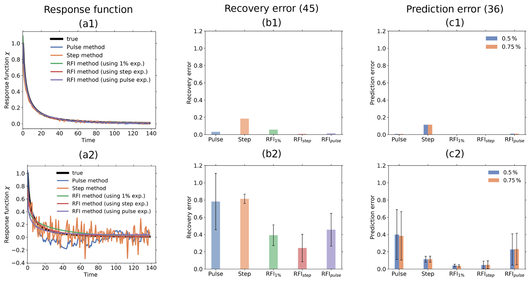
Figure 9Quality of response function recovery by the full RFI method (including step 6 in Fig. 1) in comparison to the pulse and step method. Subscripts at “RFI” indicate the experiment from which the response function was recovered with the RFI method. First row: taking the average over the whole ensemble of toy model experiments for recovery; second row: performing the recovery for each ensemble member separately. (a1) Recovered response function; (b1) recovery error; (c1) prediction error (Eq. 36); (a2) example of recovered response function from one ensemble member; (b2) statistics of recovery error; (c2) statistics of prediction error (Eq. 36). The prediction error is separately computed for the 0.5 % and 0.75 % experiments. Taking the ensemble average, all methods perform well (see first row). However, taking only one ensemble member, the RFI algorithm gives better recovery and prediction errors than the pulse and step methods when comparing the same responses (see second row).
First, we compare the pulse and step methods against the full RFI algorithm, i.e., the RFI algorithm taking monotonicity into account (step 6 in Fig. 1). Results are shown in Fig. 9. In the first row of subfigures, we took for the recovery the ensemble average over the 200 responses for each experiment. For the RFI method, we took the ensemble average over the control experiments as well to estimate the noise (step 1 of Fig. 1). As shown in Fig. 9a1, with this approach all the methods recover the response function almost perfectly. The quality of the recovery is quantified by the recovery error in Fig. 9b1. The RFI method shows the smallest values for the step and pulse experiments when compared to the step and pulse methods. Overall, the step method clearly shows the largest value. To quantify the quality of the prediction, we plot in Fig. 9c1 the prediction error (Eq. 36). As seen, values are even smaller than for the recovery error. Overall, we see a similar pattern: the step method again stands out, with other methods showing much smaller error values.
In the second row, we compare results by taking only a single response for the recovery. Since the quality of the recovery by the different methods may vary depending on the particular noise realization, we again performed 200 simulations to obtain better statistics but this time deriving the linear response function for each ensemble member separately. Figure 9a2 shows an example of recovery for one of the ensemble members. As expected, the recoveries by the pulse and step methods largely deviate from the true response function. For the pulse method, the large errors result from the low SNR of the pulse response: even taking twice the forcing strength of the step experiment, the SNR of the pulse response is of order 100 against order 101 for the step and 1 % responses. For the step method, on the other hand, the large errors are not a result of a low SNR but of the noise amplification associated with the ill-posedness of numerical differentiation. In contrast to the recovery by these two methods, because of regularization the recoveries by the RFI method are smoother and visually seem to better fit the true response function. To quantitatively check these results, we plot in Fig. 9b2 for each method the average and standard deviation over the 200 values of the recovery error (one for each ensemble member). The figure shows that the pulse and step methods indeed display the largest average recovery error, with the pulse method having a much larger spread. Such spread is probably related to the low SNR in the response from the pulse experiment. The results from the 1 % and pulse experiments by the RFI method are better, showing comparable error magnitudes. The smallest average recovery error is obtained from the RFI method using the step experiment. In Fig. 9c2 we show the average and standard deviation over the 200 values of the prediction error (Eq. 36). The smallest average prediction errors are obtained from the RFI method using the 1 % and step experiments. The largest errors are obtained for the pulse method and the RFI method using the pulse experiment. In contrast to the situation for the recovery error, for the prediction error no substantial difference between the two is found. Note also that when comparing recoveries from the same response (i.e., comparing “Pulse” with “RFIpulse” and “Step” with “RFIstep”), the RFI method gives better results than both the pulse and step methods. Another interesting point is that prediction errors for the step method remain approximately unchanged by taking the ensemble mean and a single response (compare “Step” in Fig. 9c1 and c2). Overall, as in the first row, the prediction error shows for each individual method values smaller than the recovery error. However, now there is a difference between the plots for the recovery and prediction error: although the pulse and step methods show the largest averages, with values of comparable size for the recovery error, for the prediction error the pulse method has the largest average, with a value much larger than the step method.
This difference can be better understood as follows (see MacMartin and Kravitz, 2016, for more details, including the influence of the forcing scenario). Because Eq. (1) is ill-posed, the convolution operator acts on χ(t) as a “low-pass filter” (see, e.g., Bertero et al., 1995; Istratov and Vyvenko, 1999). This means that high frequencies in χ(t) are suppressed by convolution and show up damped in the response ΔY(t). Hence, recoveries with large errors only at high frequencies tend to give relatively small prediction errors. Because of the low SNR, the pulse method yields a recovery of χ(t) with large errors at both high and low frequencies. Although the errors at high frequencies are damped in the prediction, errors at low frequencies are not. Hence, the large recovery error results in a large prediction error. On the other hand, because of the good SNR for the step response, the step method gives a relatively good recovery of χ(t) at low frequencies, with large errors concentrated at high frequencies. As a result, the large recovery error results in only a small prediction error. This suppression of high-frequency errors might also explain why the prediction error for the step method remains unchanged when recovering the response function from a single response instead of the ensemble average. By comparing the recovery of χ(t) by the step method in Fig. 9a1 and a2, one sees that the main difference is indeed at high frequencies (the recovery in Fig. 9a2 is quite “noisy” but follows the long-term trend). This is because the noise amplification has a larger effect on the recovery from the single response due to its larger noise level. However, since low frequencies are well recovered in both cases, the resulting prediction errors are almost the same.
Overall, the analysis of Fig. 9 suggests two main conclusions. First, as expected, the prediction error indeed gives an indication of the quality of the recovery, since good recoveries result in good predictions. However, care should be taken when judging the recovery only from the prediction error, because a good prediction does not necessarily imply a good recovery: due to the ill-posedness, Eq. (1) might damp large high-frequency recovery errors, so that they do not show up in the prediction. Nevertheless, from a good prediction error one can still infer a good recovery at low frequencies, because at these frequencies large recovery errors result in large prediction errors. Since regularization filtering leaves only low-frequency terms in the recovery, the RFI method shows in Fig. 9 small prediction errors associated with small recovery errors.
Second, by taking only a single response – and not the ensemble average – the full RFI algorithm gives on average smaller recovery and prediction errors than the pulse and step methods when comparing results obtained from the same experiment.
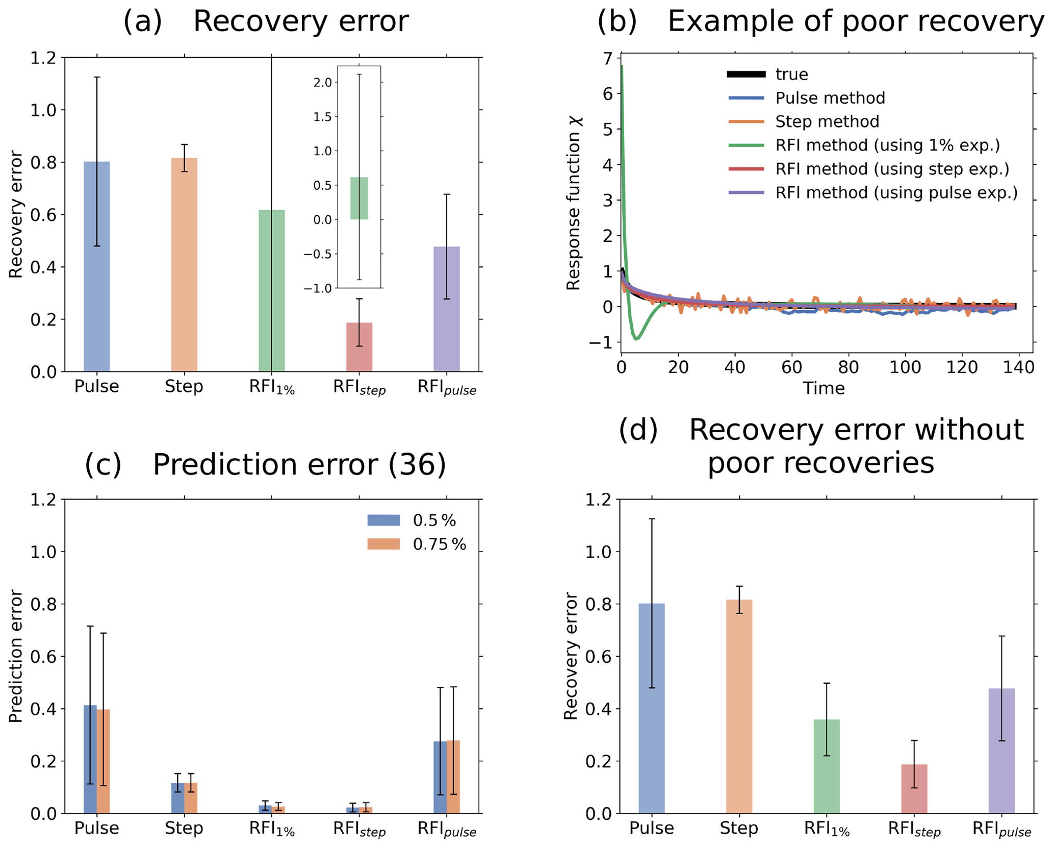
Figure 10Quality of response function recovery by our RFI method excluding step 6 in Fig. 1 in comparison to the pulse and step method. Response function is recovered taking the individual response for each ensemble member. Subscripts at “RFI” indicate the experiment from which the response function was recovered with the RFI method. (a) Statistics of the recovery error; (b) example of poor recovery with the RFI algorithm; (c) statistics of the prediction error (Eq. 36); (d) statistics of the recovery error excluding for the RFI1 % the 6.5 % of the recoveries with recovery error greater than 1. Once again, the RFI method gives better recovery and prediction errors than the pulse and step methods for the same responses. Without accounting for monotonicity, the variability in the quality of the recoveries from the 1 % experiment increases substantially, but poor recoveries are obtained in only a few cases.
However, the results above cover only the case where the full RFI algorithm is employed. In the following, we also analyze the case where monotonicity is not taken into account. For this purpose, we repeated in full detail the exercise that led to Fig. 9 but did not apply the additional noise-level adjustment to enforce monotonicity of the response function. Figure 10a shows the results for the recovery error. Once more, the RFI method gives smaller values than the step and pulse methods when comparing the recovery from the same responses. In addition, now the recovery for the RFI method using the step experiment even improved in comparison to Fig. 9b2. The reason may be related to the numerical check for monotonicity: depending on the tolerance value that is used to judge whether the recovered response function is monotonic, the additional adjustment might actually overestimate the noise level, leading to slightly worse results.
Yet the improvement brought by the additional noise-level adjustment is clear when looking at the recovery error for the 1 % experiment. Compared to Fig. 9b2, the average error increases substantially, and the spread is much larger (see inset for the whole value). As explained in Sect. 4.4, this deterioration results from cases where the noise in the response is such that the spectral similarity assumption does not hold. Since here the noise estimate resulting from this assumption is not further improved by the monotonicity check, the result is a poor recovery (see Fig. 9b for an example). However, because the large errors are mostly at high frequencies, even poor recoveries are still sufficiently good for predictions, as shown by the small mean prediction error in Fig. 9c (see “RFI1 %”). Therefore, in contrast to the case where monotonicity is taken into account, here some small prediction errors are associated with large recovery errors.
Nevertheless, we find that, although extreme, such poor recoveries are not frequent. In fact, extreme cases with recovery error εr > 1 account for 6.5 % of the recoveries. This suggests that the large deterioration in the mean and spread of the recovery error in subfigure (a) is not a result of overall poor recoveries but of only few extreme cases. To check this hypothesis, we plot in subfigure (d) the mean and standard deviation, excluding these cases from the calculations. Indeed, the result is much better, showing values comparable to the case where monotonicity is taken into account (compare “RFI1 %” in Fig. 10d and Fig. 9b2). Overall, this result indicates that at least for models of this type – where in the perturbation experiment the spectral distribution of noise does not change drastically compared to the control experiment – although monotonicity plays a role in avoiding large recovery errors, statistically most recoveries are still relatively good even without this additional improvement.
Existent methods to identify linear response functions from data require tailored perturbation experiments. Here, we developed a method to identify linear response functions from data using only information from an arbitrary perturbation experiment and a control experiment. The RFI method addresses the ill-posedness inherent to the identification problem by applying Tikhonov–Phillips regularization. The regularization parameter is computed by the discrepancy method, which involves the estimation of the noise level. For this purpose, we take advantage of information given by a spectral analysis of the perturbation experiment and by the control experiment. Assuming that the Picard condition holds, we estimate from the perturbation experiment the high-frequency components of the noise. Then, assuming that the spectral distribution of noise is approximately the same for the perturbed and control experiments (spectral similarity assumption), we estimate from the control experiment the low-frequency components of the noise. The obtained noise-level estimate can be further adjusted if the linear response function is known to be monotonic. The robustness of the method in the presence of noise and nonlinearity was demonstrated in Sect. 4. Additional sensitivity tests showing the robustness of the method under changes in the parameters for the recovery are shown in Appendix E.
As discussed in Sect. 5, the developed method to identify linear response functions is an alternative approach to existent methods in the literature, which require special perturbation experiments and often give results with large errors caused by noise. In contrast, the RFI method accounts in a systematic way for the noise and can be directly applied to data from any type of perturbation experiment once a control experiment is also given. Because it filters out the noise, its results show in the cases analyzed here a higher quality compared to results from previous methods when applied to the same data from a toy model, and because it can identify response functions from any type of perturbation experiment, the method is particularly suitable for application to data from the C4MIP carbon cycle model intercomparison as shown in Part 2 of this study.
The main novelty of the method is the estimation of the noise level (steps 1–3 of Fig. 1), which is known to be critical for the application of regularization theory. When solving a problem by regularization, the most crucial step is the computation of the regularization parameter. To compute this parameter in a way that the solution converges to the “true” solution for decreasing noise, methods need to account for the noise level (Bakushinskii, 1984; Engl et al., 1996). However, in practical applications the noise level is rarely known. Therefore, methods to obtain good estimates are needed. Our new method to estimate the noise level consists essentially of two steps: first, estimating the high-frequency components from data and then the low-frequency components from the control experiment. While the second step is completely novel, the main idea behind the first step was already brought up in earlier studies (e.g., Hansen, 1990) and has recently been further developed by methods to compute the “Picard parameter” (Taroudaki and O'Leary, 2015; Levin and Meltzer, 2017), which is different from the imax that we use in our method. The Picard parameter is computed as the index for which the components start to level off. Typically, from this index onwards the data can be interpreted as noise. For this reason, one might think that from the Picard parameter one can obtain all data components dominated by noise and thereby estimate the noise level. However, this is not generally true: for instance, if the noise has large low-frequency components such as in Fig. 8a2, then the components level off at an index larger than that at which the data start to be dominated by noise, so that in this case the Picard parameter does not determine all data components dominated by noise. In our RFI method, the interest lies in obtaining not all data components dominated by noise but only enough components to obtain the overall level of the high-frequency noise. For this purpose, we define instead of the “Picard parameter” the more conservative index imax, above which the singular values are zero and by the Picard condition the “true” data components must also be zero. In this way, we unambiguously identify data components that contain only noise (see Eq. 24). These components give the high-frequency noise level, so that in the second step the remaining low-frequency noise components can also be estimated from the control experiment (step 3 of Fig. 1).
Because our noise-level estimation is not particularly related to the problem of identifying response functions, it can in principle be applied to solve also other types of linear ill-posed problems (see, e.g., Engl et al., 1996). In general, all one needs for the application are the following.
-
A problem of the type
where given the matrix A and the noisy data y one is interested in finding x.
-
Data from a situation similar to the control experiment, where Ax=0, so that the resulting yctrl gives the noise term
-
The singular values of A decaying to values sufficiently close to zero to obtain imax.
Then, as long as both the Picard condition and the spectral similarity assumption hold, the method gives a reasonable noise estimate – since then, by assumption, the noise estimate is simply a scaling of the noise in the control experiment (see Sect. 3.3.2) – by which the regularization parameter can be determined.
While the Picard condition is necessary for a solution to be recoverable from an ill-posed problem, the validity of the spectral similarity assumption is less clear. An intuitive explanation for this assumption can be thought as follows. Since here the interest lies in identifying linear response functions, the perturbation to the system must be sufficiently weak so that the response can be considered linear. If the noise in the control experiment depends on the perturbation, a sufficiently weak perturbation will modify its characteristics only slightly. The RFI method accounts partially for this change by adjusting the overall level by which the noise increases. Nevertheless, it assumes that since the characteristics of the noise change only slightly, then the spectral components of the noise in the perturbed experiment can be thought of as having the same relative contributions as those in the control experiment. When in addition the response function is known to be monotonic, the estimate of the noise can be further improved (step 6 of Fig. 1), this time by adjusting the relative contribution of the spectral components: since the high-frequency region is known from the spectral analysis of the response, then the components of the noise are adjusted in the low-frequency region; this is done iteratively until the resulting response function becomes monotonic. Such additional adjustment has been demonstrated to give good results in the applications in the present study and subsequent Part 2 for the special case where the response function can be considered monotonic.
Although it is assumed that χ(t) is given by the spectral form (Eq. 8), this is not essential for our method. In principle, any functional form can be assumed for χ(t), or even none – in which case one would recover χ(t) pointwise. However, compared to the simpler pointwise recovery of χ(t), assuming Eq. (8) has some advantages. The most obvious is that in contrast to the pointwise approach, with Eq. (8) both χ(t) and the spectrum can be recovered together. If χ(t) is recovered pointwise, the spectrum has to be derived in a second step from χ(t), which is also an ill-posed problem (Istratov and Vyvenko, 1999). Further, the description (Eq. 8) restricts the function space for the recovered χ(t), forcing as is expected for most problems of interest, which greatly simplifies the problem compared to the case where χ(t) can assume any form. Our ansatz (Eq. 8) also has advantages in comparison with the typical multi-exponential ansatz (Eq. 7) assumed in most previous studies (see discussion in Sect. 3.1). When assuming that χ(t) is given by a sum of few exponents, an important problem is how to choose the number of exponents. The typical methods to choose this number rely on “quality-of-fit” criteria, but for ill-posed problems these criteria can be unreliable because in these problems a good fit does not mean that the derived parameters are close to the “true” parameters (see, e.g., the famous example from Lanczos, 1956, p. 272). In our approach, as long as the distribution of timescales is appropriately prescribed and the data quality is sufficiently good, numerical results indicate that the solution is approximately independent of the number of exponents (Appendix E). Moreover, compared to the multi-exponential approach, our ansatz (Eq. 8) has two additional advantages: the first is that it leads to the linear problem of finding only the spectrum q(τ) – in contrast to the nonlinear problem of finding both the timescales τi and the weights gi from Eq. (7) – which permits an analytical solution and thereby gives more transparency to the method. The second is that compared to the assumption of only a few timescales, the ansatz of a continuous spectrum of timescales is typically more realistic for real systems, which is, e.g., the case for the carbon cycle study presented in Part 2. One limitation is however that our ansatz (Eq. 8) restricts the solution to systems with exponentially relaxing responses and vanishing oscillatory contributions.
In the present paper the robustness of our method has been investigated only for artificial data taken from toy model experiments. In this analysis, we not only knew the “true” response function underlying the data, but also had control over the two complications that may hinder its recovery, namely the level of background noise and nonlinearities. Under these ideal conditions, we could carefully examine the quality of the response functions identified by our RFI method. Nevertheless, such conditions are hardly met in practice. Therefore, the applicability of our method must be investigated as well for real problems. Such an investigation is presented in Part 2 of this study.
In this Appendix we show that Eqs. (1), (7), and (1) with χ(t) given by Eq. (7) are indeed special cases of the Fredholm equation of the first kind, as claimed in Sects. 3.1 and 3.2. Since inverse problems in the form of this equation are well known to be ill-posed (e.g., Groetsch, 1984; Bertero, 1989; Hansen, 2010), this clarifies the inherent difficulties in identifying linear response functions from perturbation experiment data.
A Fredholm equation of the first kind is an equation of the type (Groetsch, 1984)
Clearly, by setting a:=0, , and , one obtains the form of Eq. (1) – which can also be seen as a Volterra equation of the first kind (Olshevsky, 1930; Polyanin and Manzhirov, 1998; Groetsch, 2007).
That Eq. (7) is a special case of Eq. (A1) can be seen (Istratov and Vyvenko, 1999) by noting that Eq. (7) can be written in integral form as
with
Since Eq. (A2) is a particular case of Eqs. (A1) and (7) is a particular case of Eq. (A2), Eq. (7) is also a particular case of Eq. (A1).
Now, entering Eq. (7), written in the form (Eqs. A2–A3), into Eq. (1), one obtains an equation of the type
with
which is a special case of Eq. (A1). Thus, Eqs. (1), (7), and (1) with χ(t) given by Eq. (7) can all be understood as Fredholm equations of the first kind.
This Appendix complements Sect. 3.2 by deriving the set of Eq. (11), Eq. (12) underlying the RFI algorithm. They are a discretization of the basic definition (Eq. 6) of the linear response function we are interested in. The special form (Eqs. 11, 12) involves in particular the logarithmic transformation (Eq. 9) and a discretization of the representation (Eq. 8) for the response function by means of a spectrum of timescales. Since χ(t) is assumed to be given by a spectrum of timescales according to Eq. (8), the discretization must be performed in both the time and timescale domains.
We start by defining the nondimensional timescale
where τ0 is a reference timescale. Applying definition (Eq. B1) in Eq. (8) gives
Due to the wide range of timescales of the systems of interest such as climate and the carbon cycle (Part 2 of this study), calculations are facilitated if the timescales are evenly distributed at a logarithmic scale. To do so, the following change of variables is performed in Eq. (B2):
Thus, Eq. (B2) becomes
or simply
A convenient choice for the reference value is τ0=1 unit of time, so that by Eq. (B1) the timescale units of time. The resulting equation can thus be written as
with
For convenience of notation we use simply τ instead of τ′.
For the discretization the support of q(τ) is assumed to lie within . Accordingly, Eq. (B7) reduces to
Taking a constant step Δlog τ such that , Eq. (B9) may be written as
Naming , Eq. (6) can be rewritten as
Plugging Eq. (B10) into Eq. (B11) and rearranging the resulting equation gives
where
Assuming constant steps Δlog 10τ and Δt one may apply a quadrature rule (Hansen, 2002) to both Eqs. (B12) and (B13), so that
where ετ(t) and εt(t,τ) are the errors resulting from the discretization. Plugging Eq. (B15) into Eq. (B14) yields
where is an approximation to q that accounts for the discretization errors. Now, if one requires that for particular times tk,
with the time steps chosen as follows,
and the timescales
In order to simplify the notation, Eq. (B17) is written as
In this Appendix it is shown how the linear response function and the noise terms are computed in Sect. 4.5 when discussing by means of the toy model the complications arising from nonlinearity. We demonstrate that the linear response function for the nonlinear response (Eq. 41 with a≠0) of the toy model (Sect. 4.1) can be analytically obtained from the linear case a=0. Additionally, the noise from the control experiment and the combined noise in the response are defined.
We first demonstrate how to obtain the linear response function. Plugging Eq. (32) into Eq. (41) gives
Taking the ensemble average of Eq. (D1) and noting that gives
Therefore, χ*(t) obtained for a>0 from the nonlinearized response (Eq. 41) is the same as for the case a=0.
Now, by taking f=0 in Eq. (D1) one obtains for this nonlinear case the noise from the control experiment:
To define the combined noise , one must first define the nonlinear term from Eq. (39). For the nonlinearized response from the toy model, this term is given by the nonlinear term in Eq. (D1), i.e.,
Then, the noise term consists of the remaining terms of the nonlinear response Ynonlin after subtracting the “clean” linear response and the nonlinear term , i.e.,
Hence, the combined noise is given by
In this Appendix, it is shown that as long as the extent and resolution of the discrete distribution of timescales approximate the spectrum sufficiently densely, the derived spectrum qλ and the derived linear response function χ(t) are approximately independent of the number of timescales M and of the limits of the distribution log τmin and log τmax. To isolate the effect of changes in M, log τmin, and log τmax from the effect of noise, a relatively high SNR∼𝒪(105) is taken. For the computations we took data from 1 % experiments performed with the toy model described in Sect. 4.1. No monotonicity needed to be accounted for (step 6 of Fig. 1).
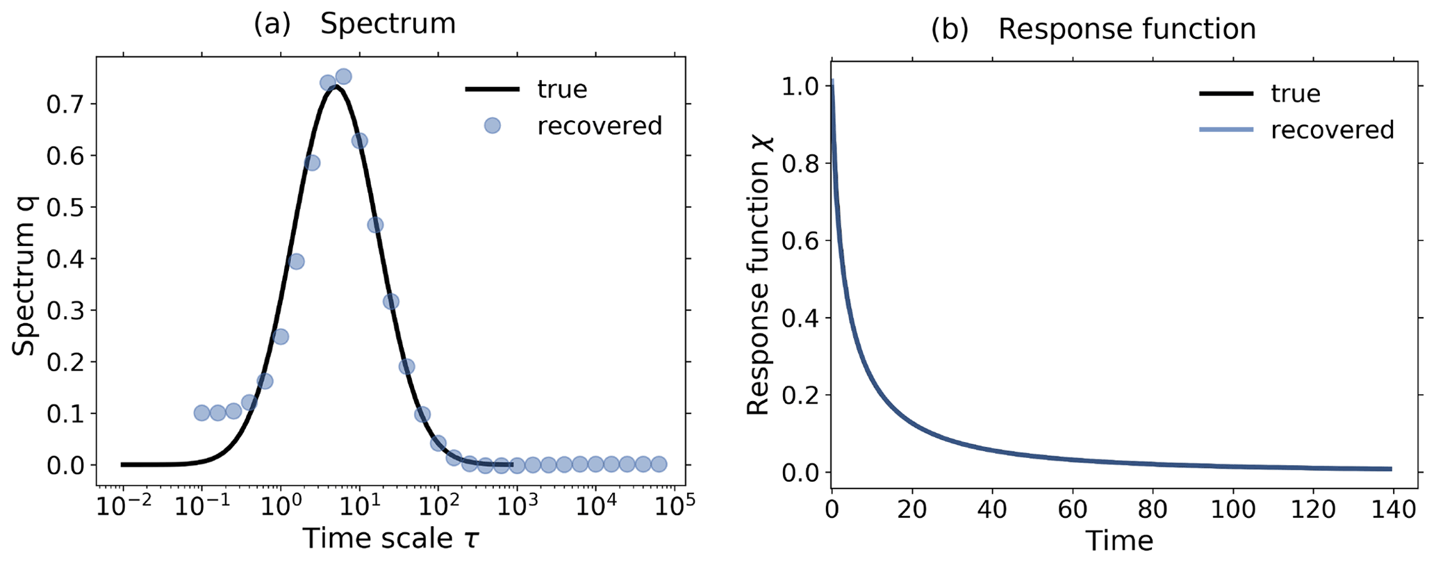
Figure E1Response function χ(t) and spectrum qλ recovered from toy model data taking the RFI parameters M=30, , and . Blue dots in (a) and blue line in (b) indicate the recovered values for the spectrum and for the response function, while black lines indicate their “true” values.

Figure E2Response function χ(t) and spectrum qλ recovered from toy model data taking the RFI parameters M=60, , and . Blue dots in (a) and blue line in (b) indicate the recovered values for the spectrum and for the response function, while black lines indicate their “true” values.
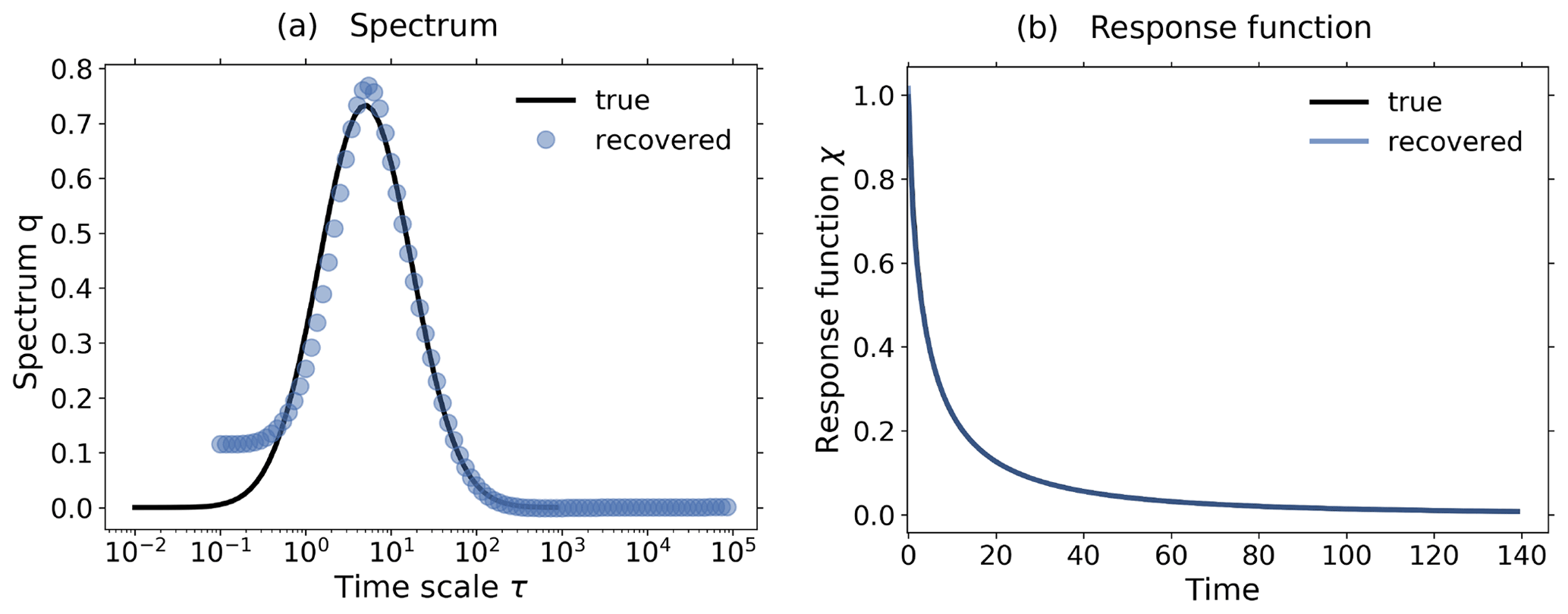
Figure E3Response function χ(t) and spectrum qλ recovered from toy model data taking the RFI parameters M=90, , and . Blue dots in (a) and blue line in (b) indicate the recovered values for the spectrum and for the response function, while black lines indicate their “true” values.
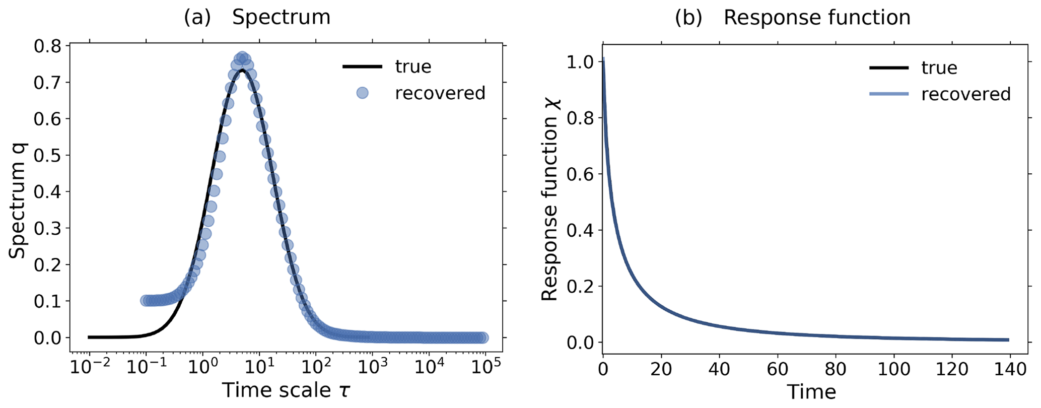
Figure E4Response function χ(t) and spectrum qλ recovered from toy model data taking the RFI parameters M=120, , and . Blue dots in (a) and blue line in (b) indicate the recovered values for the spectrum and for the response function, while black lines indicate their “true” values.

Figure E5Response function χ(t) and spectrum qλ recovered from toy model data taking the RFI parameters M=140, , and . Blue dots in (a) and blue line in (b) indicate the recovered values for the spectrum and for the response function, while black lines indicate their “true” values.
Figures E1–E5 show the recovery, taking the same limits used throughout the paper ( and ) but a different number of timescales M. Figures E6–E8 show the recovery, keeping the number of timescales and the lower limit used throughout the paper (M=30 and ) but changing the upper limit log τmax. Figures E9–E11 show the recovery, keeping the number of timescales and the upper limit used throughout the paper (M=30 and ) but changing the lower limit log τmax. As expected, the results are approximately independent of the changes in the prescribed parameters. The only substantial differences are found in the recovered spectra at timescales smaller than the time step Δt=1 and thus timescales over which anyway only little information is given by data. These small timescales are also problematic because of the ill-posedness of the problem that suppresses high-frequency information from the solution (see Groetsch, 1984, Sect. 1.1).
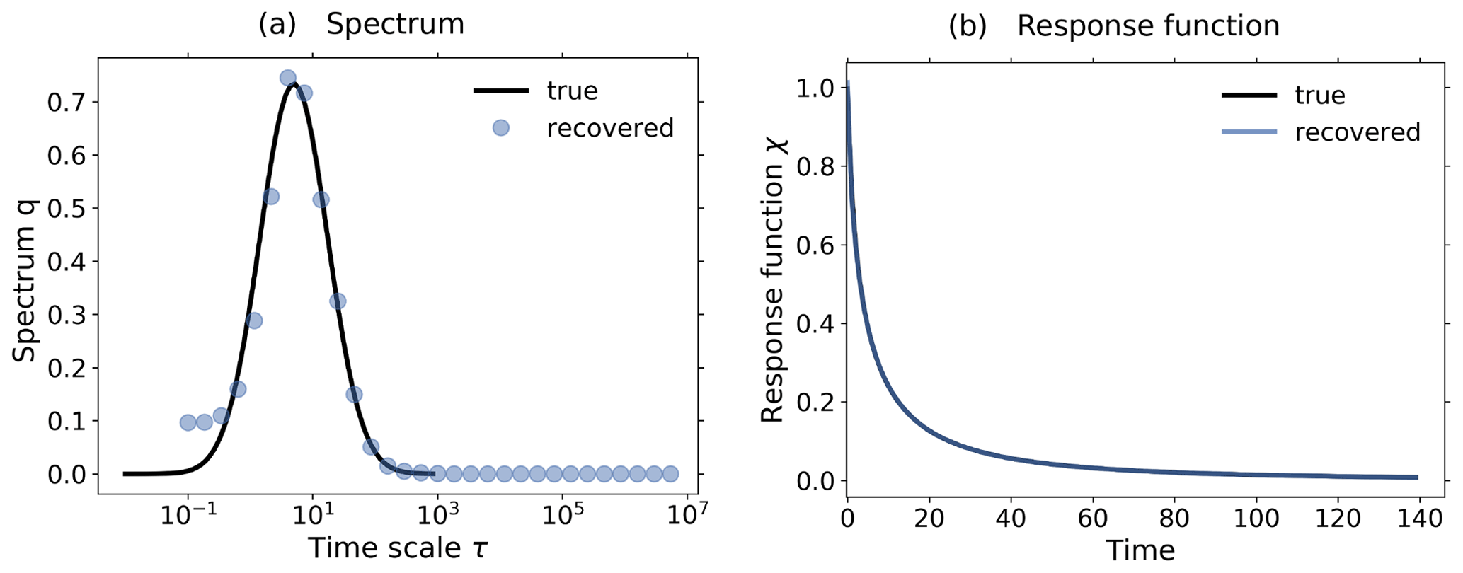
Figure E6Response function χ(t) and spectrum qλ recovered from toy model data taking the RFI parameters M=30, , and . Blue dots in (a) and blue line in (b) indicate the recovered values for the spectrum and for the response function, while black lines indicate their “true” values.
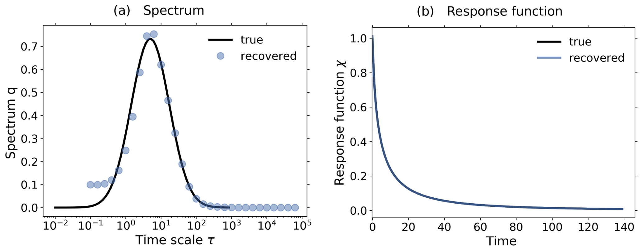
Figure E7Response function χ(t) and spectrum qλ recovered from toy model data taking the RFI parameters M=30, , and . Blue dots in (a) and blue line in (b) indicate the recovered values for the spectrum and for the response function, while black lines indicate their “true” values.
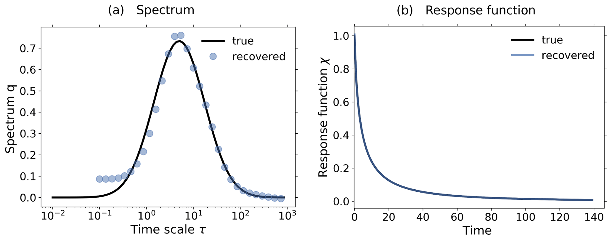
Figure E8Response function χ(t) and spectrum qλ recovered from toy model data taking the RFI parameters M=30, , and . Blue dots in (a) and blue line in (b) indicate the recovered values for the spectrum and for the response function, while black lines indicate their “true” values.

Figure E9Response function χ(t) and spectrum qλ recovered from toy model data taking the RFI parameters M=30, , and . Blue dots in (a) and blue line in (b) indicate the recovered values for the spectrum and for the response function, while black lines indicate their “true” values.
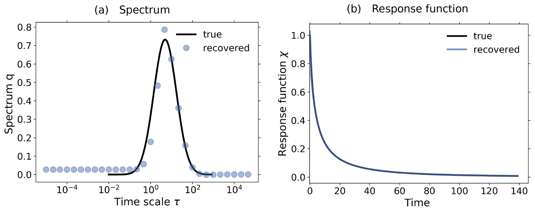
Figure E10Response function χ(t) and spectrum qλ recovered from toy model data taking the RFI parameters M=30, , and . Blue dots in (a) and blue line in (b) indicate the recovered values for the spectrum and for the response function, while black lines indicate their “true” values.
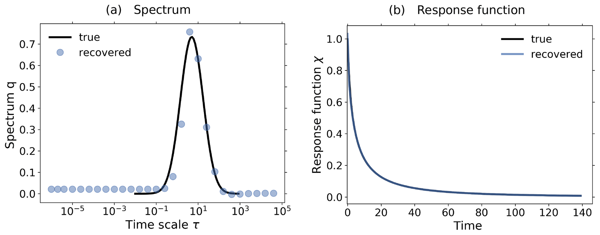
Figure E11Response function χ(t) and spectrum qλ recovered from toy model data taking the RFI parameters M=30, , and . Blue dots in (a) and blue line in (b) indicate the recovered values for the spectrum and for the response function, while black lines indicate their “true” values.
The scripts employed to produce the results in this paper as well as information on how to obtain the underlying data can be found at http://hdl.handle.net/21.11116/0000-0008-0F02-6 (last access: 2 October 2021, Torres Mendonca et al., 2021b).
The ideas for this study were jointly developed by all the authors. GLTM conducted the study and wrote the first draft. All the authors contributed to the final manuscript.
The authors declare that they have no conflict of interest.
Publisher's note: Copernicus Publications remains neutral with regard to jurisdictional claims in published maps and institutional affiliations.
We would like to thank Andreas Chlond, two anonymous referees, and Valerio Lucarini for very helpful suggestions on the manuscript.
The article processing charges for this open-access publication were covered by the Max Planck Society.
This paper was edited by Ilya Zaliapin and reviewed by three anonymous referees.
Abraham, R. and Marsden, J. E.: Foundations of Mechanics, 2nd edn., Benjamin, New York, NY, USA, 1982. a
Aengenheyster, M., Feng, Q. Y., van der Ploeg, F., and Dijkstra, H. A.: The point of no return for climate action: effects of climate uncertainty and risk tolerance, Earth Syst. Dynam., 9, 1085–1095, https://doi.org/10.5194/esd-9-1085-2018, 2018. a, b, c
Anderssen, R. S. and Bloomfield, P.: Numerical differentiation procedures for non-exact data, Numer. Math., 22, 157–182, 1974. a
Åström, K. J. and Eykhoff, P.: System identification – a survey, Automatica, 7, 123–162, 1971. a
Bakushinskii, A.: Remarks on choosing a regularization parameter using the quasi-optimality and ratio criterion, Comp. Math. Math. Phys.+, 24, 181–182, 1984. a
Baladi, V.: Dynamical zeta functions and dynamical determinants for hyperbolic maps, Springer, Switzerland, 2018. a
Beerends, R. J., ter Morsche, H. G., van den Berg, J. C., and van de Vrie, E. M.: Fourier and Laplace Transforms, Cambridge University Press, Cambridge, England, https://doi.org/10.1017/CBO9780511806834, 2003. a
Bertero, M.: Linear Inverse and Ill-Posed Problems, vol. 75 of Advances in Electronics and Electron Physics, Academic Press, New York, NY, USA, 1–120, https://doi.org/10.1016/S0065-2539(08)60946-4, 1989. a, b, c, d, e, f
Bertero, M., Boccacci, P., and Maggio, F.: Regularization methods in image restoration: an application to HST images, Int. J. Imag. Syst. Tech., 6, 376–386, 1995. a, b, c
Bódai, T., Lucarini, V., and Lunkeit, F.: Can we use linear response theory to assess geoengineering strategies?, Chaos, 30, 023124, https://doi.org/10.1063/1.5122255, 2020. a, b, c
Boulet, B. and Chartrand, L.: Fundamentals of signals and systems, Da Vinci Engineering Press, Hingham, MA, 2006. a
Caldeira, K. and Myhrvold, N.: Projections of the pace of warming following an abrupt increase in atmospheric carbon dioxide concentration, Environ. Res. Lett., 8, 034039, https://doi.org/10.1088/1748-9326/8/3/034039, 2013. a
Ciais, P., Sabine, C., Bala, G., Bopp, L., Brovkin, V., Canadell, J., Chhabra, A., DeFries, R., Galloway, J., Heimann, M., Jones, C., Le Quéré, C., Myneni, R., Piao, S., and Thornton, P.: Carbon and Other Biogeochemical Cycles, in: Climate Change 2013: The Physical Science Basis. Contribution of Working Group I to the Fifth Assessment Report of the Intergovernmental Panel on Climate Change, edited by: Stocker, T., Qin, D., Plattner, G.-K., Tignor, M., Allen, S., Boschung, J., Nauels, A., Xia, Y., Bex, V., and Midgley, P., Cambridge University Press, Cambridge, UK and New York, NY, USA, pp. 465–570, 2013. a
Colbourn, G., Ridgwell, A., and Lenton, T.: The time scale of the silicate weathering negative feedback on atmospheric CO2, Global Biogeochem. Cy., 29, 583–596, 2015. a, b
Emanuel, W. R., Killough, G. E., and Olson, J. S.: Modelling the Circulation of Carbon in the World's Terrestrial Ecosystems, SCOPE, 16, 335–353, 1981. a
Engl, H. W., Hanke, M., and Neubauer, A.: Regularization of inverse problems, vol. 375, Springer Science & Business Media, Dordrecht, The Netherlands, 1996. a, b, c, d, e, f, g, h
Enting, I. : Ambiguities in the calibration of carbon cycle models, Inverse Problems, 6, L39, https://doi.org/10.1088/0266-5611/6/5/001, 1990. a
Enting, I. and Clisby, N.: Estimates of climatic influence on the carbon cycle, Earth Syst. Dynam. Discuss. [preprint], https://doi.org/10.5194/esd-2019-41, 2019. a
Enting, I. and Mansbridge, J.: Inversion relations for the deconvolution of CO2 data from ice cores, Inverse Problems, 3, L63–L69, 1987. a
Eyring, V., Bony, S., Meehl, G. A., Senior, C. A., Stevens, B., Stouffer, R. J., and Taylor, K. E.: Overview of the Coupled Model Intercomparison Project Phase 6 (CMIP6) experimental design and organization, Geosci. Model Dev., 9, 1937–1958, https://doi.org/10.5194/gmd-9-1937-2016, 2016. a
Forney, D. C. and Rothman, D. H.: Inverse method for estimating respiration rates from decay time series, Biogeosciences, 9, 3601–3612, https://doi.org/10.5194/bg-9-3601-2012, 2012. a, b, c
Gallavotti, G.: Nonequilibrium and irreversibility, Springer, Berlin/Heidelberg, Germany, 2014. a
Gasser, T., Peters, G. P., Fuglestvedt, J. S., Collins, W. J., Shindell, D. T., and Ciais, P.: Accounting for the climate–carbon feedback in emission metrics, Earth Syst. Dynam., 8, 235–253, https://doi.org/10.5194/esd-8-235-2017, 2017. a
Ghil, M. and Lucarini, V.: The physics of climate variability and climate change, Rev. Mod. Phys., 92, 035002, https://doi.org/10.1103/RevModPhys.92.035002, 2020. a, b
Golub, G. H. and Van Loan, C. F.: Matrix Computations, The Johns Hopkins University Press, Baltimore, Maryland, 1996. a, b
Gottwald, G.: Introduction to Focus Issue: Linear response theory: Potentials and limits, Chaos, 30, 020401, https://doi.org/10.1063/5.0003135, 2020. a
Gottwald, G. A., Wormell, J., and Wouters, J.: On spurious detection of linear response and misuse of the fluctuation–dissipation theorem in finite time series, Physica D, 331, 89–101, 2016. a
Grieser, J. and Schönwiese, C.-D.: Process, Forcing, and Signal Analysis of Global Mean Temperature Variations by Means of a Three-Box Energy Balance Model, Climatic Change, 48, 617–646, 2001. a
Groetsch, C.: Comments on Morozov's discrepancy principle, in: Improperly posed problems and their numerical treatment, edited by: Hämmerlin, G. and Hoffmann, K. H., Springer, Berlin/Heidelberg, Germany, pp. 97–104, 1983. a
Groetsch, C.: The theory of Tikhonov regularization for Fredholm equations, Boston Pitman Publication, Boston, MA, 1984. a, b, c, d, e, f, g, h, i, j, k, l, m, n
Groetsch, C. W.: Integral equations of the first kind, inverse problems and regularization: a crash course, J. Phys. Conf. Ser., 73, 012001, https://doi.org/10.1088/1742-6596/73/1/012001, 2007. a, b
Großmann, S.: Linear response in chaotic states of discrete dynamics, Z. Phys. B Con. Mat., 57, 77–84, 1984. a
Hairer, M. and Majda, A. J.: A simple framework to justify linear response theory, Nonlinearity, 23, 909, https://doi.org/10.1088/0951-7715/23/4/008, 2010. a
Hämarik, U., Palm, R., and Raus, T.: Comparison of parameter choices in regularization algorithms in case of different information about noise level, Calcolo, 48, 47–59, 2011. a
Hänggi, P. and Thomas, H.: Stochastic processes: Time evolution, symmetries and linear response, Phys. Rep., 88, 207–319, 1982. a
Hansen, P. C.: The truncated SVD as a method for regularization, BIT, 27, 534–553, 1987. a
Hansen, P. C.: Regularization, GSVD and truncated GSVD, BIT, 29, 491–504, 1989. a
Hansen, P. C.: The discrete Picard condition for discrete ill-posed problems, BIT, 30, 658–672, 1990. a, b, c
Hansen, P. C.: Numerical tools for analysis and solution of Fredholm integral equations of the first kind, Inverse Problems, 8, 849, https://doi.org/10.1088/0266-5611/8/6/005, 1992. a, b, c
Hansen, P. C.: Deconvolution and regularization with Toeplitz matrices, Num. Algorithms, 29, 323–378, 2002. a
Hansen, P. C.: Discrete inverse problems: insight and algorithms, SIAM, 7, https://doi.org/10.1137/1.9780898718836, 2010. a, b, c, d
Hasselmann, K., Sausen, R., Maier-Reimer, E., and Voss, R.: On the cold start problem in transient simulations with coupled atmosphere-ocean models, Clim. Dynam., 9, 53–61, 1993. a, b, c, d
Hasselmann, K., Hasselmann, S., Giering, R., Ocana, V., and Storch, H.: Sensitivity study of optimal CO2 emission paths using a simplified structural integrated assessment model (SIAM), Climatic Change, 37, 345–386, 1997. a
Isermann, R. and Münchhof, M.: Identification of dynamic systems: an introduction with applications, Springer Science & Business Media, Berlin, Germany, 2010. a
Istratov, A. A. and Vyvenko, O. F.: Exponential analysis in physical phenomena, Rev. Sci. Instrum., 70, 1233–1257, 1999. a, b, c, d
Joos, F. and Bruno, M.: Pulse response functions are cost-efficient tools to model the link between carbon emissions, atmospheric CO2 and global warming, Phys. Chem. Earth, 21, 471–476, 1996. a, b
Joos, F., Bruno, M., Fink, R., Siegenthaler, U., Stocker, T. F., Le Quere, C., and Sarmiento, J. L.: An efficient and accurate representation of complex oceanic and biospheric models of anthropogenic carbon uptake, Tellus B, 48, 397–417, 1996. a, b, c
Joos, F., Roth, R., Fuglestvedt, J. S., Peters, G. P., Enting, I. G., von Bloh, W., Brovkin, V., Burke, E. J., Eby, M., Edwards, N. R., Friedrich, T., Frölicher, T. L., Halloran, P. R., Holden, P. B., Jones, C., Kleinen, T., Mackenzie, F. T., Matsumoto, K., Meinshausen, M., Plattner, G.-K., Reisinger, A., Segschneider, J., Shaffer, G., Steinacher, M., Strassmann, K., Tanaka, K., Timmermann, A., and Weaver, A. J.: Carbon dioxide and climate impulse response functions for the computation of greenhouse gas metrics: a multi-model analysis, Atmos. Chem. Phys., 13, 2793–2825, https://doi.org/10.5194/acp-13-2793-2013, 2013. a, b, c, d, e
Kubo, R.: Statistical-mechanical theory of irreversible processes. I. General theory and simple applications to magnetic and conduction problems, J. Phys. Soc. Jpn., 12, 570–586, 1957. a
Kumaresan, R., Tufts, D., and Scharf, L. L.: A Prony method for noisy data: Choosing the signal components and selecting the order in exponential signal models, P. IEEE, 72, 230–233, 1984. a
Kuo, F.: Network Analysis and Synthesis, Wiley, New York, NY, USA and London, England, 1966. a
Lamm, P. K.: Approximation of ill-posed Volterra problems via predictor–corrector regularization methods, SIAM J. Appl. Math., 56, 524–541, 1996. a
Lanczos, C.: Applied Analysis, Mathematics series, Prentice-Hall, Englewood Cliffs, NJ, 1956. a, b
Landl, G., Langthaler, T., Englt, H. W., and Kauffmann, H. F.: Distribution of event times in time-resolved fluorescence: the exponential series approach–algorithm, regularization, analysis, J. Comput. Phys., 95, 1–28, 1991. a
Lembo, V., Lucarini, V., and Ragone, F.: Beyond forcing scenarios: predicting climate change through response operators in a coupled general circulation model, Sci. Rep.-UK, 10, 1–13, 2020. a
Levin, E. and Meltzer, A. Y.: Estimation of the regularization parameter in linear discrete ill-posed problems using the Picard parameter, SIAM J. Sci. Comput., 39, A2741–A2762, 2017. a
Li, S. and Jarvis, A.: Long run surface temperature dynamics of an A-OGCM: the HadCM3 4× CO2 forcing experiment revisited, Clim. Dynam., 33, 817–825, 2009. a
Lord, N. S., Ridgwell, A., Thorne, M., and Lunt, D.: An impulse response function for the “long tail” of excess atmospheric CO2 in an Earth system model, Global Biogeochem. Cy., 30, 2–17, 2016. a, b
Lucarini, V.: Response theory for equilibrium and non-equilibrium statistical mechanics: Causality and generalized Kramers-Kronig relations, J. Stat. Phys., 131, 543–558, 2008. a
Lucarini, V.: Evidence of dispersion relations for the nonlinear response of the Lorenz 63 system, J. Stat. Phys., 134, 381–400, 2009. a, b, c
Lucarini, V. and Sarno, S.: A statistical mechanical approach for the computation of the climatic response to general forcings, Nonlin. Processes Geophys., 18, 7–28, https://doi.org/10.5194/npg-18-7-2011, 2011. a, b
Lucarini, V., Blender, R., Herbert, C., Ragone, F., Pascale, S., and Wouters, J.: Mathematical and physical ideas for climate science, Rev. Geophys., 52, 809–859, https://doi.org/10.1002/2013RG000446, 2014. a, b
Lucarini, V., Ragone, F., and Lunkeit, F.: Predicting climate change using response theory: Global averages and spatial patterns, J. Stat. Phys., 166, 1036–1064, 2017. a, b, c, d, e, f
MacMartin, D. G. and Kravitz, B.: Dynamic climate emulators for solar geoengineering, Atmos. Chem. Phys., 16, 15789–15799, https://doi.org/10.5194/acp-16-15789-2016, 2016. a, b, c, d
Maier-Reimer, E. and Hasselmann, K.: Transport and storage of CO2 in the ocean – an inorganic ocean-circulation carbon cycle model, Clim. Dynam., 2, 63–90, 1987. a, b, c, d, e, f
Morozov, V. A.: On the solution of functional equations by the method of regularization, Dokl. Akad. Nauk.+, 167, 510–512, 1966. a
Ni, A.: Approximating linear response by non-intrusive shadowing algorithms, arXiv [preprint], arXiv:2003.09801, 25 December 2020. a
Ni, A. and Wang, Q.: Sensitivity analysis on chaotic dynamical systems by Non-Intrusive Least Squares Shadowing (NILSS), J. Comput. Phys., 347, 56–77, 2017. a
Olshevsky, D. E.: Integral Equations as a Method of Theoretical Physics, Am. Math. Mon., 37, 274–281, https://doi.org/10.1080/00029890.1930.11987073, 1930. a
Palm, R.: Numerical comparison of regularization algorithms for solving ill-posed problems, PhD thesis, Tartu University Press, Tartu, Estonia, 2010. a
Phillips, D. L.: A technique for the numerical solution of certain integral equations of the first kind, J. ACM, 9, 84–97, 1962. a
Pillonetto, G., Dinuzzo, F., Chen, T., De Nicolao, G., and Ljung, L.: Kernel methods in system identification, machine learning and function estimation: A survey, Automatica, 50, 657–682, 2014. a
Polyanin, A. and Manzhirov, A.: Handbook of Integral Equations, Taylor & Francis, New York, NY, USA, 1998. a
Pongratz, J., Caldeira, K., Reick, C. H., and Claussen, M.: Coupled climate–carbon simulations indicate minor global effects of wars and epidemics on atmospheric CO2 between ad 800 and 1850, Holocene, 21, 843–851, 2011. a, b, c
Ragone, F., Lucarini, V., and Lunkeit, F.: A new framework for climate sensitivity and prediction: a modelling perspective, Clim. Dynam., 46, 1459–1471, 2016. a, b, c, d, e, f, g
Reick, C. H.: Linear response functions of chaotic systems and equilibrium moments, Math. Comput. Simulat., 40, 281–295, 1996. a
Reick, C. H.: Linear response of the Lorenz system, Phys. Rev. E, 66, 036103, https://doi.org/10.1103/PhysRevE.66.036103, 2002. a, b
Ricke, K. L. and Caldeira, K.: Maximum warming occurs about one decade after a carbon dioxide emission, Environ. Res. Lett., 9, 124002, https://doi.org/10.1088/1748-9326/9/12/124002, 2014. a
Risken, H.: The Fokker-Planck Equation, 2nd edn., Springer, Berlin, 1996. a
Ruelle, D.: Differentiation of SRB states, Commun. Math. Phys., 187, 227–241, 1997. a
Ruelle, D.: General linear response formula in statistical mechanics, and the fluctuation-dissipation theorem far from equilibrium, Phys. Lett. A, 245, 220–224, 1998. a
Ruelle, D.: Smooth dynamics and new theoretical ideas in nonequilibrium statistical mechanics, J. Stat. Phys., 95, 393–468, 1999. a
Ruelle, D.: A review of linear response theory for general differentiable dynamical systems, Nonlinearity, 22, 855, https://doi.org/10.1088/0951-7715/22/4/009, 2009. a
Rugh, W.: Nonlinear System Theory: The Volterra/Wiener Approach, Johns Hopkins series in information sciences and systems, Johns Hopkins University Press, Baltimore, Maryland, 1981. a
Schetzen, M.: Nonlinear System Modelling and Analysis from the Volterra and Wiener Perspective, Springer London, London, 13–24, https://doi.org/10.1007/978-1-84996-513-2_2, 2010. a
Siegenthaler, U. and Oeschger, H.: Predicting future atmospheric carbon dioxide levels, Science, 199, 388–395, 1978. a, b, c
Śliwiak, A. A., Chandramoorthy, N., and Wang, Q.: Computational assessment of smooth and rough parameter dependence of statistics in chaotic dynamical systems, Commun. Nonlinear Sci., 101, 105906, 2021. a
Söderström, T. and Stoica, P.: System identification, Prentice-Hall International, Upper Saddle River, NJ, 1989. a
Taroudaki, V. and O'Leary, D. P.: Near-optimal spectral filtering and error estimation for solving ill-posed problems, SIAM J. Sci. Comput., 37, A2947–A2968, 2015. a
Taylor, K. E., Stouffer, R. J., and Meehl, G. A.: An overview of CMIP5 and the experiment design, B. Am. Meteorol. Soc., 93, 485–498, 2012. a
Thompson, M. V. and Randerson, J. T.: Impulse response functions of terrestrial carbon cycle models: method and application, Glob. Change Biol., 5, 371–394, 1999. a, b, c
Tikhonov, A. N.: Solution of incorrectly formulated problems and the regularization method, Dokl. Akad. Nauk.+, 151, 1035–1038, 1963. a
Torres Mendonça, G. L., Pongratz, J., and Reick, C. H.: Identification of linear response functions from arbitrary perturbation experiments in the presence of noise – Part 2: Application to the land carbon cycle in the MPI Earth System Model, Nonlin. Processes Geophys., 28, 533–564, https://doi.org/10.5194/npg-28-533-2021, 2021a. a
Torres Mendonca, G., Pongratz, J., and Reick, C. H.: Supplementary material for “Identification of linear response functions from arbitrary perturbation experiments in the presence of noise – Part I. Method development and toy model demonstration”, MPG Publication Repository – MPG.PuRe [code], available at: http://hdl.handle.net/21.11116/0000-0008-0F02-6, last access: 2 October 2021b. a
van Zalinge, B. C., Feng, Q. Y., Aengenheyster, M., and Dijkstra, H. A.: On determining the point of no return in climate change, Earth Syst. Dynam., 8, 707–717, https://doi.org/10.5194/esd-8-707-2017, 2017. a, b
Volterra, V.: Theory of Functionals and of Integral and Integro-differential Equations, Dover Books on Intermediate and Advanced Mathematics, Dover Publications, New York, NY, USA, 1959. a
Wormell, C. L. and Gottwald, G. A.: On the validity of linear response theory in high-dimensional deterministic dynamical systems, J. Stat. Phys., 172, 1479–1498, 2018. a
Wormell, C. L. and Gottwald, G. A.: Linear response for macroscopic observables in high-dimensional systems, Chaos, 29, 113127, https://doi.org/10.1063/1.5122740, 2019. a
- Abstract
- Introduction
- Linear response theory and basic ansatz of the method
- Identification of linear response functions from arbitrary perturbation experiments
- Applicability in the presence of noise and nonlinearities
- Comparison with previous methods
- Summary, discussion, and outlook
- Appendix A: Basic equations in this study are Fredholm equations of the first kind
- Appendix B: Derivation of Eqs. (11) and (12) on which our study is based
- Appendix C: Spectrum q(τ) positive or negative for all τ implies χ(t) is monotonic
- Appendix D: Response function and noise in the nonlinearized response for the toy model
- Appendix E: Sensitivity of the recovered response function and spectrum to the parameters M, log τmin, and log τmax of the RFI algorithm
- Code and data availability
- Author contributions
- Competing interests
- Disclaimer
- Acknowledgements
- Financial support
- Review statement
- References