the Creative Commons Attribution 4.0 License.
the Creative Commons Attribution 4.0 License.
 | 20 Apr 2021
Extracting statistically significant eddy signals from large Lagrangian datasets using wavelet ridge analysis, with application to the Gulf of Mexico
Jonathan M. Lilly
Paula Pérez-Brunius
A method for objectively extracting the displacement signals associated with coherent eddies from Lagrangian trajectories is presented, refined, and applied to a large dataset of 3770 surface drifters from the Gulf of Mexico. The method, wavelet ridge analysis, is a general method for the analysis of modulated oscillations, here modified to be more suitable to the eddy-detection problem. A means for formally assessing statistical significance is introduced, addressing the issue of false positives arising by chance from an unstructured turbulent background and opening the door to confident application of the method to very large datasets. Significance is measured through a frequency-dependent comparison with a stochastic dataset having statistical and spectral properties that match the original, but lacking organized oscillations due to eddies or waves. The application to the Gulf of Mexico reveals major asymmetries between cyclones and anticyclones, with anticyclones dominating at radii larger than about 50 km, but an unexpectedly rich population of highly nonlinear cyclones dominating at smaller radii. Both the method and the Gulf of Mexico eddy dataset are made freely available to the community for noncommercial use in future research.
- Article
(13973 KB) - Full-text XML
- Companion paper
- BibTeX
- EndNote


Trajectories from freely drifting, or Lagrangian, instruments are one of the major windows into observing the ocean circulation. A perennial theme in oceanography is the study of long-lived vortex structures, also known as coherent eddies, and their role in influencing the large-scale circulation. On account of these two factors, an important data analysis problem is to be able to accurately, objectively,1 and automatically detect signals in Lagrangian data arising from instruments trapped in eddies and to use these extracted signals to estimate the physical properties of the eddies themselves.
Obtaining a satisfactory solution to this problem that could scale to very large datasets would enable a rigorous eddy census of the entire surface drifter dataset from NOAA's Global Drifter Program (Lumpkin and Pazos, 2007), currently consisting of about 25 000 trajectories. It would also, significantly, permit one to compare an eddy census from real-world surface drifters with those from synthetic trajectories in high-resolution numerical models. This type of Lagrangian model–data intercomparison offers considerable potential for refining models and also for querying the models to better understand what is being observed in data, but this is not yet possible due to limitations of available analysis methods.
The problem of identifying and estimating the properties of coherent eddies in Lagrangian trajectories should be distinguished from the problem of describing the aggregate forms of trajectories due to the eddies they contain. To help clarify this, we introduce the term “eddy signal” to mean the displacement of a particle about an eddy's center. We would then see a trajectory as a superposition of different types of signals: e.g., an eddy signal, a near-inertial signal, and a mean flow. Whereas methods such as that of Dong et al. (2011) as well as the spin parameter method of Veneziani et al. (2005a, b) are concerned with identifying or modeling the aggregate trajectory, here we are interested in identifying and extracting eddy signals themselves. This interest complements examinations of the statistical imprint of eddies on trajectories using the spin parameter approach (Griffa et al., 2008; Lumpkin, 2016; Cetina-Heredia et al., 2019).
Identifying eddies in trajectories is sometimes equated with finding trajectories that execute loops, and indeed the term “looper” is sometimes used to mean “a trajectory containing an eddy”. However, one must be very cautious about forming this equivalence as there is not a one-to-one relationship between trajectory loops and particle displacements due to eddy currents. Simply changing the value of an advecting flow will alter the appearance of, or even eliminate, trajectory loops for a given eddy signal. Similarly, a trajectory can form a loop for many reasons that do not involve a coherent eddy. For these reasons, eddy detections and property estimates based solely on the visual appearance of trajectories should be considered only as rough approximations.
Various methods have been proposed over the years for identifying and extracting eddy signals from Lagrangian trajectories (e.g., Kirwan et al., 1984, 1988; Armi et al., 1989; Flament et al., 2001; Testor and Gascard, 2003; Lankhorst, 2006); see Dong et al. (2011) for a useful review. Generally speaking, a difficulty faced by such methods is that fact that the frequency of the eddy signal is not only unknown a priori, but it also tends to vary substantially with time, as seen for example in Flament et al. (2001). This frequency modulation makes the study of eddy signals substantially more difficult than, for example, studying tides, which occur at known and fixed frequencies. Narrowband methods such as bandpassing or complex demodulation would therefore perform quite poorly. In order to accommodate such frequency modulation, the above methods generally contain free parameters that must be chosen by an analyst. Because of the need for hand tuning for individual trajectories, applications of such methods to large datasets would be problematic.
A major step in the eddy extraction problem was taken by Lilly and Gascard (2006). In that paper, an innovative and powerful method from signal analysis termed wavelet ridge analysis (Delprat et al., 1992; Mallat, 1999) was modified for application to Lagrangian trajectories. That method is designed to detect and analyze modulated oscillations, that is, oscillations whose amplitude and frequency vary as a function of time. This type of signal accords well with our physical expectations for the displacement of a particle trapped in a vortex. The wavelet ridge method is able to automatically extract frequency-modulated signals occurring somewhere within a chosen range of frequencies, without the need to tune parameters for an individual time series. A compelling aspect of this method is that it begins with the specification of the type of object we are looking for, namely, a modulated oscillation, a type of signal for which there exists a solid theoretical foundation (Gabor, 1946; Picinbono, 1997).
An application of the wavelet ridge analysis method to trajectories from a numerical model of an unstable jet on a beta plane (Lilly et al., 2011) showed that the method could accurately and automatically extract eddy signals from a set of 100 trajectories and that these could be unambiguously discriminated from oscillatory signals due to Rossby waves or jet meander. The wavelet ridge analysis method has been employed by a number of other authors (e.g., Garreau et al., 2011; Alpers et al., 2013; Bower et al., 2013; Le Hénaff et al., 2014; Inoue et al., 2016; Kourafalou et al., 2017; Furey et al., 2018; de Jong et al., 2018; Le Hénaff et al., 2020) using the software implementation created by Lilly and Gascard (2006) and appears to now be the standard method for extracting eddy signals from Lagrangian data. The method was further refined and extended in a series of follow-up papers (Lilly and Olhede, 2009a, 2010b, 2012a), including the treatment of bias errors arising from modulation strength in Lilly and Olhede (2010a, 2012a).
The wavelet ridge analysis method allows one to readily analyze datasets with dozens or perhaps hundreds of trajectories. However, there is a major challenge which prevents it – or any other eddy-extraction method – from being immediately applicable to very large datasets consisting of thousands or tens of thousands of trajectories. This is the problem of false-positive features arising from the interaction of the detection method with the turbulent background flow. For small to medium-size datasets such events may be readily identified with a visual scan, but that subjective operation becomes unwieldy for larger datasets.
In previous work (Lilly et al., 2017), we have shown that Lagrangian trajectories in forced-dissipative quasigeostrophic turbulence can be usefully separated into two classes: those that contain high-frequency oscillatory signals associated with trapping within coherent eddies and those that do not. Trajectories in the latter class are remarkably similar to those resulting from a type of damped random walk; see Figs. 2 and 3 therein. This supports the conceptual model that trajectories containing eddies consist of the sum of an eddy signal, superposed on a stochastic process that arises from geostrophic turbulence and that may be considered “noise” from the point of view of detecting eddies.
The stochastic background flow can be the source of spurious features that masquerade as coherent eddies, a phenomenon that can be understood as follows. In the one-dimensional case, a discrete random walk is intuitively described as a drunk staggering between lampposts. In the two-dimensional case, the drunk has a grid of lampposts available for their staggering. From time to time the drunk will, by chance, happen to turn in a circle or oscillate back and forth between two lampposts. This illustrates why, in applying the wavelet ridge analysis to time series of stochastic processes analogous to the random walk, oscillatory events are occasionally detected. One would not wish to confuse random features arising from the turbulent background with the organized oscillations due to coherent eddies.
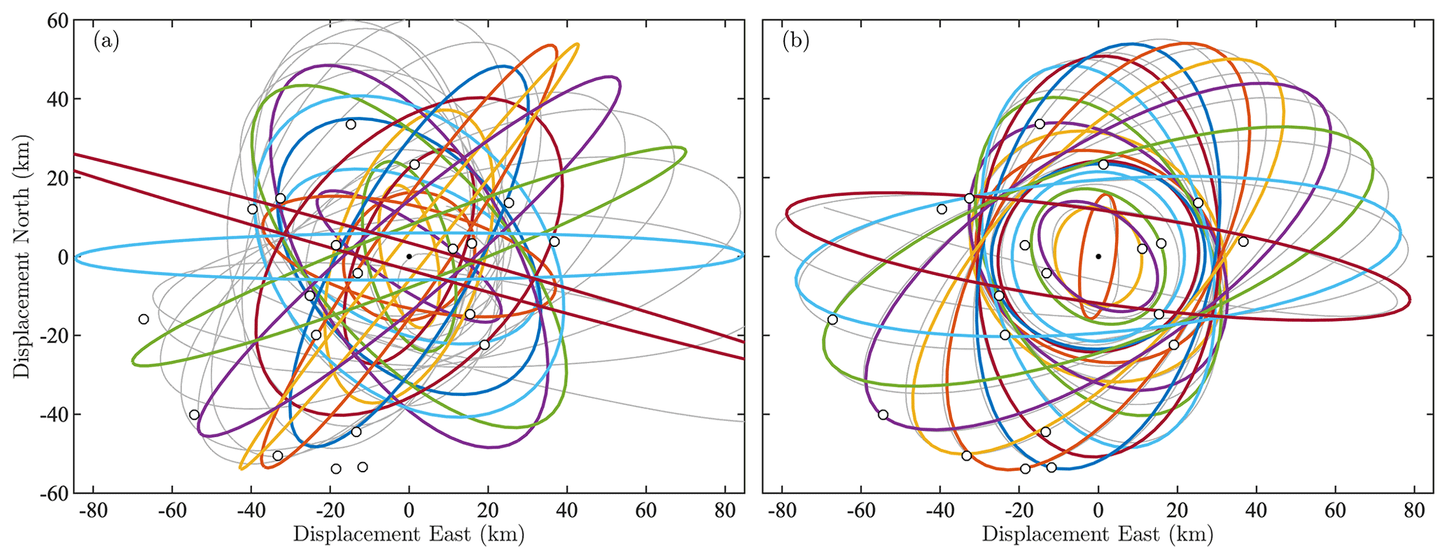
This paper has three objectives. Firstly, the ridge analysis method of Lilly and Gascard (2006) is streamlined and updated with several important refinements, a deeper discussion of the connection to signal processing theory, and with sufficient background on the wavelet transform itself so as to be self-contained. Secondly, the method is applied to a set of several thousand drifter trajectories from the Gulf of Mexico (see Fig. 1), leading to the identification of a set of statistically significant eddy signals, shown in Fig. 2. This Gulf of Mexico eddy dataset is freely distributed to the community for noncommercial uses, as described at the end of the paper, and is being used in a sequel to investigate the eddy dynamics in this environmentally and societally important region. Finally, the false-positive problem is solved through the application of the ridge analysis method to a synthetically created noise dataset matching the basic statistical properties of the observations, together with the introduction of an innovative frequency-dependent significance criterion.
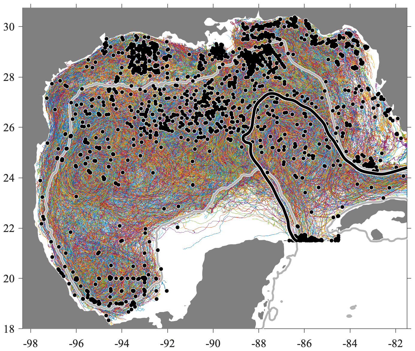
Figure 1Surface drifter trajectories in the Gulf of Mexico from the consolidated dataset of Lilly and Pérez-Brunius (2021a). Colors correspond to different trajectories, the beginning of each of which is marked by a black dot. In this and the following plot, the heavy gray contour is the 500 m isobath, while the heavy black line outlines the estimated location of the time-mean Loop Current. Specifically, the black contour marks the location at which the drifter-estimated time-mean speed from Fig. 3a of Lilly and Pérez-Brunius (2021a) is equal to 70 cm s−1. The southern edge of the study region in this figure and in Fig. 2 is delineated by a dotted line extending east from the Yucatán Peninsula along 21.5∘ N, then turning north to Cuba at 84.5∘ W; it is mostly obscured by the black dots marking trajectories entering the region.
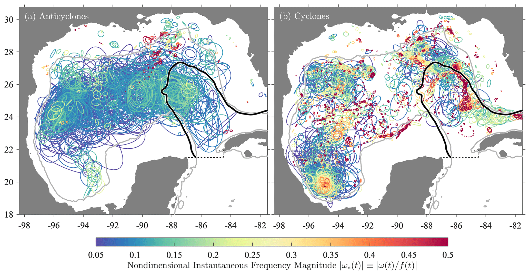
Figure 2Ellipses from all statistically significant eddy signals in the dataset shown in Fig. 1 detected using the method described here, with anticyclonic events in (a) and cyclonic events in (b). The time interval between successive ellipses is equal to the estimated period of the oscillation, , where ω(t) is the instantaneous frequency defined subsequently in Eq. (34). The colored shading is the nondimensional instantaneous frequency magnitude , in which ω(t) has been normalized by the Coriolis frequency at the latitude of the ellipse's center, denoted f⋄(t). It will be shown that is an estimate of the local Rossby number of the oscillatory flow. Ellipses are plotted in reverse order of their value, thus placing higher-frequency, more nonlinear features on top. The asymmetry between cyclonic and anticyclonic features is strikingly apparent. Other lines are as in Fig. 1.
As motivation for the investment required in learning this method, the results of the application to the Gulf of Mexico will be briefly described at the outset. The dataset to be analyzed in this work is a set of 3770 surface drifter trajectories, compiled from a variety of experiments, processed, and quality controlled as described in Lilly and Pérez-Brunius (2021a), shown in Fig. 1. Applying the method developed here, one is able to extract from the drifter trajectories a set of contiguous, possibly overlapping displacement signals consisting of modulated oscillations in two dimensions. The portion of such signals judged to be statistically significant, in the sense of occurring at a rate at least 10× greater than that expected under the noise hypothesis, is identified. These are visualized in Fig. 2 as a series of ellipses, colored here by a nondimensional frequency magnitude that when multiplied by 2 becomes a measure of Rossby number.
The distributions of cyclonic and anticyclonic events are completely different. The dense populations of large anticyclonic eddies filling the central Gulf of Mexico are the well-known Loop Current Eddies (e.g., Elliott, 1982; Lipphardt et al., 2008; Hall and Leben, 2016). These shed periodically from the energetic Loop Current, then propagate westward. Only a handful of small, intense anticyclones are observed, mostly located between the Loop Current and the Mississippi outflow region. On the cyclonic side, a hotspot of activity is seen in the southern Gulf of Mexico, corresponding to a persistent cyclonic eddy known as the Campeche Gyre (Padilla-Pilotze, 1990; Vázquez De La Cerda et al., 2005; Pérez-Brunius et al., 2013). On the periphery of the Loop Current, intense mesoscale cyclones are seen, the Loop Current Frontal Eddies (LCFEs); see, e.g., Le Hénaff et al. (2014). Similar features occur also in the western Gulf of Mexico but are of an unknown origin. In what appears to be a new result, sub-10 km, submesocale eddies with Rossby numbers approaching or exceeding unity are found throughout the region, visible in this plot as small red circles. This figure is an unprecedented view of the eddy activity in the Gulf of Mexico and illustrates the potential of the method to illuminate aspects of the circulation that are otherwise buried in trajectories.
The structure of the paper is as follows. A mathematical model for the motion of a particle trapped in an eddy is presented in Sect. 2. The means of extracting such signals from displacement time series that are also influenced by a turbulent background flow is developed in Sect. 3, building on Lilly and Gascard (2006) and subsequent work. The application to the Gulf of Mexico and the creation of a statistical significance measure are accomplished in Sect. 4. A brief discussion of the statistically significant eddy events is then given, followed by the Conclusions. Further examination of the Gulf of Mexico eddy signals and their implications for eddy dynamics and life cycles in this region is left to a sequel. All code developed for this paper is distributed as a part of a freely available MATLAB toolbox, including a convenient and self-contained eddy extraction function, as described following the Conclusions. Finally the Gulf of Mexico Eddy Dataset (GOMED), which includes the signals shown in Fig. 2 and their ellipse parameters, is described. Because a large number of different mathematical symbols are used in this paper, Table A1, located after the Conclusions, presents an overview of some of the most important ones.
This section describes a mathematical method for the displacement signal of a particle trapped in coherent eddy, building on the formulations in Lilly and Gascard (2006), Lilly et al. (2011), and Lilly and Olhede (2012a).
2.1 The modulated elliptical signal
The displacement signal of an instrument or particle advected by an eddy, within a moving frame of reference centered on the eddy's center – what we refer to as an “eddy signal” for short – will be modeled as the trajectory traced out by a particle orbiting a time-varying ellipse. We will use the complex-valued notation , with , and with x(t) and y(t) being the east–west and north–south displacements from the eddy center, respectively. Such a signal can be written as
where a(t) and b(t) are the semi-major and semi-minor axes, θ(t) is the orientation angle of the major axis with respect to the x axis, and ϕ(t) is a phase setting the position of the particle along the ellipse periphery. While is always positive, b(t) can be of either sign and encodes the direction in which the ellipse is being orbited, with positive b(t) corresponding to counterclockwise motion. Equation (1) will be called the ellipse generation equation.
A schematic of an ellipse is presented in Fig. 3. The geometric angle between the major axis and the particle position, denoted φ(t) in this plot, is related to the phase ϕ(t) that appears in Eq. (1) by2
such that φ(t) can be recovered from the phase ϕ(t) via
where ℑ{⋅} denotes the imaginary part. The combination ℑ{log [⋅]} is used here to implement the four-quadrant inverse tangent function, since ℑ{log eiϑ}=ϑ.
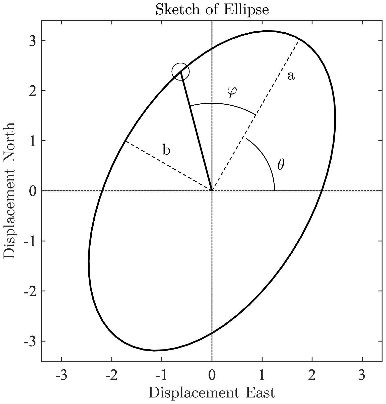
Figure 3A schematic of a particle orbiting an ellipse, as described by Eq. (1). The semi-major axis a(t), semi-minor axis b(t), orientation angle θ(t), and particle position angle φ(t) are all labeled. The circle denotes the instantaneous particle position. Here a(t)=3.5, b(t)=2, and . These values imply together with and , with the latter two quantities defined subsequently in Sect. 2.2.
The type of signal described by Eq. (1) is referred to as a modulated elliptical signal (Lilly and Gascard, 2006; Lilly and Olhede, 2010b). A special case of the modulated elliptical signal is one in which the modulation vanishes, that is, a purely sinusoidal oscillation in two dimensions. With the phase linearly increasing at some fixed rate ωo>0, , and with the other three ellipse parameters being the constants ao, bo, and θo, Eq. (1) becomes
which describes the sinusoidal orbiting of a fixed ellipse. The motion is purely circular for and rectilinear for bo=0. (Note that ωo is chosen to be positive because the convention is adopted that the sign of bo sets the direction of rotation.) In general the modulated elliptical signal z(t) differs from a pure sinusoid in that the properties of the ellipse are allowed to change in time. Thus, the modulated elliptical signal is a generalization of an AM/FM or amplitude-modulated/frequency-modulated signal to two dimensions.
The ellipse generation equation of Eq. (1) is purely kinematic, yet it accords well with our physical understanding of potential paths of particles trapped in coherent vortices. To begin with, even if a vortex is circular, its properties may change with time through, for example, geostrophic adjustment. Moreover, the observed vortex properties may change as the measuring instrument shifts position within the vortex to a new radius. This may be due to slight non-Lagrangian behavior of the instrument or to wind-driven motion of the surface layer that is independent from the vortex motion. Thus z(t) includes modulation both due to time variation of the vortex itself and due to a possible profiling effect from an instrument drifting within a fixed vortex.
While oceanic vortices are often nearly circular, there are several reasons to permit elliptical motion in our conceptual model. Material ellipses arise naturally in considering a second-order Taylor expansion of a two-dimensional flow (e.g., Kirwan et al., 1984; Lilly, 2018). Moreover, in some cases the vortex itself may be elliptical. In quasigeostrophic dynamics, ellipticization is seen as a natural response of a circular vortex to ambient shear or strain (e.g., Ruddick, 1987; Meacham and Flierl, 1990; McKiver and Dritschel, 2006), while a freely evolving, unforced elliptical vortex patch under shallow-water dynamics is known to be a good model for Gulf Stream rings and other similar large eddies (e.g., Cushman-Roisin et al., 1985; Young, 1986; Ripa, 1987). A more detailed review of elliptical vortex solutions and their geophysical applications may be found in Lilly (2018). Moreover, the trajectory of a particle entraining into or detraining from a vortex in a realistic unsteady flow may appear as an elliptically polarized oscillation, even if the vortex itself is circular. For all of these reasons the modulated elliptical signal is preferable to a modulated oscillation having a purely circular polarization, i.e., with .
The advection of a particle by a coherent eddy is not, however, the only type of physical phenomenon giving rise to a modulated elliptical signal. This model also matches the displacement signal expected for waves, most notably inertial oscillations. These are expected to have an anticyclonic circular polarization, i.e., in the Northern Hemisphere and b(t)=a(t) in the Southern Hemisphere. Therefore, a method designed to detect eddies will also detect inertial oscillations. As discussed earlier, a background stochastic process – such as is expected due to position fluctuations from geostrophic turbulence, for example – may, by chance, also lead to some signals that are locally well described by Eq. (1). In identifying modulated elliptical signals with the goal of studying eddies, one must take care to account for the possibility of such false positives; this is done in Sect. 4.
2.2 Alternate ellipse parameters
It proves convenient to replace the ellipse semi-axes a(t) and b(t) with measures of the ellipse size and shape,
where κ(t) is the root-mean-square axis length, and ξ(t) is a signed quantity termed the circularity. Note that , with ξ(t)=1 for mathematically positive circular oscillations, for mathematically negative circular oscillations, and ξ(t)=0 for linear oscillations. Thus, highly eccentric or elongated ellipses have small values of circularity.3
The ellipse generation equation, Eq. (1), can be rewritten in terms of two counter-rotating circular signals as
where these “rotary” amplitudes and phases are given in terms of the ellipse parameters as (Lilly and Gascard, 2006)
In terms of a+(t) and a−(t), one finds the circularity can be alternately expressed as
which reveals it to be an instantaneous version of the rotary coefficient introduced by Gonella (1971), a fundamental measure of the normalized difference between positively rotating and negatively rotating signal energy.
2.3 The analytic signal
The ellipse generation equation, Eq. (1), is understood to mean that if the time-varying ellipse properties a(t), b(t), θ(t), and ϕ(t) on the right-hand side are prescribed, the oscillatory displacement signal z(t) emerges as a result. However, the observational problem, in the simplest case of a single modulated oscillation and vanishing background flow, is to work backwards from an observed modulated oscillation z(t) to determine the unobserved ellipse parameters that created it. At first glance this seems impossible, because z(t) consists of two real-valued numbers at each time and we are interested in recovering four such numbers. However, this inverse problem does indeed have a meaningful unique solution using the so-called analytic signal method, which implicitly involves adding some additional constraints.
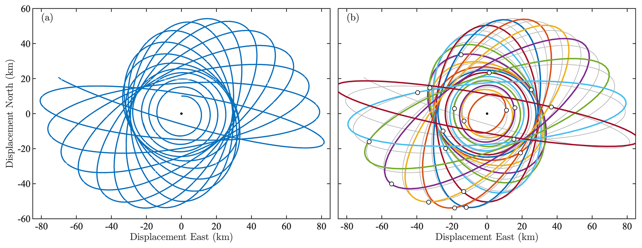
Figure 4A synthetically constructed modulated elliptical signal (a) together with (b) ellipses inferred from the analytic signal method. See text for details. The thin gray line in panel (b) is the same as the blue line in panel (a). Dots in panel (b) give the state of the signal at the moments at which the ellipses are shown; these are intersection points of the signal curve and the ellipses.
It is useful at this point to show an example. The signal in Fig. 4a is synthetically constructed from the ellipse generation equation, Eq. (1), with parameter choices given in Appendix A. This anticyclonically orbiting signal starts out circular for the first quarter of its duration, then transitions to a uniformly precessing ellipse ( constant, where the prime is a time derivative), with an increasing eccentricity or decreasing circularity , all the while linearly growing in amplitude κ(t) and also, though not apparent in this plot, in frequency. Using the analytic signal method discussed subsequently, one may assign a time-varying ellipse to this signal, snapshots of which are shown in Fig. 4b every 50 d beginning on the 25th day of this 1000 d time series. The ellipse properties so inferred, when themselves inserted into the generation equation, exactly reproduce the original signal.
To develop this method, we first turn to the case of a univariate signal. The modulated elliptical signal is a generalization to two dimensions of an amplitude-modulated and frequency-modulated univariate oscillation:
where ax(t)>0 is a time-varying, or instantaneous, amplitude and ϕx(t) is an instantaneous phase. Signals of this type include pure sinusoids, with ax(t)=ao and , as a special case, but are far more general. A simple example of a modulated oscillation is a wave packet. A wave packet exhibits amplitude modulation in the form of its envelope and possibly frequency modulation if the frequency content is not uniform over time. Nevertheless, it is also distinctly oscillatory. Equation (10) captures the essence of such oscillatory features that depart from being strictly sinusoidal.
Given x(t), one wishes to recover the ax(t) and ϕx(t) that could generate it via Eq. (10). That is, we wish to associate with x(t) an amplitude ax(t) and a phase ϕx(t), in order to conceptualize and describe x(t) as a modulated oscillation. The association of a physically meaningful amplitude and phase with a given signal is an underdetermined problem, as an infinite family of amplitude–phase pairs on the right-hand side can generate the observed signal on the left-hand side. However, a meaningful solution to this problem was found by Gabor (1946) in a landmark paper, by introducing what is now known as the analytic signal method; see, e.g., Picinbono (1997) and references therein for a more modern treatment.
In the analytic signal method, a particular amplitude–phase pair, known as the canonical amplitude and phase, are determined by pairing the real-valued signal x(t) with an imaginary part consisting of its own Hilbert transform,
where ℋ is the Hilbert transform operator defined as
with “” denoting the Cauchy principal value integral. The resulting complex-valued signal x+(t), the real part of which is the same as the original signal, , is called the analytic signal associated with x(t), or its analytic part. An analytic signal is by definition one whose Fourier transform vanishes on negative frequencies, as will shortly be seen to be the case for x+(t).
The canonical amplitude is defined uniquely in terms of the analytic signal by and the canonical phase function by . For the special case of a sinusoidal signal , the analytic signal is given by, as will be shown shortly,
Thus for a sinusoid, the amplitude and phase assigned using the analytic signal method agree with the obvious choices, i.e., ax(t)=ao and . This crucial property is known as harmonic correspondence (Vakman, 1996). The canonical phase can be differentiated to give the instantaneous frequency (Gabor, 1946; Picinbono, 1997),
which allows for the objective quantification of the time-varying frequency content of a modulated oscillation. See Lilly and Olhede (2010b) and references therein for a discussion of the close connection between the instantaneous frequency and the conventional definition of a mean frequency from first Fourier-domain moment of the spectrum of x(t).
2.4 Analytic signal details
To better understand the analytic signal, we first note that the Hilbert transform has a simple action in the frequency domain. Let X(ω) be the Fourier transform of x(t), from which x(t) is recovered using the inverse Fourier transform
One may show that the Hilbert transform of x(t) is given by (e.g., Papoulis, 1962, pp. 37–38)
where the signum function
returns the sign of its argument. The Hilbert transform thus simply changes the sign of Fourier coefficients for negative frequencies while lagging all Fourier phases by 90∘. It follows that the analytic signal can be written as
where is the unit step function. The analytic operator [1+iℋ] acts to double the Fourier coefficients of all positive frequencies while setting those of negative frequencies to zero. Thus, it renders a signal analytic.
Recall that a cosine and sine have the Fourier representations of
where δ(ω) is the Dirac delta function. From these, Eq. (16) shows that the action of the Hilbert transform is to decrement the phases of all sinusoidal components by 90∘, i.e., ℋcos (ωot)=sin (ωot) and . Harmonic correspondence, Eq. (13), then follows.
A compelling argument in favor of the analytic signal method is due to Vakman (1996); see also Huang and Yang (2011). Consider assigning a time-varying amplitude and phase by pairing the real-valued signal x(t) with some other imaginary part than its Hilbert transform. That is, in Eq. (11) we replace [1+iℋ] with [1+iℒ], where ℒ is some yet-to-be-determined linear operator. Vakman (1996) proves that the Hilbert transform ℋ is the only linear operator that leads to an amplitude and phase pair with the following three properties: (i) harmonic correspondence; (ii) amplitude continuity, meaning that small variations δx(t) of the signal x(t) should correspond to small variations δax(t) of the amplitude; and (iii) phase invariance to scaling, such that the instantaneous phase of x(t) and that of a rescaled signal cx(t), where c>0, should be identical. Vakman's conditions leave little choice but to accept that the analytic signal method is the natural way to solve this inverse problem.
Note that there are actually two different sets of amplitude–phase parameters: those used to generate a signal via the right-hand side of Eq. (10), which are unobservable, and the canonical amplitude and phase that are assigned to an observed signal using Eq. (11). Here we have used the same symbols to denote both sets in order to avoid a cumbersome notation. While both sets of parameters generate the same signal, and while they are guaranteed to be identical for the case of a sinusoidal signal by harmonic correspondence, in general, they need not be the same.
A condition for when the generating amplitude and phase are identical to the canonical amplitude and phase was found in a remarkable paper by Bedrosian (1963). The so-called Bedrosian condition for a real-valued univariate signal can be viewed as a type of slow variation condition, in which the frequency-domain support for the amplitude function ax(t) exists on strictly lower (that is, smaller magnitude) frequencies than the support of cos ϕx(t). Broadly speaking, the difference between the generation parameters and the canonical parameters is expected to become larger as the strength of modulation specified by the generation parameters increases.
2.5 Inferring ellipse properties
The analytic signal method of assigning a time-varying amplitude and phase to a univariate signal x(t) was generalized to the multivariate signals by Lilly and Olhede (2010b), which we will simplify and build on in this section. In vector notation, the ellipse generation equation, Eq. (1), becomes
where R(ϑ) is the rotation matrix through some angle ϑ,
The analytic version of the bivariate signal x(t) is given by
in terms of which the canonical ellipse parameters may be defined via
This assignment is readily verified to satisfy harmonic correspondence for the special case of a sinusoidal ellipse with fixed geometry, that is, with a(t)=ao, b(t)=bo, θ(t)=θo, and .
To infer the ellipse parameters from x+(t), it is convenient to use a set of matrices introduced by Lilly (2018). Define
where is recognized as the 90-degree counterclockwise rotation matrix, and K and L are the reflection matrices about the lines y=0 and x=y, respectively. K and L are found to transform under rotations by some angle ϑ as
as shown in Lilly (2018), with the superscript “T” denoting the matrix transpose.
Using for convenience κ(t) and ξ(t) rather than a(t) and b(t), one finds that the definition in Eq. (24) implies
for the values of the canonical ellipse parameters expressed in terms of the analytic signal x+(t). Here “H” is the Hermitian or conjugate transpose, is the norm of some vector x, and we have made use of the rotation formulas, Eqs. (26) and (27), in the expression for θ(t). Finally
recovers the semi-axes lengths from κ(t) and ξ(t), as are obtained by inverting Eq. (5).
Equations (28)–(31) will be called the ellipse inversion equations, in the sense of going backwards from an observed signal to ellipse parameters. These expressions are more direct than those given in Lilly and Gascard (2006) and Lilly and Olhede (2010b), which use the rotary amplitudes and phases as an intermediate step in the inversion. Returning to the synthetic example, grouping the x(t) and y(t) signals shown in Fig. 4 into a vector x(t)=[x(t) y(t)]T, taking its analytic part, and inserting the result into the inversion equations, Eqs. (28)–(31), leads to the ellipses in Fig. 4b.
As in the case of a univariate signal, there is a distinction between the generating and the inferred, or canonical, ellipse parameters, both of which lead to the same time-varying ellipse. These sets of parameters are identical for a sinusoidally orbited fixed ellipse and are expected to become increasingly different as the modulation strength increases. Further examination of the conditions for exact recovery of the generating ellipse parameters is outside the scope of this paper.
The generalization of the univariate instantaneous frequency, Eq. (14), to the multivariate case is called the joint instantaneous frequency
as introduced by Lilly and Olhede (2010b). For the case of a bivariate signal this can be rewritten as
which is seen to be the power-weighted average of the x- and y-component instantaneous frequencies. Note that this definition of ω(t) implies that it will generally be positive and that its power-weighted integral is guaranteed to be non-negative. This is most apparent from its frequency-domain form; see Eqs. (48) and (50) in Lilly and Olhede (2010b).
The bivariate instantaneous frequency can be written in terms of the ellipse parameters as (Lilly and Olhede, 2010b)
and thus involves contributions from the rates of change of both the phase ϕ(t) and the orientation angle θ(t). Variations in ϕ(t) correspond to a particle orbiting a fixed ellipse, while variations in θ(t) capture the precession of the ellipse itself.
In the previous section, it was shown that given a trajectory consisting of only a single modulated elliptical signal, a unique assignment of time-varying ellipse parameters that could have generated it may be found by forming the associated analytic signal. Real-world eddies, however, do not occur in isolation, but rather they are superposed onto flows due to large-scale turbulence, other eddies, waves, and any self-propagation tendency of the eddy itself. To adapt the analytic signal method to handle realistic trajectories, we therefore need to incorporate a filtering step. This is accomplished using the continuous wavelet transform, as described next. We remind the reader that the notation list in Table A1 is available as a resource.
3.1 A model for Lagrangian trajectories
A Lagrangian instrument records a time-varying longitude Θ(t) and latitude Φ(t), both taken to be in radians. For small deviations about some fixed point (Θo,Φo), the trajectory can be locally approximated as
where x(t) and y(t) are the east–west and north–south displacements in a plane tangent to the Earth at (Θo,Φo) under the small angle approximation, and R⊕ is the mean radius of the Earth. For trajectories lying within a small domain such as the Gulf of Mexico, the errors on estimated eddy properties resulting from neglecting the full spherical geometry are quite minor. The Coriolis frequency corresponding to latitude Φ(t) is , where rad s−1 is the Earth's angular rotation rate.
The displacement signal x(t) is assumed to be composed of two portions:
with the being modulated elliptical signals of the form given in Eq. (21) and xϵ(t) being a background displacement field that will be described as a stochastic process. The modulated oscillations capture the displacement of a particle orbiting the center of a possibly elliptical eddy, as well as the motion of particles within inertial oscillations, while the background xϵ(t) represents motions due to such processes as geostrophic turbulence and the wind-forced flow, as well as translation due to a possible mean flow or systematic drift, and finally any measurement noise.
The corresponding model for the latitude and longitude signals is
Here and are respectively latitude and longitude deviations associated with the modulated oscillations, related to via small-angle expansions as in Eq. (37). The combination ℑ{log eiϑ} accounts for the case in which the longitude crosses the antimeridian at ±π. Note that Eq. (39) would require modification for trajectories in the vicinity of the poles.
Each of the modulated oscillations is nonzero only over a continuous interval within the time window over which x(t) is defined. The total number of oscillatory components present in a time series is denoted by M⋆, which may be zero, one, or more than one. The number of nonzero oscillatory components present at any one time is an important quantity , referred to as the multiplicity. As with M⋆, the multiplicity M(t) may be zero, one, or more than one at each time. Examples in which the multiplicity M(t) is equal to 2 are an eddy superposed on an inertial oscillation or an eddy advected by another eddy.
The conceptual model of Eq. (38) is an example of an unobserved components model (e.g., Nerlove, 1967; Harvey, 1989), meaning that one believes the observations to be the sum of several components which cannot be observed individually but only as part of an aggregate process. We may refer to the as latent oscillations, in the sense of being present but obscured. The goal of this section is present a method for extracting, as accurately as is possible, oscillatory displacement signals associated with coherent eddies from an observed trajectory x(t) in the presence of a background flow xϵ(t) and then to link these displacements to the physical properties of eddies.
3.2 A motivational example
The analytic signal method presented in Sect. 2 is intended for the case in which only a single modulated oscillation, and nothing else, is present in a time series. It is not intended to work in the case of a composite signal such as in the unobserved components model of Eq. (38) and performs poorly in such cases.

Figure 5Panel (a) shows the signal from Fig. 4a, modified through the addition of a uniform westward drift together with a stochastic component. The sum of the westward drift and the stochastic component is the red curve, which defines the moving center for the modulated elliptical signal. Panel (b) presents ellipses inferred using the wavelet ridge method. The thin black line in both panels is the estimated background displacement curve from the wavelet ridge analysis, an estimate of the red curve in (a).
To illustrate this, and to motivate the approach developed in this section, we return to synthetic signal shown in Fig. 4a. We write with the synthetic signal chosen to be x⋆(t) and set the background process xϵ(t) to consist of a uniform westward drift at 0.5 cm s−1 plus a stochastic component. The latter has a red velocity spectrum with a velocity standard deviation of 0.25 cm s−1, constructed as described in Appendix A. The sum of the westward drift and stochastic displacement forms xϵ(t), shown as the red line in Fig. 5a. The full signal x(t) is the blue curve in Fig. 5a.
Applying the analytic signal method of the previous section to a detrended version of the total displacement signal x(t), one obtains the ellipses shown in Fig. 6a. Even though the stochastic signal is small compared to the oscillatory signal, the inferred ellipses are nothing like those we found earlier in Fig. 4b. The reason is that the analytic signal method treats the entire time series as an aggregate, lumping the stochastic signal together with the oscillation. By contrast, the ellipses inferred using the wavelet-based method, developed subsequently and shown in Fig. 6b and also in Fig. 5b, are very close to those seen earlier in Fig. 4b for the analytic signal method applied to the isolated oscillatory signal. The wavelet-based method essentially combines the analytic operator with an adaptive filtration, minimizing, though not entirely removing, the influence of the other variability.
3.3 Wavelet analysis basics
The extraction of unobserved modulated elliptical signals from the observed position signal x(t) can be accomplished using a method called multivariate wavelet ridge analysis (Lilly and Olhede, 2009a, 2012a). This is a generalization to multiple time series of the wavelet ridge analysis method introduced by Delprat et al. (1992), which was extended and refined by Mallat (1999) and later by Lilly and Olhede (2010a). The starting point of wavelet ridge analysis is the choice of a family of oscillatory, time-localized functions, called wavelets, that will serve as the basis for detecting modulated oscillations. The choice of a suitable wavelet function, conventionally denoted ψ(t), involves a tradeoff between time resolution – the ability to resolve sudden changes in an oscillatory signal – and frequency resolution, the ability to distinguish between variability in different frequency bands.
Systematic examination of continuous-time wavelets in common use by Lilly and Olhede (2009b, 2012b) pointed to the generalized Morse wavelets (Daubechies and Paul, 1988; Olhede and Walden, 2002) as an ideal wavelet family, encompassing all other commonly used forms. These are defined in the frequency domain as
where is again the unit step function, β and γ are two controlling parameters, and aβ,γ is a normalizing constant defined as
for reasons to be seen shortly. The time-domain wavelets ψβ,γ(t) are given in terms of Ψβ,γ(ω) via the inverse Fourier transform,
On account of the unit step function in Eq. (41), these wavelets have vanishing support at negative frequencies and are therefore said to be analytic.
The frequency at which Ψβ,γ(ω) obtains its peak magnitude is readily found, from differentiating Eq. (41), to occur at , called the peak frequency. Another key quantity is the normalized curvature of the wavelet at the peak frequency (Lilly and Olhede, 2009b),
The frequency-domain wavelets can be approximated in the vicinity of their peak frequency as a Gaussian:
as shown in Lilly and Olhede (2012a); here fβ,γ(ω) is a deviation function, the form of which is given in that reference. plays the role of the standard deviation and is consequently a nondimensional measure of the frequency-domain width of the wavelets about their peak frequency. Pβ,γ itself is therefore a nondimensional measure of the wavelet temporal width. Lilly and Olhede (2009b) show that is roughly the number of oscillations spanned by the central portion time-domain wavelet, defined as .
With γ held fixed, β controls the time–frequency tradeoff. Increasing β increases the number of oscillations in the wavelet, decreasing the temporal resolution but increasing the frequency resolution. As to the choice of γ, Lilly and Olhede (2009b, 2012b) find that the γ=3 wavelets are nearly symmetric about their peak in the frequency domain, nearly Gaussian in their frequency-domain shape, and have a standard measure of time–frequency concentration – the Heisenberg area – that is nearly optimal for fixed β and any γ. On account of these desirable properties, the γ=3 wavelets are recommended for general use, and we will follow that recommendation here.
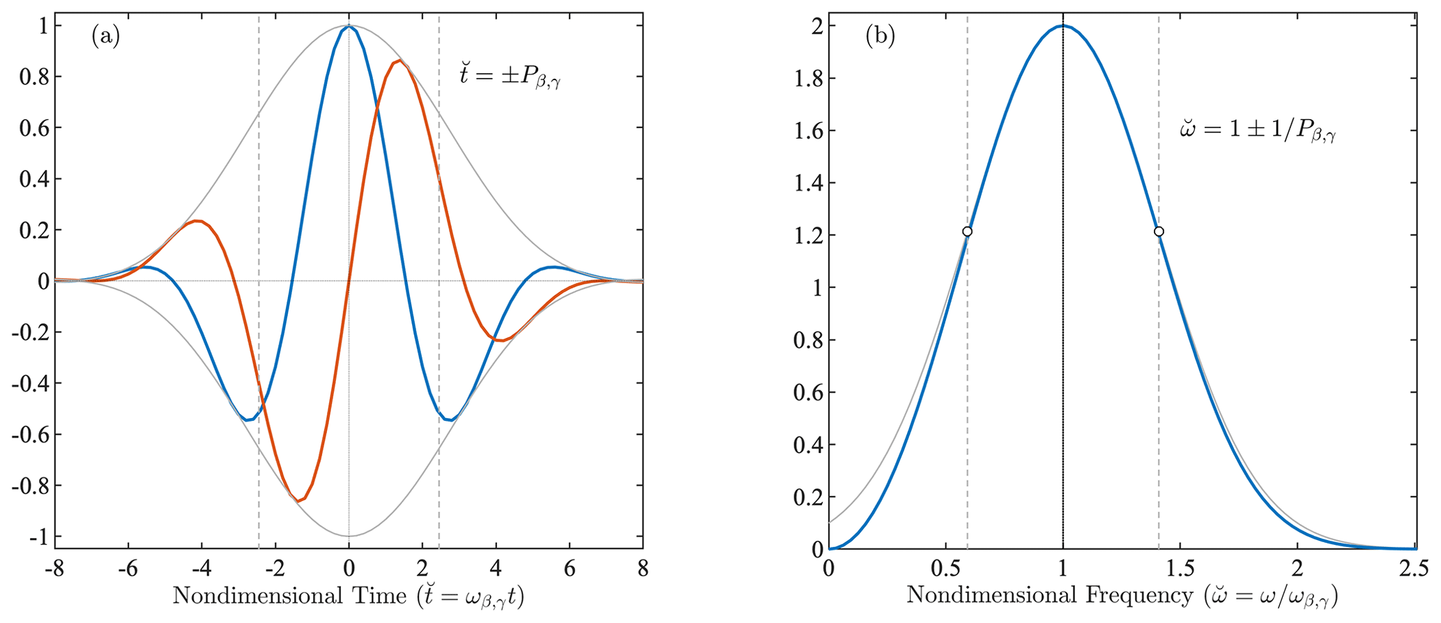
Figure 7A generalized Morse wavelet ψβ,γ(t) with the choice in (a) the time domain and (b) its Fourier transform Ψβ,γ(ω). Both time and frequency have been nondimensionalized, as and , respectively. In panel (a), the blue and orange lines are the real and imaginary parts, respectively, of , while the thin gray lines are plus or minus the wavelet modulus . Here the time-domain wavelet has been rescaled to have unit amplitude. In panel (b), the thin gray line is the Gaussian approximation in Eq. (45). Vertical dashed lines in both panels are measures of the wavelet half-width based on Pβ,γ, as described in the text, while dots in (b) are the wavelet value at . Dotted lines mark and zero magnitude in (a), and the wavelet peak frequency of in (b).
The generalized Morse wavelet we will use in this paper, β=2 and γ=3, is shown in Fig. 7. Here time and frequency have been rescaled, with and , such that the peak frequency occurs at . This is a quite time-localized wavelet, with at most only two full oscillations visible in the time domain. In the frequency domain, we see that the Gaussian approximation, Eq. (45) with the deviation term fβ,γ(ω) neglected, is a good approximation to the wavelet and is indistinguishable from it in a broad region around the peak. The frequencies correspond to 1 standard deviation of the Gaussian about the peak, values at which the exponential in Eq. (45) is equal to . In the time domain, we see slightly less than one full oscillation within the window , in agreement with being the number of oscillations within the central window.
Next we use many rescaled versions of the wavelet to filter a univariate signal x(t), leading to the wavelet transform
where the asterisk denotes the complex conjugate, with s being called the scale. The scale s transform amounts to a complex-valued bandpass centered on the rescaled wavelet peak frequency and thus filters oscillations having a period in the vicinity of . Here we use the scale normalization for the wavelet transform, following Lilly and Olhede (2009b). Note that the important dependence of the transform on the controlling parameters of the wavelet, β and γ, is suppressed to avoid cumbersome notation. However, it is important to bear in mind that the wavelet transform is not an intrinsic property of a time series. Rather, it is a joint function of a time series and a particular wavelet.
In the frequency domain, the wavelet transform can be expressed as
on account of the convolution theorem. This is derived by substituting into Eq. (46) the inverse Fourier transforms of the signal and the wavelet, Eqs. (15) and (43) respectively4. Due to the analyticity of the wavelets, the lower limit of integration may be set to zero. From this expression one sees that wx(t,s) consists of a set of versions of x(t) that have been bandpassed using rescaled wavelets, Ψβ,γ(sω), as the bandpass filters. It is also clear that the wavelet transform using an analytic wavelet is itself analytic, i.e., supported only on non-negative frequencies, for any fixed scale s.
With these definitions, the wavelet transform of a phase-shifted sinusoid
is found to be
using Eq. (47) together with Eq. (19). We see that wo(t,s) obtains its maximum magnitude at the scale . Moreover, if one chooses a normalization such that the maximum value of the wavelet is , we have
such that the wavelet transform at the maximizing scale recovers the analytic version of the signal xo(t). Owing to the choice for the normalizing constant in Eq. (41), we have as desired.
3.4 Oscillation detection using wavelet ridge analysis
Turning now to a vector-valued signal x(t), its wavelet transform will be a vector-valued function of time and scale,
A ridge of this vector-valued wavelet transform w(t,s) is a time-varying scale curve along which
such that marks a local maximum of the wavelet transform magnitude with respect to variations in scale s. This is the multivariate ridge definition introduced by Lilly and Olhede (2009a, 2012a), building on earlier work on univariate wavelet ridge analysis by Delprat et al. (1992), Mallat (1999), and Lilly and Olhede (2010a). It was shown by Lilly (2017) that a ridge can be interpreted as a maximum with respect to scale of the local signal energy density, or power; see Section 2(c) therein. The principle of wavelet ridge analysis is therefore not one of minimizing an error, but rather of maximizing the power of a projection.5
For a vector-valued signal with only a single modulated oscillation present, , it can be demonstrated that a wavelet ridge approximates the location of the instantaneous frequency curve ω(t), that is,
while the analytic signal associated with x(t) is approximately recovered by simply taking the value of the wavelet transform along the ridge,
These equations are derived in Lilly and Olhede (2012a), their Eqs. (86) and (61) respectively, wherein the explicit forms for next-order terms in the approximations are given. Those terms, omitted for brevity here, represent errors in the wavelet ridge method arising from the strength of the modulated oscillation itself and therefore are a type of bias error. Such errors vanish when the modulation strength vanishes, that is, for the case of a sinusoidal signal.
When applied to a real-world signal x(t), wavelet ridge analysis leads to a set of ridges, , the corresponding estimated oscillations , their associated ellipse parameters , , , and , and finally the instantaneous frequencies , for . Here is the total number of ridges present after applying any editing criteria, such as that discussed in the next subsection. These estimates are interpreted here in the context of the unobserved components model, Eq. (38). We would say that the ridges provide estimates of latent oscillations that appear to be present in the time series, with being an estimate of the total number M⋆ of such components. The dependence of all of these estimates on the wavelet properties (β,γ) is implicit.
Application of the ridge analysis method to surface drifter trajectories leads to another type of error, namely false positives arising from the stochastic background xϵ(t). As discussed in the Introduction, the ridge analysis will identify some events that, rather than corresponding to latent oscillations that are actually present, arise by chance due to the interaction of the wavelets with the background. These are a major problem because they mean a certain fraction of detected ridges would be expected to be entirely spurious. A means of addressing the false positives is presented in Sect. 4.
If the multiplicity exceeds unity, we may define the time-varying position of the center of the mth oscillation as
which is the difference between the full displacement signal and the displacement signal associated only with that ridge. This quantity is estimated by . To put this in terms of latitude and longitude, we first convert and into the estimated deviations
where Φo is latitude of the reference point that was used to create the Cartesian vector x(t) from latitude and longitude in Eq. (37). Then
gives the estimated latitude and longitude position of the center of the mth oscillation.
Finally, the background process on the Cartesian plane, xϵ(t), is estimated by summing over all ridges and forming the residual
The corresponding latitude and longitude signals, and , are formed by subtraction after inserting the estimated deviations and into Eqs. (39) and (40).
For notational convenience, we will henceforth drop the superscripts “m” on ridge quantities, letting it be understood that they pertain to a particular latent oscillation.
3.5 A ridge length threshold
Experience shows that it is important to set a threshold for the minimum length of a ridge. The ridge length is measured in terms of the number of oscillations executed along the ridge, which is found by integrating the estimated instantaneous frequency :
from the initial time point of the ridge ti to its final time point tf. Note that L is nondimensional. For a constant instantaneous frequency, , observed over a time interval of duration , we have , which is the number of periods executed over time interval T.6
A threshold on L is found to be important for two reasons. Firstly, when any kind of noise is present, the random generation of false positives becomes more common as the ridge length decreases; thus L is important for assessing statistical significance, as will be seen in more detail shortly. Secondly, as the ridge length becomes small compared to the number of oscillations experienced by the wavelet, the very idea that the wavelet transform is illuminating some aspect of the time series becomes suspect. For ridges comparable to or shorter than the length of the wavelet, isolated noise points or minor discontinuities in the time series lead, via the convolution theorem, to copies of the wavelet itself being presented in the wavelet transform. As mentioned earlier, the wavelet transform is a joint function of the wavelet and the signal; ridges comparable to or shorter than the wavelet duration tend to be features arising from the former.
A ridge length threshold is therefore employed in which we keep only ridges with lengths
for some choice of n, where is approximately the total number of oscillations spanned by the wavelet. We will set n=1 so that for the β=2 and γ=3 wavelet used herein, a choice that we find sufficient to eliminate obviously spurious features.
3.6 A synthetic example
As a simple example, the wavelet ridge analysis for the synthetic composite signal from Fig. 5 is shown in Fig. 8, using the ψ2,3(t) wavelet from Fig. 7 and the ridge length criterion . The white and black lines denote ridge curves . A clear maximum of the wavelet transform magnitude ∥w(t,s)∥ with respect to scale is observed, marked by the heavy black line. The white lines are short ridges marking minor, generally indiscernible maxima of the wavelet transform. These are spurious features arising randomly due to the stochastic background process xϵ(t) and are rejected based on the ridge length criterion. After this rejection, only the black curve remains. Thus the wavelet ridge analysis supports the unobserved components model with a multiplicity of 1, , and we interpret the sole remaining ridge as an estimate of the latent oscillatory signal x⋆(t).
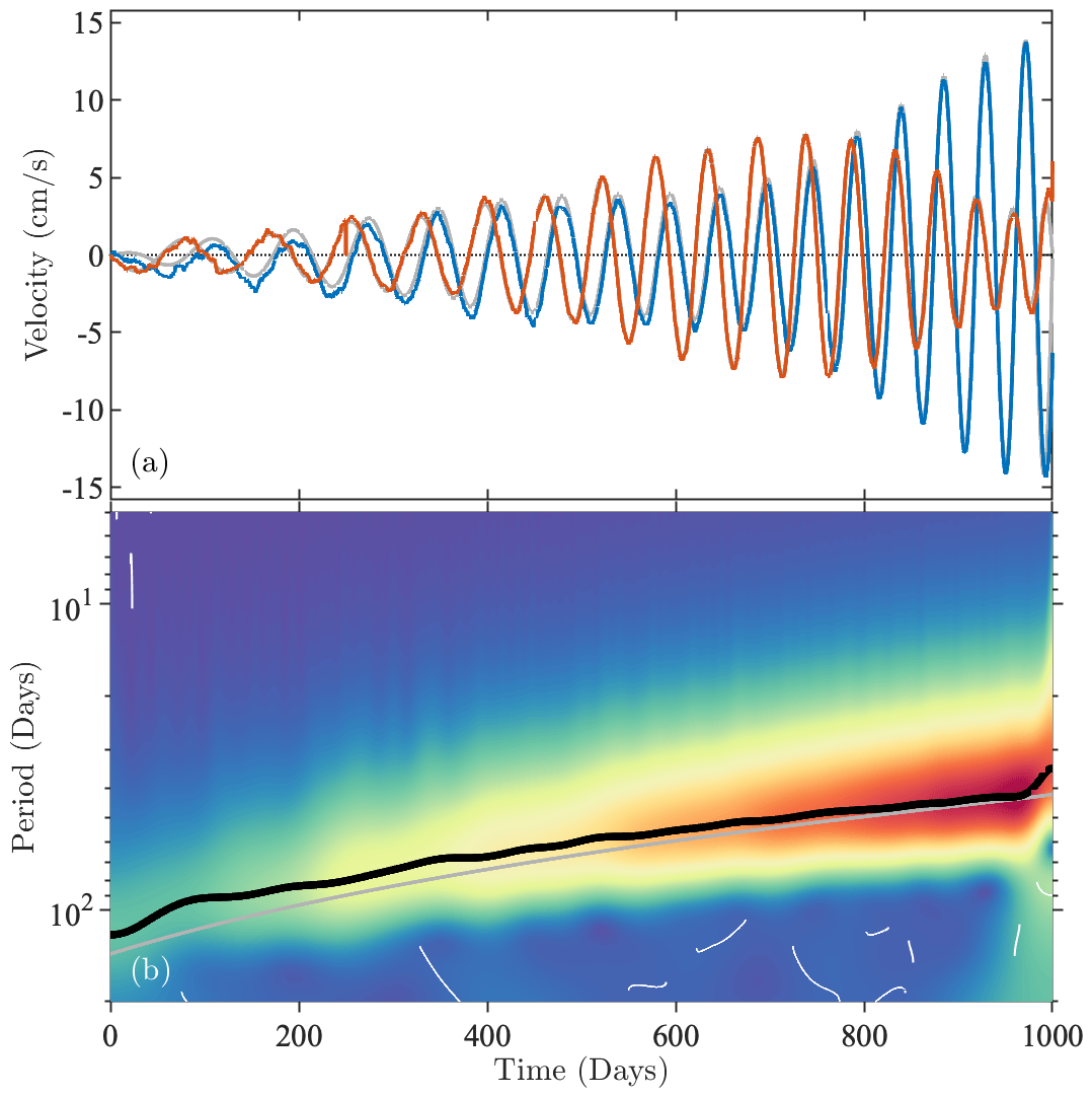
Figure 8Multivariate wavelet ridge analysis applied to the synthetic composite signal shown in Fig. 5a. Panel (a) is the velocity corresponding to the displacement signal, with blue for the eastward component and orange for the northward component. The magnitude of the wavelet transform ∥w(t,s)∥ of the displacement signal using a generalized Morse wavelet is shown in (b), with the heavy black curve denoting a major ridge and the white curves denoting short, spurious ridges arising as a result of the stochastic background process. The period corresponding to the generating parameters is shown as the gray line; see Appendix A. The gray lines in panel (a) are the velocity components formed by differentiating the ridge-based estimate of the oscillatory displacement signal that is found as the real part of Eq. (54); these are very close to the original signal and are not visible for most of the record because they are overplotted by the blue and orange curves.
Evaluating the wavelet transform along this ridge curve as in Eq. (54) leads to an estimate of the analytic signal vector associated with the latent oscillation x⋆(t). Application of the ellipse inversion equations, Eqs. (28)–(31), then gives the estimated ellipses shown in Figs. 5b and 6b. Taking the real part of this estimated analytic signal produces an estimate of x⋆(t) itself, , the gray line in Fig. 6b, with its corresponding estimated velocities shown in Fig. 8a as gray lines. Subtracting the estimated oscillation from the full signal leads to the estimated background, , the black line in Fig. 5a and b.
It is clear from Figs. 4–6 that the wavelet ridge analysis does an excellent job of extracting the true oscillation x⋆(t) from the composite signal x(t), effectively stripping out the background process xϵ(t). Note that this signal, like realistic eddy signals, exhibits substantial frequency modulation, and thus Fourier-based or narrowband methods such as bandpassing or complex demodulation would not be suitable.
Importantly, we have not needed to specify any properties of the oscillatory signal apart from the frequency range of the transform. As mentioned earlier, Lilly and Olhede (2009b, 2012b) have established the sensibility of the choice γ=3 based on symmetry considerations; thus the only free parameter of the wavelet transform is β, which controls the number of oscillations in the wavelet. The choice of β, it should mentioned, encodes an implicit tradeoff between resolving temporal variability of detected modulated oscillations and separating an oscillation from neighboring variability in the frequency domain. Smaller values of β are more suitable for signals exhibiting strong temporal modulation, whereas large values would be more appropriate if it were necessary to resolve closely spaced oscillations in frequency. The β=2 value used here, corresponding to quite narrow wavelets in the time domain, appears to be suitable for this and many other Lagrangian datasets.
3.7 One-sided ridges
Because here we are particularly interested in eddies, which tend to be destroyed if strained to a high degree of eccentricity, a modification is made to the ridge analysis. In its general form, the ridge analysis places no constraints on the polarization, that is, the degree of eccentricity of the signal. Numerical experiments with noise datasets show that when ridges emerge, they can be of any polarization, and this polarization tends to wander with time, sometimes even changing sign across ξ(t)=0 as the ridge switches from being dominated by positive rotations to dominated by negative rotations. Such transitions are not realistic for real-world eddies, and permitting them in the ridge analysis leads to a greater number of false positives which must be sorted out later.
It therefore seems preferable to explicitly exclude sign transitions across ξ(t)=0. Such ridges will be said to be one-sided and are formed as follows. The Cartesian wavelet transforms are converted into a pair of rotary transforms as
with giving the local magnitude of positive oscillations in , and giving the magnitude of negative oscillations; see, e.g., Lilly and Gascard (2006). As this matrix transformation is unitary, we have . We then form , the difference of the positive and negative rotary wavelet transform amplitudes.
The wavelet ridge analysis is then performed twice. Ridges of w(t,s) are first found after masking out regions where and then again after masking out regions where . Each of these two sets of ridges lacks sign transitions. Before applying the ridge length threshold, Eq. (61), the union of these two sets of ridges contains the same ridge points as the full set of ridges, with the exception of any ridge points for which Δw(t,s) is exactly zero. After applying the ridge length cutoff, the set based on the one-sided ridges will be smaller than the full set, because sign transitions are essentially treated as ridge endpoints.
The net result of this modification is that ridges lacking a sign transition are unchanged, ridges containing sign transitions are broken into shorter segments, and fewer spurious, false positive events survive the ridge length threshold. A desirable feature of this approach is that it does not involve setting an ad hoc threshold on the degree of eccentricity, as any numerical value of the circularity ξ(t) may still be detected provided the rotation sense does not reverse.
In this section the wavelet ridge analysis method is applied to the Gulf of Mexico drifter dataset presented in Fig. 1. Issues of false positives are addressed, leading to an edited eddy dataset where such features are believed to be rare. Note that in this section we omit the “m” superscripts on modulated oscillation and ridge quantities to avoid excessive notation.
4.1 Choice of frequency band
The first decision to be made is what band of scales, or frequencies, the wavelet transform should be performed over. The instantaneous frequency ω(t) can be nondimensionalized relative to the Coriolis frequency at the center of an oscillation, , as
which we construct to be a signed quantity, positive for cyclonic motion and negative for anticyclonic motion. We choose to carry out the ridge analysis within a time-varying frequency band such that the nondimensional instantaneous frequency is in the broad range . This range is expected to capture eddy-related motions from slow circling on the far flanks of large eddies, up to the rapid oscillations within highly nonlinear submesoscale eddies.
It is helpful to examine the physical interpretation of the nondimensional instantaneous frequency ω*(t) by referring to the special case of a steady circular eddy with azimuthal velocity profile vθ(r). This eddy has vertical vorticity ζ(r) and angular velocity ϖ(r) profiles given by
with being the vertical unit vector. Particle paths about the eddy center at some fixed radius ro have solutions given by . Thus for the case of constant angular velocity in a circular eddy, the angular velocity is the same as the signed instantaneous frequency, ϖ(ro)=sgn(ξ(t))ω(t).
Let the eddy have a maximum azimuthal velocity at radius Ro with a value of Vo=vθ(Ro). Its nonlinearity may be measured through the vortex velocity Rossby number,
see, e.g., D'Asaro et al. (1994). (Note that the function of time arises because in this simple kinematic model we permit – unrealistically – the fixed eddy to move meridionally without adjustment.) One may extend the vortex Rossby number to measure the local nonlinearity of the flow at each radius via
The equalities on the right-hand side show that for a steady circular eddy, the local velocity Rossby number RoV(r,t) is twice the nondimensional instantaneous frequency ω*(t) that would be observed for a particle located at radius r.
Another measure of the bulk nonlinearity of an eddy is its vorticity Rossby number, defined as
with ζo being the vertical vorticity averaged over the radius Ro. In the case that the eddy core is in solid-body rotation, then vθ(r)=αr for some constant α with r≤Ro, and the core vorticity is from Eq. (64). It follows that Roζ and RoV are identical for solid-body rotation.
If a time-varying lower boundary is set for the ridge frequency band at , it is believed on dynamical grounds that no anticyclonic eddies will be missed and also that inertial oscillations will be entirely excluded, as we now show. It is well known that for anticyclonic, circular, barotropic eddies, there is a stability boundary at ; see Kloosterziel (2010) for a very useful historical discussion. Eddies having more negative values of relative vorticity would experience a type of instability known as inertial or centrifugal instability. Consequently such eddies are not observed in nature, with the most intense documented anticyclones, such as the Lofoten Basin Eddy (e.g., Søiland and Rossby, 2013; Bosse et al., 2019; Trodahl et al., 2020), having vorticities of around . This stability boundary corresponds to a nondimensional frequency of .
Inertial oscillations typically occur at a Fourier frequency of or , with the negative sign indicating that inertial oscillations turn clockwise in the Northern Hemisphere and counterclockwise in the Southern Hemisphere. However, in the presence of background vorticity, inertial oscillations experience a frequency shift (Kunze, 1985) from to . For the most extreme possible anticyclonic eddy at the stability boundary , assuming solid-body rotation, the shifted inertial frequency would then occur at or , the same frequency as the eddy itself. Thus inertial shifting in an anticyclone brings the inertial oscillation frequency away from f and closer to the eddy frequency, and these become identical for the most nonlinear anticyclones at .
Therefore, both to avoid inertial oscillations and because no eddies are physically expected, the ridge analysis should be truncated to exclude events below the time-varying curve . Yet since there is no corresponding stability boundary on the cyclonic side, one should anticipate the possibility of intense cyclonic eddies exceeding . The truncation to will therefore be done at a later stage once we scrutinize the initial results using the symmetric frequency band .
4.2 An example from the Bay of Campeche
An example of applying the one-sided ridge analysis to a drifter trajectory from the Bay of Campeche in the southwestern Gulf of Mexico is presented in Figs. 9 and 10. The trajectory is shown in Fig. 9a, its latitude time series is the blue line in Fig. 9b, and its zonal and meridional velocities are presented in Fig. 10a. The trajectory has a complex oscillatory behavior, executing orbits that appear significantly non-circular, sometimes even square, and with numerous small cusps or loops. The latitude signal and velocity time series both reveal substantial nonstationarity, with a transition from low-frequency variability to higher-frequency variability around year day 50 of 2013, and to still higher-frequency variability around year day 110. The roughness observed in both position and velocity is suggestive of superposed variability from smaller temporal scales.
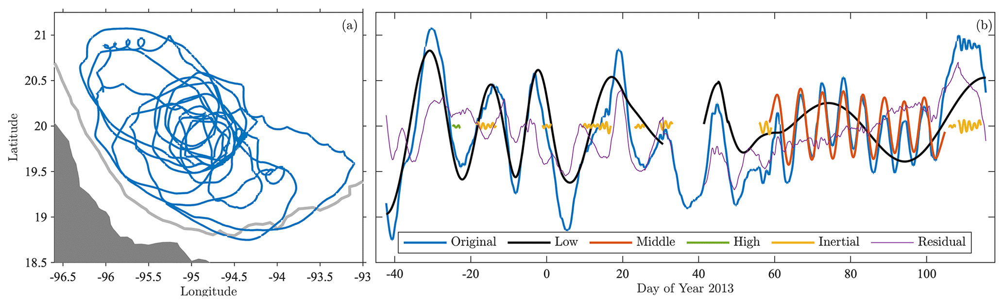
Figure 9An example of a trajectory decomposed according to the unobserved components model of Eq. (38), using the one-sided wavelet ridge method. Panel (a) shows the trajectory of drifter ID #80348 from the SGOM experiment, in the Campeche Gyre in the southwestern Gulf of Mexico. The dark gray shading is the continent and the thick light gray line is the 500 m isobath, as in Fig. 1. In panel (b), the original latitude signal of this trajectory is shown, along with oscillatory signals extracted from low, medium, and high frequencies, as well as the inertial band. Also shown is the residual after adding up all the extracted signals and subtracting the result from the original, Eq. (59), converted back to a latitude. The origins of the various curves are shown in Fig. 10.
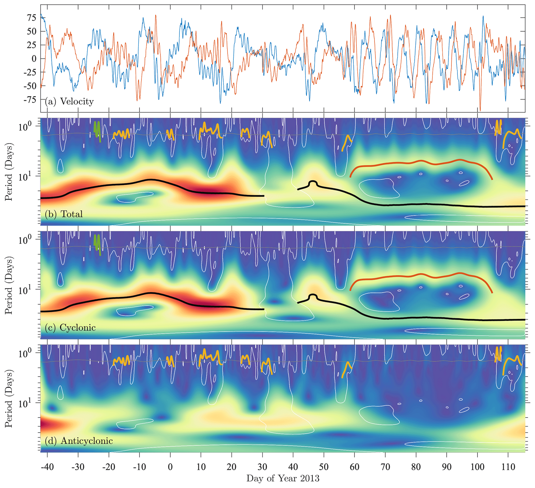
Figure 10One-sided wavelet ridge analysis of the signal presented in Fig. 9a. In (a), the zonal and meridional velocities vx(t) and vy(t) associated with the displacement signal from Fig. 9a are shown as blue and orange curves, respectively. Panel (b) shows the total wavelet transform magnitude, , while (c) and (d) show the magnitudes of the positive (or cyclonic) and negative (or anticyclonic) rotary transforms, and . The y axis in panels (b)–(d) is scale converted to oscillation period, . The thin, nearly horizontal gray line in panels (b)–(d) marks the time-varying Coriolis period , while the thin white lines are curves where the magnitudes of the two rotary transforms are equal, . The colored lines show all detected ridges of using the same color scheme as in Fig. 9b. There are two sets of ridges: those detected in when the positive rotary transform dominates and those detected in when the negative rotary transform dominates. To show their different origins, the ridges are superposed on the dominant transform as well as being drawn on the total transform . A condition of the one-sided algorithm is that the ridges terminate when they encounter the thin white lines, prohibiting transitions in rotation sense.
This trajectory is analyzed using the same generalized Morse wavelet employed previously. The range of scales in the transform is chosen to encompass the nondimensional frequency range for all latitudes within the Gulf of Mexico. The total transform magnitude , positive rotary transform magnitude , and negative rotary transform magnitude are shown in Fig. 10b–d. The colored lines in Fig. 10b–d are all the one-sided ridges – that is, scale curves satisfying Eq. (52), yet lacking sign transitions of – subject to the minimum ridge length of . Each ridge is drawn on the rotary transform that is dominant over its duration, as well as on the total transform in Fig. 10b. The one-sided ridges are not permitted to cross the white lines, which mark the locations at which .
The nonstationarity and multiscale variability that are apparent by eye are seen explicitly in the wavelet transforms. Small-scale variability is frequently attributable to inertial oscillations, as well as to a brief high-frequency cyclonic event around year day −22. At lower frequencies, a bifurcation is seen around year day 58, where a low-frequency cyclonic ridge splits into two cyclonic ridges: one that descends to lower frequencies and one that rises to higher frequencies. Whereas the higher-frequency member of this pair is visible by eye in the velocity and position time series, the lower-frequency member is not. The two low-frequency ridges that together span most of the record are notable for having relatively high values of eccentricity, unlike the middle-frequency ridge in the year day range 58–105, which is seen to be strongly circularly polarized in the cyclonic sense.
The contributions of the various ridges to the latitude variability are seen in Fig. 9b, after converting the ridges to latitude deviations using Eq. (56), as is the latitude residual . Oscillatory variability in the residual is much reduced compared with the original, particularly during the latter portion of the record dominated by the middle-frequency ridge. An exception is in the middle of the record, in the vicinity of the gap between the two low-frequency ridges, where the dominant wavelet polarization is observed to briefly change sign for a reason that is not readily apparent.
This complex trajectory is a good example of a situation in which the multiplicity – the apparent number of modulated oscillations at any moment – is greater than unity. The presence of inertial oscillations superposed on a background eddy, which accounts for the small cusps seen in Fig. 9a, is fairly common in this dataset. The superposition of two lower-frequency ridges, seen during year days 60–110, on the other hand, occurs rarely. A physical hypothesis consistent with these two ridges is that a particle is trapped in an eddy that is itself being advected by another eddy, with the lower-frequency signal arising from advection on the exterior flank of the second eddy. The superposition of these two signals accounts for the “wobble” in Fig. 9a, where the center of the tight loops in the middle of the plot appears to vary over time.
During the second half of the record, the sum of three oscillations – two eddy-like signals and an inertial signal – accounts for most of the variability apart from an over northward drift. This indicates that the unobserved components model of Eq. (38) can generate quite complex and irregular trajectories. During the first half, however, the residual curve exhibits more irregular oscillations, suggesting that during this time period the variability is less well matched to our proposed model. The more irregular behavior of the oscillation that dominates during this time period is suggestive of a particle that is weakly trapped on the flanks of the eddy rather than within its solid-body core. In this example, we have specifically chosen to investigate a complex signal; most of the detected signals are considerably simpler.
4.3 A noise dataset for a null hypothesis
Because the eddies we are interested in studying do not occur in isolation, but are embedded within a turbulent background flow, it is necessary to take into account that the background flow itself may occasionally, by chance, give rise to features in the drifter trajectories that appear as modulated oscillations. Such features would be detected by the ridge analysis and therefore constitute false positives.
To address this issue, we will compare the results of the ridge analysis to the results of a parallel analysis applied to a stochastic or “noise” dataset. The noise dataset will be created to match key properties of the observed dataset, but lacking the explicit signatures of any eddies. This will act as a null hypothesis and enable a level of statistical significance to be determined. It amounts to an idealized approximation to the background process xϵ(t) from the unobserved components model of Eq. (38) that is constrained to be isotropic, in other words, lacking a preference for fluctuations in the zonal vs. meridional direction as well as in the positive vs. negative rotational senses.
The noise dataset is constructed as follows. For each trajectory, we form an estimate of the spectrum of the complex-valued velocity , denoted Svv(ω). It is known that Svv(ω) gives contributions to the velocity variance from positively rotating Fourier components for ω>0 and from negatively rotating Fourier components for ω<0; see Gonella (1972). Thus Svv(ω) is said to be the rotary spectrum associated with v(t). We use the multitaper method (Thomson, 1982; Park et al., 1987; Percival and Walden, 1993) to create an estimated spectrum . The implicit degree of frequency-domain smoothing is specified by choosing the taper time-bandwidth product equal to 4, a setting that leads to relatively smooth spectral estimates for this dataset. Prior to forming the spectra, the temporal means of the velocity series are removed in order to prevent leakage from the zero-frequency component, a common processing step that has the effect of setting .
At each frequency, we define the spectrum of the complex-valued noise velocities, which will be denoted ε(t), to be the minimum of the two sides of the rotary spectrum
where cε is a normalization factor given by
This leads to a spectrum Sεε(ω) having the same integrated value as (and, therefore, corresponding to the same velocity variance), but that has no preference for positive or negative rotations. Thus rotationally anisotropic peaks, such as those associated with coherent eddies or inertial oscillations, do not occur in Sεε(ω).
The basic idea is that since eddies and other oscillatory components will tend to raise the spectral levels above that due to the background, taking the minimum tends to isolate velocities associated with the background displacement process xϵ(t). At the same time, the spectrum itself is a random quantity, and thus by always choosing the minimum we are guaranteeing that we will underestimate the true level of an isotropic spectrum. Therefore it is necessary to use cε to raise the overall level of Sεε(ω) somewhat, preserving its shape, to ensure that Sεε(ω) and integrate to the same value and therefore correspond to the same velocity variance.
It is straightforward now to create a stochastic velocity time series ε(t) having identically this spectrum. We simply take the square root of Sεε(ω), multiply it by an array of unit-variance complex-valued Gaussian white noise, and inverse Fourier transform the result. Then to ε(t) we add back the observed temporal mean velocity that was subtracted earlier from v(t), and finally we integrate the result on the sphere from the initial position of the original trajectory, leading to stochastic trajectories with the specified velocities. One may show that these velocities are anisotropic in physical space as well as in terms of their rotary components.
Proceeding in this way for each trajectory, we obtain a dataset that is the same size as the original dataset. Trajectory by trajectory, the time series duration, initial location, temporal mean velocity,7 velocity variance, and approximate spectral form all match by construction. One realization of this dataset is shown in Fig. 11. Comparison with Fig. 1 shows that the noise dataset has a comparable visual degree of roughness to the original, a consequence of having matched the spectral shape. The gyre-scale circulation and tendency for systematic rotational motions are absent from the noise dataset, as intended. The fact that the noise trajectories traverse paths reaching outside the domain, although it may look wrong, is irrelevant for our application; constraining particles to remain within the oceanic domain has no effect in improving the stochastic model for our purposes.
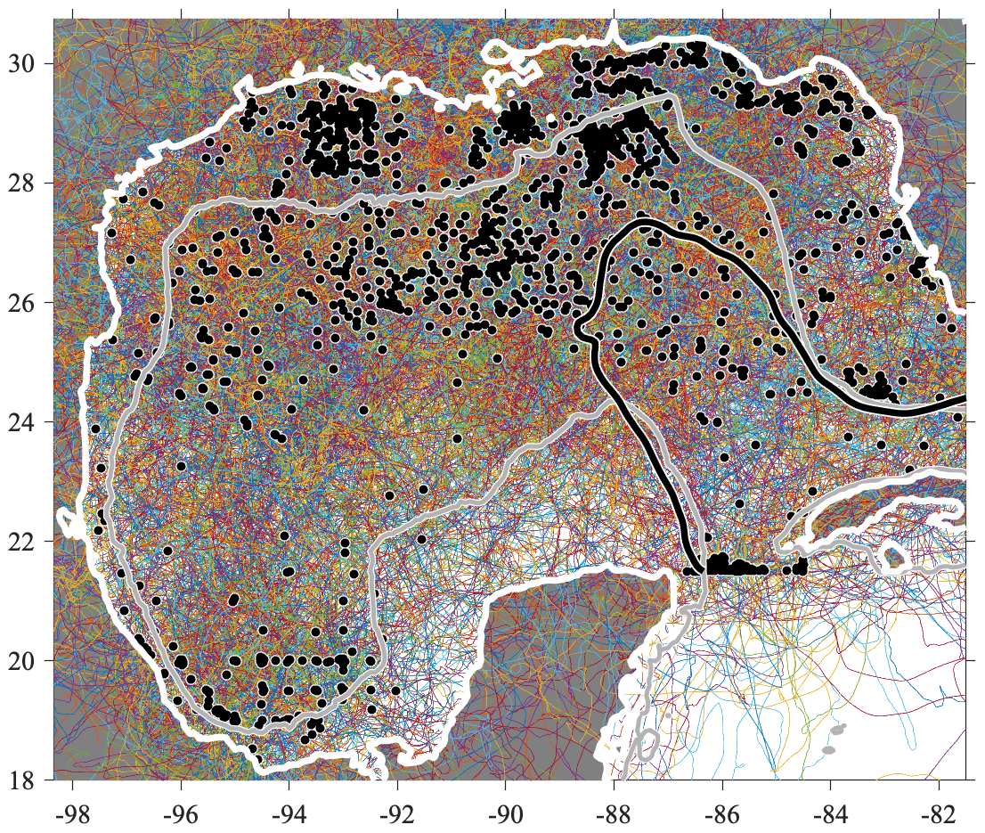
Figure 11As in Fig. 1 but for trajectories of a noise dataset the same size as the original dataset. As described in the text, the noise is constructed on a trajectory-by-trajectory basis to have matching first- and second-order statistics as well as a similar velocity spectrum, with the exception than the velocity spectrum is constrained to be isotropic. The heavy white contour is the coastline.
4.4 Physical properties of ridges and ridge averages
To the various ellipse quantities introduced in Sect. 2, we will add several more that are particularly relevant for the study of eddies. Firstly we note that just as the displacement signal of a modulated oscillation in two dimensions describes an ellipse, so too does the associated velocity signal. Following Lilly and Gascard (2006), once the ellipse parameters are known for a displacement signal x⋆(t), the parameters of the ellipse on the velocity plane associated with can be found at once; see Appendix E therein. The semi-axes of the velocity ellipse will be denoted and . Then
are respectively the instantaneous geometric mean radius of the ellipse and a measure of the ellipse velocity. Here V(t), which is a signed analogue of κ for the velocity ellipse, is called the kinetic energy velocity since V2(t) gives the kinetic energy associated with the modulated elliptical motion.
The quantities V(t), b(t), ξ(t), and ω*(t) can all be of either sign. The former three are positive for counterclockwise motion and negative for clockwise motion, whereas ω*(t) is positive for cyclonic motion and negative for anticyclonic motion. This distinction is not important for our Northern Hemisphere study, but this is relevant for a global application.
To compactly summarize the results of the ridge analysis, we will look at properties averaged along the duration of a ridge. Denote the time average of some quantity q(t) along a ridge by
where times ti and tf mark the start and end of the ridge. Then a set of aggregate quantities representing average properties along a ridge is
where care has been taken to form the average in an appropriate way for each quantity. Thus reflects the time-averaged area associated with the elliptical signal, gives its time-averaged kinetic energy, and and are temporal averages weighted by the instantaneous signal power . Note that , , and are all signed quantities, consistent with their instantaneous versions.
4.5 Ridge analysis initial results
The results of applying the ridge analysis using the settings described above to both the surface drifter dataset, and to the noise dataset, are summarized in Fig. 12 through scatterplots of ridge-averaged quantities. Here the x axis is the ridge-averaged geometric mean radius in all panels. The real-world data are shown at the left and the noise dataset in the center column; the right column, discussed later, presents an edited version of the real-world dataset. In the data, 14471 ridges are found with . It turns out that the vast majority of these are due to inertial oscillations, with only 2520 ridges having . The noise dataset has 2045 ridges, comparable to the number of noninertial ridges in the drifter dataset, and reflecting the problem of false positives.

Figure 12Scatterplots of ridge-averaged quantities for the drifter data (a, d, g), for a noise dataset of the same size (b, e, h), and for the drifter dataset after the application of the noninertial criterion together with a significance criterion described later in the text (c, f, i), specifically ρX<0.1 with . In (a)–(c), the location of each ridge in ridge-averaged radius versus ridge-averaged velocity is shown. The color and size both represent the ridge length L, defined to be the number of periods an oscillation executes along the ridge. In (d)–(f), the y axis is now the ridge-averaged nondimensional frequency , while in (g)–(i) it is the ridge-averaged circularity . Diagonal lines in the upper row, and horizontal lines in the central row, mark lines of constant as noted in the legend. As the ridges are found for , the magnitudes of ridge-averaged frequencies will generally be within that range. In the right-hand column, vertical lines at km and km denote apparent transitions between different regimes.
A number of important features in the real-world data are apparent in the left column of Fig. 12. First, there is a large concentration of long-duration ridges with nondimensional frequencies , due to inertial oscillations. Second, there is a major asymmetry between cyclonic and anticyclonic events, as is most apparent from Fig. 12d. From km all the way up until about km, large-amplitude, long-duration cyclonic events are observed that have no parallel on the anticyclonic side. At still larger radii, the asymmetry reverses, and there is a tendency for larger-amplitude, longer-duration anticyclonic events that do not occur on the cyclonic side; see Fig. 12a. As discussed later, these are the large eddies shed from the Loop Current (e.g., Elliott, 1982; Lipphardt et al., 2008; Hall and Leben, 2016).
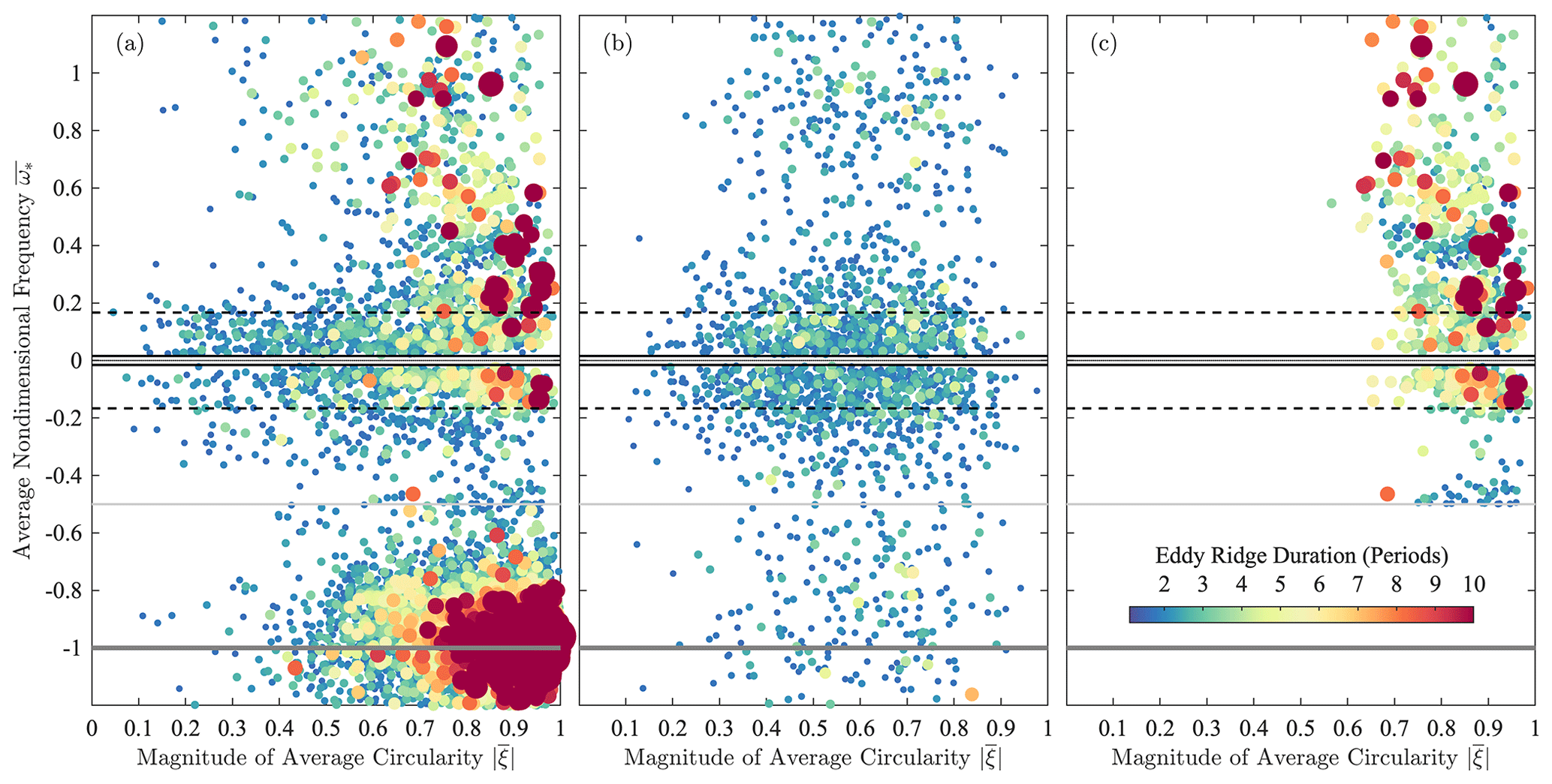
Figure 13As in the lower row of Fig. 12, with the nondimensional frequency on the y axis, but this time with the magnitude of the ridge-averaged circularity on the x axis. Again the real-world data (a) are on the left, the noise dataset (b) is in the center, and the real-world data after the application of the noninertial criterion and the significance criterion ρX<0.1 with are on the right (c).
Another presentation of the ridge-averaged properties is that in Fig. 13, in which the y axis is the nondimensional frequency , while the x axis is the magnitude of the circularity . These correspond, respectively, to the y axes in the second and third rows of Fig. 12. Here, the very high concentration of inertial oscillation ridges is apparent in the data in Fig. 13a; these are too stacked on top of each other in Fig. 12 to stand out. A gap occurs, in the frequency range between about and , where few events are seen. This gap, which does not occur on the cyclonic side, is most likely a manifestation of the stability boundary at , which as discussed previously affects only anticyclones. It is striking to see this dynamical feature emerge so readily from an analysis that treats all frequencies equally.
Inertial oscillations, as expected, are seen to be strongly circularly polarized in Fig. 13a. Outside of the inertial band, there is a tendency for longer-duration events to be more strongly circularly polarized than shorter-duration events. On the cyclonic side a transition occurs near . The longest-duration cyclonic events at higher frequencies, while still highly circularly polarized, have somewhat lower degrees of circularly polarization than the longest-duration cyclonic events at smaller frequencies. This is curious because one might expect high-frequency, highly nonlinear events to also be strongly circularly polarized.
The central columns of Figs. 12 and 13 show the properties of the ridges from the noise dataset presented earlier in Fig. 11. In comparison with the left columns, one sees that the real-world data contain ridges that have higher velocities, higher frequency magnitudes and thus higher degrees of nonlinearity, and stronger degrees of circular polarization than those occurring in the noise. In addition, ridge lengths L in the data are observed to be frequently much larger than in the noise. While there are 279 events in the data above the inertial band with lengths L>4, only six such events occur in a typical same-sized noise dataset. However, one also sees that a cloud of low-frequency, weakly circularly polarized events in the data aligns well with the noise distribution, suggesting that such events may not be statistically significant.
A final issue that should be mentioned is the possibility of contamination by the tides. The semidiurnal tide is excluded by our chosen frequency range, , except in the very northernmost part of the domain, as the M2 tidal frequency exceeds twice the local Coriolis frequency above about 28.7∘ N. Aliasing of semidiurnal tidal motions into eddy-like signals is therefore not expected to be a significant problem. The diurnal tide, meanwhile, is close to the inertial frequency over the range of latitudes spanned by the Gulf of Mexico and ranges from about 1.6f at 18∘ N to 1.0f at 30∘ N. Thus, the band where we might see diurnal tidal motions is to 1.6. A conspicuous tendency of oscillations at the diurnal frequency is not observed (not shown), and so tidal aliasing does not appear to be a major source of eddy-like variability. This topic could, however, be given more attention by examining the spectral signals of detected oscillations, which are far more narrowband for tidal signals than for eddies.
4.6 Assessing statistical significance
The plots from the previous section emphasize the importance of excluding false positives through an assessment of statistical significance. In doing so, it is desirable to avoid ad hoc cutoffs that involve the very properties we are most interested in studying, such as the radius, velocity, or Rossby number. If we consider what the essence of coherent vortices is, we can say that they are (i) long-lived features by definition and (ii) roughly circular, with the possibility of small degrees of eccentricity arising due to various dynamical processes such as ambient strain. This suggests that L and would be natural measures of significance that are agnostic to the primary physical properties of the vortex. The last two figures show that indeed the data and noise do have different distributions with respect to these two quantities.
A novel significance criterion is created as follows. Some to-be-determined quantity characterizing the ridges will be chosen as the basis for our significance test, denoted X and referred to as the significance parameter. Assume that the probability distribution of X is proportional to the function
which we will take to be a function of nondimensional ridge-averaged frequency, denoted ω in this section for convenience; here, we use “g” rather than the standard notation “f” because the latter symbol is already being used for the Coriolis frequency. Whereas probability distributions are defined to integrate to one, here we will make a different choice. The function gX(x;ω) is normalized such that, for a chosen nondimensional frequency bandwidth Δω, the integral
gives the ratio of the total number of ridge points within the band to the total number of data points, accounting for the possibility of multiplicities greater than unity. In other words, this integral gives the average number of ridge points per data point, or ridge density. Note that this is not quite the same as the probability of a data point being a ridge point, because a data point could be a member of more than one ridge. The dependence of gX(x;ω) on the choice of Δω is implicit.
The cumulative distribution function corresponding to gX(x;ω) is obtained by an integration to a particular x value,
Due to our choice of normalization, GX(x;ω) is the density of all ridge points in the band for which the significance parameter X takes on a value smaller than or equal to x. Integrating the density function in the opposite direction leads to a less familiar function
which is known as the complementary cumulative distribution function or, more colorfully, the survival function. 𝒮X(x;ω) gives the density of all ridge points in the frequency band for which the significance parameter X takes on a value greater than x.
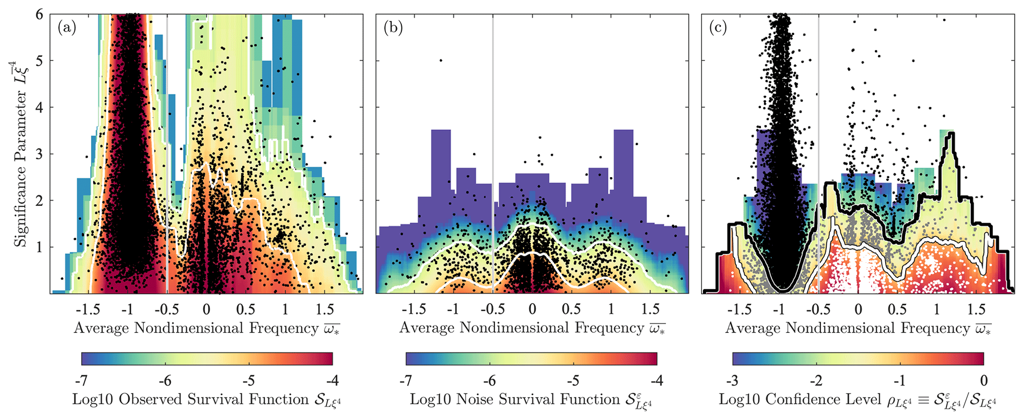
Figure 14A significance criterion for wavelet ridges in the Gulf of Mexico surface drifter dataset. The black dots in panel (a) show the locations of all ridges on the plane of the ridge-averaged nondimensional frequency versus , the product of ridge duration and fourth power of the ridge-averaged circularity. Bin-averaging in nondimensional frequency bins of width , and then cumulatively summing along the y axis from high values to low values, leads to an object called the complementary cumulative distribution function or survival function 𝒮X(x;ω) for , constructed here to be a function of frequency. The logarithm of the survival function is shown as the colored shading in (a), with white lines being the 10−5 and 10−6 contours. Panel (b) is the same as (a) but for the noise dataset. Since this dataset is 10 times the size of the observations, for display purposes only 10 % of the dots are shown, and the histogram is divided by a factor of 10, thus making panels (a) and (b) directly comparable. Finally the logarithm of the ratio is shown in (c). The heavy white line in this panel marks the contour such that only 1 out of 10 events above this curve is expected to be a false positive. Similarly, the black line is the contour, above which only 1 out of 100 events is expected to be a false positive. Dots in this panel are those of the data, the same as in (a). The black and gray dots mark observed ridges falling above the 0.01 and 0.1 contours, respectively. Those falling below the contour, shown as white dots, are judged to be statistically insignificant. The thin vertical gray line in all panels marks . Events to the left of this line likely represent inertial oscillations, apparent as the prominent peak in the vicinity of , rather than coherent eddies.
Comparing the estimated survival function of the data to that of the noise will allow us to assess whether an event's properties are extreme enough to warrant classifying it as statistically significant. We will choose , the product of the ridge length L and the fourth power of the ridge-averaged circularity , to be the significance parameter, for reasons to be discussed shortly. The construction of our measure of significance is described with reference to Fig. 14. In panel (a), a black dot is placed marking the joint location of and for each ridge in the data, and in panel (b) the same is done for a noise dataset of the same size as the original data. These dots are the sampled expressions of the density function of the data gX(x;ω) and also that of the noise, denoted .
The density functions gX(x;ω) and are then estimated by forming histograms of as a function of nondimensional frequency. These are formed in 1000 overlapping nondimensional frequency bands with the bandwidth set to , and with 2000 bins between zero and 20 for the values of . For better resolution of the noise histogram, it is computed using 10 different realizations, then divided by 10 to ensure that it reflects the average properties of a dataset of the same size as the original. Cumulatively summing these two histograms along the y axis, but from top to bottom instead of the more usual bottom to top leads to estimates of the survival functions and for the data and noise for the case . These are shown as the colored shading in Fig. 14a and b.
The ratio of the estimated survival function of the noise to that of the data
is a measure of statistical significance that will be called the density ratio, shown for in Fig. 14c. Consider the contour , the white line in this panel. Ridges with properties above this line occur in each frequency band only 10 % as often in the noise dataset as in the original data. Therefore, only 1 in 10 events in the data with properties above this line is expected to be a false positive under the null hypothesis of the isotropic velocity spectrum. Similarly, events above the black contour at occur only 1 % as often in the noise as in the data; thus only 1 in 100 is attributable to the null hypothesis.
The significance parameter X has been chosen as follows. Either L or is a natural choice, since ridges associated with eddies are distinguished from those arising from the noise by being generally longer in duration as well as exhibiting polarizations that are more consistently near-circular. However, the events judged as being significant using either X=L or are substantially non-overlapping, which suggests creating a parameter that combines information about both length and polarization. The ridge length weighted by a power of the circularity, , constitutes such a combined parameter. Varying α, we find that α=4 corresponds to a maximum in the number of total oscillations – that is, the sum of L over all ridges – judged to be significant at the ρ=0.1 level, indicating that this choice is efficiently combining information from L and . Thus, we choose here. However, because different choices of significance parameter may be appropriate for different situations, the distributed dataset includes ρ values for for α=0 through 6, as well as for .
In a previous version of this analysis, we used a significance criterion computed on the L vs. plane, grouping all events together regardless of frequency. However, simulations of noise with different spectral slopes showed that the generation of ridges due to noise is more efficient for white noise and less efficient for more strongly sloped processes. Consequently, our original frequency-independent criterion tended to exaggerate somewhat the significance of events at low frequencies, where the velocity spectra are generally flat, compared to higher frequencies where the spectra are sloped. The refined criterion developed here corrects this shortcoming while still including information from both L and .
In establishing a measure of statistical significance, we have refrained from using the language of statistical hypothesis testing, e.g., significance levels and p values. In statistical terminology, the probability under the null hypothesis of observing a value in a parameter that is more extreme than a given observation is known as the p value of that observation. The ρ value by contrast gives the estimated probability that a detected event is actually a false positive that has been incorrectly accepted; these are related but different. The ρ value could also be seen as being similar to the “false discovery rate” in multiple hypothesis testing introduced by Benjamini and Hochberg (1995). Because it seems natural to approach this problem in terms of the densities of detected events, our proposed measure of statistical significance differs from those commonly used in the hypothesis testing literature. Formally connecting these ideas would be a useful exercise but is outside the scope of the present paper.
4.7 Results
Excluding now those ridges having a density ratio below for (the white contour in Fig. 14c), as well as those with nondimensional frequencies below (the vertical gray line) in order to reject inertial oscillations, we obtain 1033 statistically significant ridges remaining, or about 41 % of the 2520 noninertial ridges. In the noise, by construction, there are only about 10 % as many ridges meeting these criteria in a typical dataset of the same size as the original data. The distribution of events from this statistically significant, noninertial ridge set, termed the eddy ridges, will be briefly described in this section.
Ridge-averaged properties of the eddy ridges are shown in the right column of Fig. 12. The major feature is the asymmetry between cyclones and anticyclones noted in the Introduction. Three regimes are apparent: km, dominated by long-lived, highly nonlinear cyclones, with only relatively weak and short-duration anticyclones; 10 km km, dominated by nonlinear and very long-lived cyclones with nondimensional frequencies often greater than one-sixth, again with only relatively brief anticyclones, and with a notable lack of anticyclones at strong negative frequencies below ; and , which is increasingly dominated by long-lived anticyclones as one moves to larger radii.
The ellipses corresponding to these eddy ridges are those shown in the earlier Fig. 2. The ellipse inversion equations, Eqs. (28)–(31), are applied to the extracted signals, and the resulting ellipses are plotted with a temporal spacing equal to the estimated period . The center of each ellipse, with latitude and longitude , is then estimated as the residual after subtracting the ridge from the full trajectory; see Eqs. (57) and (58). Ridges are colored by their nondimensional instantaneous frequency magnitude , which when multiplied by two gives an estimate of the magnitude of the Rossby number of the oscillatory flow.
Overall there is a striking difference in geographic distribution between cyclones and anticyclones. Cyclones are concentrated in the eastern, western, and southern Gulf of Mexico, generally excluding the shallow-shelf regions. The anticyclones are concentrated primarily over the Loop Current and due west of it, corresponding to the deepest part of the basin (see the bathymetry map in Fig. 1 of Lilly and Pérez-Brunius, 2021a), with a smaller number of events seen north or northwest of the Loop Current. The two patterns are observed to be generally complementary, with cyclonic events and anticyclonic events occurring in largely disjoint locations.
The distribution of anticyclonic events exhibits many large features with . Although not apparent in the map, one may observe trains of large ellipses tending to form near the Loop Current, then drifting westward, filling the central latitudes of the Gulf of Mexico. Such events are capturing the well-known Loop Current Eddies (e.g., Elliott, 1982; Lipphardt et al., 2008; Hall and Leben, 2016) that form periodically as pinch-off events from the Loop Current. From the right column of Fig. 12, especially in panel (c), one sees that there are many more anticyclones than cyclones for km, and especially for km. In this size class one also observes a number of long-lived, highly circular features on the anticyclonic side – the orange and red circles in Fig. 12 – but only a handful of similar features on the cyclonic side.
A cluster of cyclonic activity is seen in Fig. 2 to occur in the southwestern Gulf of Mexico, a region known as the Bay of Campeche. The observed ellipses there span a range of sizes, including a concentration in the large size class with km. This is consistent with the known presence of a quasi-permanent vortex, the Campeche Gyre, in that region (Padilla-Pilotze, 1990; Vázquez De La Cerda et al., 2005; Pérez-Brunius et al., 2013) and suggests that the eddy ellipses could be employed to usefully study its variability.
Two areas of energetic cyclonic eddy activity with roughly 10 to 50 km radius ellipses – the intermediate size class in the right-hand column of Fig. 12 – are the vicinity of the Loop Current and the western Gulf of Mexico. In both areas, one sees cyclonic ellipses with large nondimensional frequency magnitudes , hence large Rossby numbers, as well as long durations L; such events are almost entirely absent from the anticyclonic side of the distribution. These events correspond in the Fig. 2b to the yellow to orange colors, with many medium-sized ellipses occurring in long trains. In the east, these align with the periphery of the Loop Current and may be identified with the so-called Loop Current Frontal Eddies or LCFEs that form in the strong cyclonic shear zone on the current's flank (e.g., Le Hénaff et al., 2014). Cyclones with similar sizes and degrees of nonlinearity are observed in the west in Fig. 2b, with a notable absence at central longitudes. Whether this gap is a real feature or the result of a sampling issue is not immediately clear. Cyclones are known to occur in the western Gulf of Mexico, although most commonly in its northwest corner; see, e.g., Merrell and Morrison (1981) and Hamilton et al. (2002). The similarity with LCFEs suggests investigating the possibility of a similar origin for the western cyclones, either in the shear zone of the Loop Current or in those of the Loop Current Eddies.
Cyclone vs. anticyclone asymmetries at the mesoscale are expected on theoretical grounds (Matsuura and Yamagata, 1982; Cushman-Roisin and Tang, 1990; Arai and Yamagata, 1994; Cho and Polvani, 1996) and have also been reported in observations in studies that apply the spin parameter method to surface drifters (Griffa et al., 2008; Lumpkin, 2016). The details of this asymmetry would be expected to vary regionally. In our Gulf of Mexico eddy census, the occurrence of intense mesoscale cyclones that are much smaller than the anticyclones is perhaps not surprising, since at least some of the cyclones are believed to form from instabilities on the periphery of larger anticyclonic structures. Further investigation of the reasons behind the observed asymmetry, and the extent to which it generalizes to other parts of the ocean, would be a promising topic for future investigation.
Finally, the small-radius ( km), highly nonlinear cyclones seen in the right-hand column of Fig. 12 are visible as the small red circles distributed throughout the Gulf of Mexico. Far fewer events in this size class occur on the anticyclonic side. In particular, events with are populous on the cyclonic side but dynamically forbidden (and excluded from the census) on the anticyclonic side. While it is well known through remote sensing and sun-glint photographs that small cyclonic eddies are ubiquitous in the upper ocean (Munk et al., 2000; Eldevik and Dysthe, 2002), in situ observations of these so-called “spiral eddies” have proved elusive. See Lumpkin and Elipot (2010) for a rare example of a submesoscale vortex observed through surface drifters, their Fig. 6, due to “an exceptional and extremely anomalous case” of two drifters trapped in the same 10 km eddy. The results here, in which we can detect submesoscale features in individual trajectories, suggest that the fact that they are not more commonly seen in drifter trajectories is the result of a technical limitation in existing analysis methods, and not because they are not present or not resolved.
This paper has presented a method for extracting the displacement signals associated with coherent eddies, and for estimating the properties of the features that generated those signals, from large Lagrangian datasets. The method is rooted in ideas taken from the signal analysis literature, such as the analytic signal, modulated oscillations, and wavelet analysis. As these ideas are not yet all widely known in oceanography, they were introduced in some detail and discussed in the context of the eddy-detection problem.
A modification of an existing analysis method, multivariate wavelet ridge analysis, to prohibit sign transitions between cyclonic and anticyclonic polarizations renders it more suitable for this application. The main innovation, however, is a means of determining statistical significance, which is done through the creation of a null hypothesis in the form of a noise dataset constructed to match the basic statistical properties of the real-world data, yet lacking organized oscillatory features arising from spectral peaks. A significance criterion is proposed in which the distribution of a combined parameter, reflecting both the number of oscillations executed as well as the degree of circular polarization, in the data is compared with that of the noise as a function of frequency, in order to identify parameter regimes in which the noise is unlikely to have generated the observed features.
The statistically significant features emerging from an application to a large surface drifter dataset from the Gulf of Mexico were briefly discussed. It is clear that there is much to be learned about the Gulf of Mexico eddy field through studying these eddy ellipses. Here, in order to maintain a focus on the analysis method, the attention paid to physical results is intentionally kept to a minimum. These will be thoroughly investigated in a follow-up paper.
The incorporation of a criterion for determining statistical significance makes possible the application of the eddy-extraction method to very large datasets. This has great potential not only for studying eddies in real-world data with a new level of detail, but also for providing a novel means of comparing eddy characteristics from numerical models with those from observations. In particular, the eddy census for the Gulf of Mexico indicates that large-scale studies of submesoscale cyclonic vortices from in situ data are now possible for the first time. The distribution of a self-contained analysis routine, discussed below, is aimed to help facilitate the usage of this method by other investigators.
It is intended that this paper provides the groundwork for a multi-paper effort to solve the eddy extraction and property estimation problem as completely and rigorously as possible. Future efforts will include (i) examining the behavior of the method with regard to exact analytic vortex solutions such as those reviewed in Lilly (2018); (ii) exploring the potential of ridge analysis in the light of the connections established by Lilly (2018) between Lagrangian ellipse properties and the kinematic flow properties of vorticity, strain, and divergence; (iii) understanding the bias estimate of Lilly and Olhede (2012a) in terms of eddy dynamics through applications to idealized numerical models as well as to analytic solutions; and finally (iv) connecting this Lagrangian trajectory perspective to the rigorous Lagrangian field theory of Haller and Beron-Vera (2012) and related works.
The synthetic signal shown in Fig. 4a is formed using the ellipse generation equation, Eq. (1), with parameters
where ωo=0.05 rad d−1, κo=10 km, and T=1000 d, the latter being the signal duration. The semi-axis lengths are recovered via Eqs. (32) and (33). These choices lead to a clockwise circulating ellipse with a linearly growing amplitude, κ(t), that increases 6-fold over the signal duration T and also a linearly increasing orbital frequency, , that doubles. The ellipse is purely circular for the first quarter of its duration, . After that, it begins to become increasingly elliptical, reaching a vanishing circularity ξ(t)=0 at t=T while steadily precessing in the clockwise direction at a rate that is 10 % of its initial orbital frequency, .
The time-varying period corresponding to this signal, shown in Fig. 8b as the thin gray line, is computed by differentiating the generating ellipse parameters as . This is based on the form of Eq. (36) for the instantaneous frequency in terms of the canonical ellipse parameters.
The composite signal shown in Fig. 5 is constructed by adding the elliptical signal generated above to (i) a uniform westward drift at 0.5 cm s−1 plus (ii) a stochastic component. For the latter, we use a Matérn velocity process, shown by Lilly et al. (2017) to be equivalent to damped fractional Brownian motion, as implemented by the jLab function maternoise. Referring to Eq. (47) in that reference, the velocity standard deviation σ is set to σ=0.25 cm s−1, the spectral slope parameter α is chosen as α=1 giving a high-frequency decay of ω−2, and the damping parameter λ is set to λ=0.1 d−1. This velocity process is then cumulatively summed to generate a displacement signal.
Table A1Some important symbols used in this paper, together with variables from the GOMED dataset. The quantities in the second and third sections of the table are all the variables appearing in GOMED.
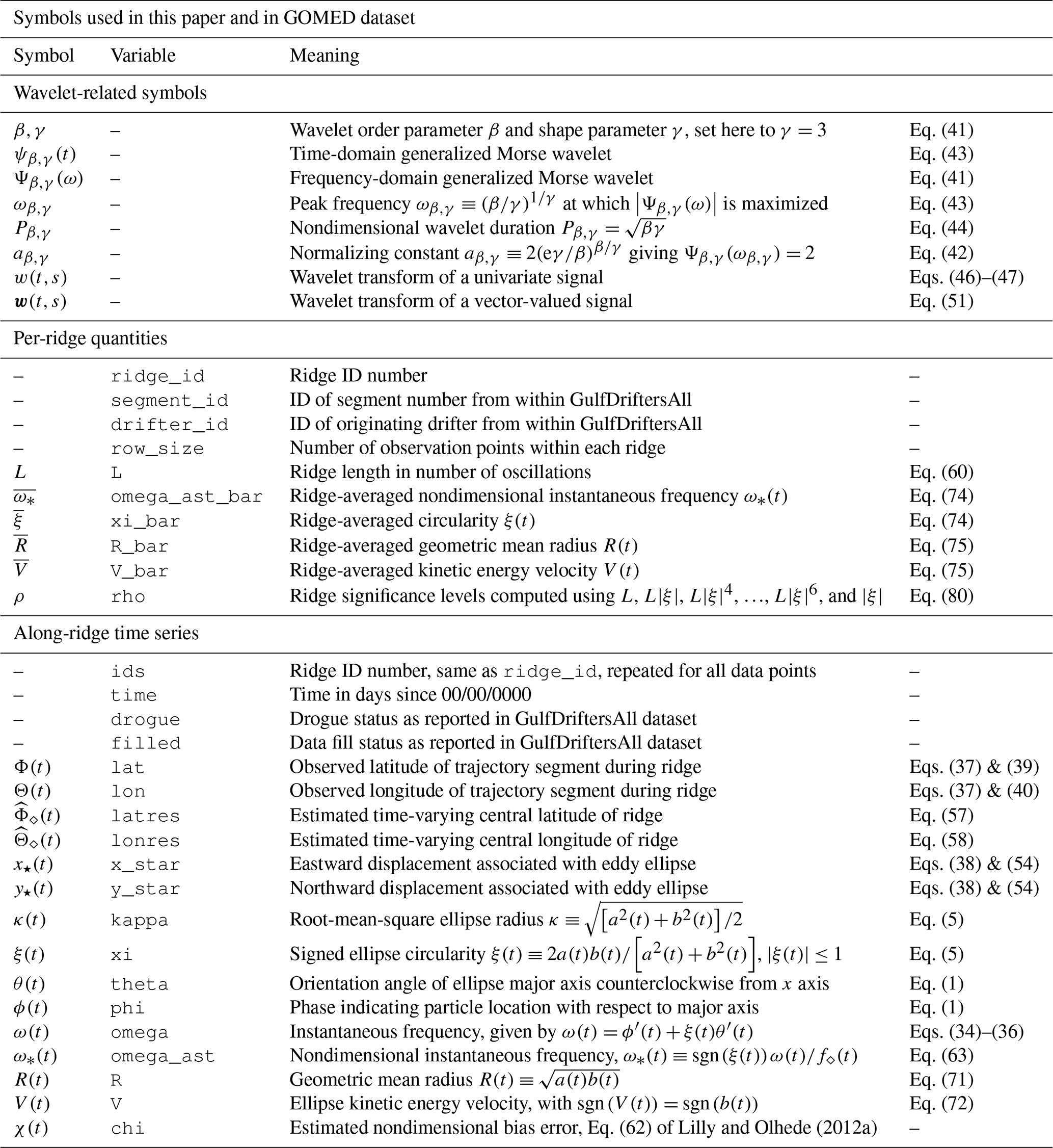
All numerical code required for the analysis carried out in this paper is distributed to the community as a part of jLab, the lead author's open-source data analysis toolbox for MATLAB, available at GitHub (https://github.com/jonathanlilly/jLab, last access: 16 March 2021) and Zenodo (https://doi.org/10.5281/zenodo.4547006, Lilly, 2021) and with extensive documentation found at http://www.jmlilly.net/doc/jLab.html (last access: 16 March 2021).
The centerpiece needed for this work is a new function, eddyridges, that implements the one-sided multivariate wavelet ridge analysis on an entire multi-instrument Lagrangian dataset. This may be applied either to latitude–longitude trajectories, as we have done here, or to trajectories on the x–y plane such as may be output from a numerical model. This function extends and greatly simplifies the approach used in Lilly and Gascard (2006) and Lilly et al. (2011), which involved directly calling the lower-level ridgewalk function implementing the ridge analysis. Construction of the noise dataset is done through the use of the function noisedrifters, and the significance levels are then assessed through eddylevels. Assorted other functions for computing ellipse properties, integration and differentiation on the sphere, and so forth are also included; see the jEllipses and jOceans modules. Finally, the toolbox contains scripts for creating the gomed.nc dataset, called make_gomed, and for generating all figures in this paper, called makefigs_gulfcensus.
Whereas for simplicity the handling of spherical geometry has been discussed herein using a small angle expansion about a fixed point, the numerical implementation in eddyridges takes a different approach that offers better performance for trajectories covering large distances on the surface of the Earth. This algorithm, using a routine called spheretrans, which works as follows. First, latitudes and longitudes are converted to a position in three-dimensional space, and the wavelet transform of that displacement signal in three dimensions is taken. The wavelet transform is then projected back onto a plane tangent to the Earth, centered on the time-varying center of the oscillation in each band of the transform considered separately. The multivariate ridge analysis is then applied to the resulting bivariate wavelet transform vector. Thus the method uses a projection about a moving point that is suitable for each oscillation considered separately, rather than a single fixed point for an entire dataset.
The dataset utilized in this paper is the consolidated surface drifter dataset created by Lilly and Pérez-Brunius (2021a) and referred to as GulfDriftersAll therein. While a subset of these data is proprietary and unfortunately cannot be redistributed, the bulk of that dataset is publicly available and is released to the community as the NetCDF file GulfDriftersOpen, available at https://doi.org/10.5281/zenodo.3985916 (Lilly and Pérez-Brunius, 2021b).
The results of applying the multivariate wavelet ridge analysis to GulfDriftersAll are distributed to the community as the Gulf of Mexico Eddy Dataset (GOMED) at https://doi.org/10.5281/zenodo.3978803 (Lilly and Pérez-Brunius, 2021c). In keeping with conditions stipulated by the primary funding agent, this dataset is made freely available for academic use with the agreement that it shall not be sold, profited from, or redistributed. Table A1 provides an overview of all variables contained in GOMED, which is distributed as the NetCDF file gomed.nc. Variables include extracted eddy displacement signals for all ridges, significant or not, detected using the settings described herein, as well as the time-varying ellipse parameters and estimated ellipse center location. The data include eddy displacement signals for all ridges, as well as the time-varying ellipse parameters and estimated ellipse center locations. The instantaneous frequency is also included, as is the instantaneous bias estimate derived by Lilly and Olhede (2012a). The data are organized as appended trajectory data that can be readily separated through the use of the ids field, or by calling the jLab function ncload. The ridge length L and ridge-averaged circularity are also included, as is the measure of statistical significance ρ.
JML was responsible for the theory, coding, analysis, and writing. PPB was responsible for obtaining funding, for the planning, deployment, and upstream processing of several of the datasets utilized herein, for managing the sharing of the GOMED dataset, and for finding the legal pathway to make this dataset publicly available. She also provided regional expertise and guidance throughout this project.
The authors declare that they have no conflict of interest.
This is a contribution of the Gulf of Mexico Research Consortium (CIGoM). We acknowledge the specific request of Petróleos Mexicano (Pemex) to the Hydrocarbon Fund to address the environmental effects of oil spills in the Gulf of Mexico that made this project possible. We are grateful to Paula García, Argelia Ronquillo, Favio Medrano, and the support from Dirección de Telemática and Dirección de Impulso a la Innovaciń y el Desarrollo at CICESE, as well as Omar Monroy (Mink Global), for their help in the IT and legal aspects required for making GOMED available. Finally, we wish to thank the two anonymous reviewers for their constructive feedback.
This research has been partially funded by the Mexican National Council for Science and Technology – Mexican Ministry of Energy – Hydrocarbon Fund, project 201441. The work of Jonathan M. Lilly was supported in part by award no. 1658564 from the Physical Oceanography program of the United States National Science Foundation.
This paper was edited by Stefano Pierini and reviewed by two anonymous referees.
Alpers, W., Brandt, P., Lazar, A., Dagorne, D., Sow, B., Faye, S., Hansen, M. W., Rubino, A., Poulain, P.-M., and Brehmer, P.: A small-scale oceanic eddy off the coast of West Africa studied by multi-sensor satellite and surface drifter data, Remote Sens. Environ., 129, 132–143, https://doi.org/10.1016/j.rse.2012.10.032, 2013. a
Arai, M. and Yamagata, T.: Asymmetric evolution of eddies in rotating shallow water, Chaos, 4, 163–175, https://doi.org/10.1063/1.166001, 1994. a
Armi, L., Hebert, D., Oakey, N., Price, J. F., Richardson, P., and Rossby, H.: Two years in the life of a Mediterranean salt lens, J. Phys. Oceanogr., 19, 354–370, https://doi.org/10.1175/1520-0485(1989)019<0354:TYITLO>2.0.CO;2, 1989. a
Bedrosian, E.: A product theorem for Hilbert transforms, Proc. IRE, 51, 868–869, https://doi.org/10.1109/PROC.1963.2308, 1963. a
Benjamini, Y. and Hochberg, Y.: Controlling the false discovery rate: a practical and powerful approach to multiple testing, J. Roy. Stat. Soc. B Met., 57, 289–300, https://doi.org/10.1111/j.2517-6161.1995.tb02031.x, 1995. a
Bosse, A., Fer, I., Lilly, J. M., and Søiland, H.: Dynamical controls on the longevity of a non-linear vortex: the case of the Lofoten Basin Eddy, Sci. Rep.-UK, 9, 13448, https://doi.org/10.1038/s41598-019-49599-8, 13448, 2019. a
Bower, A. S., Hendry, R. M., Amrhein, D. E., and Lilly, J. M.: Direct observations of formation and propagation of subpolar eddies into the subtropical North Atlantic, Deep-Sea Res., 39, 15–41, https://doi.org/10.1016/j.dsr2.2012.07.029, 2013. a
Cetina-Heredia, P., Roughan, M., van Sebille, E., Keating, S., and Brassington, G. B.: Retention and leakage of water by mesoscale eddies in the East Australian Current system, J. Geophys. Res.-Oceans, 124, 2485–2500, https://doi.org/10.1029/2018JC014482, 2019. a
Cho, J. Y.-K. and Polvani, L. M.: The emergence of jets and vortices in freely-evolving, shallow-water turbulence on a sphere, Phys. Fluids, 8, 1531–1552, https://doi.org/10.1063/1.868929, 1996. a
Cushman-Roisin, B. and Tang, B.: Geostrophic turbulence and the emergence of eddies beyond the radius of deformation, J. Phys. Oceanogr., 20, 97–113, https://doi.org/10.1175/1520-0485(1990)020<0097:GTAEOE>2.0.CO;2, 1990. a
Cushman-Roisin, B., Heil, W., and Nof, D.: Oscillations and rotations of elliptical warm-core rings, J. Geophys. Res.-Oceans, 20, 11756–11764, https://doi.org/10.1029/JC090iC06p11756, 1985. a
D'Asaro, E. A., Walker, S., and Baker, E.: Structure of two hydrothermal megaplumes, J. Geophys. Res.-Oceans, 99, 20361–20373, https://doi.org/10.1029/94JC01846, 1994. a
Daubechies, I. and Paul, T.: Time-frequency localisation operators: a geometric phase space approach II – The use of dilations and translations, Inverse Probl., 4, 661–680, https://doi.org/10.1088/0266-5611/4/3/009, 1988. a
de Jong, M. F., Søiland, H., Bower, A. S., and Furey, H. H.: The subsurface circulation of the Iceland Sea observed with RAFOS floats, Deep-Sea Res. Pt. I, 141, 1–10, https://doi.org/10.1016/j.dsr.2018.07.008, 2018. a
Delprat, N., Escudié, B., Guillemain, P., Kronland-Martinet, R., Tchamitchian, P., and Torrésani, B.: Asymptotic wavelet and Gabor analysis: Extraction of instantaneous frequencies, IEEE T. Inform. Theory, 38, 644–665, https://doi.org/10.1109/18.119728, 1992. a, b, c
Dong, C., Liu, Y., Lumpkin, R., Lankhorst, M., Chen, D., McWilliams, J. C., and Guan, Y.: A scheme to identify loops from trajectories of oceanic surface drifters: an application in the Kuroshio extension region, J. Atmos. Ocean. Tech., 28, 1167–1176, https://doi.org/10.1175/JTECH-D-10-05028.1, 2011. a, b
Eldevik, T. and Dysthe, K. B.: Spiral eddies, J. Phys. Oceanogr., 32, 851–869, https://doi.org/10.1175/1520-0485(2002)032<0851:SE>2.0.CO;2, 2002. a
Elliott, B. A.: Anticyclonic rings in the Gulf of Mexico, J. Phys. Oceanogr., 12, 1292–1309, https://doi.org/10.1175/1520-0485(1982)012<1292:ARITGO>2.0.CO;2, 1982. a, b, c
Flament, P., Lumpkin, R., Tournadre, J., and Armi, L.: Vortex pairing in an unstable anticyclonic shear flow: discrete subharmonics of one pendulum day, J. Fluid Mech., 440, 401–409, https://doi.org/10.1017/S0022112001004955, 2001. a, b
Furey, H., Bower, A., Pérez-Brunius, P., Hamilton, P., and Leben, R.: Deep eddies in the Gulf of Mexico observed with floats, J. Phys. Oceanogr., 48, 2703–2719, https://doi.org/10.1175/JPO-D-17-0245.1, 2018. a
Gabor, D.: Theory of communication, Proc. IRE, 93, 429–457, https://doi.org/10.1049/ji-1.1947.0015, 1946. a, b, c
Garreau, P., Garnier, V., and Schaeffer, A.: Eddy resolving modelling of the Gulf of Lions and Catalan Sea, Ocean Dynam., 61, 991–1003, https://doi.org/10.1007/s10236-011-0399-2, 2011. a
Gonella, J.: A local study of inertial oscillations in the upper layer of the ocean, Deep-Sea Res., 18, 775–788, https://doi.org/10.1016/0011-7471(71)90045-3, 1971. a
Gonella, J.: A rotary-component method for analyzing meteorological and oceanographic vector time series, Deep-Sea Res., 19, 833–846, https://doi.org/10.1016/0011-7471(72)90002-2, 1972. a
Griffa, A., Lumpkin, R., and Veneziani, M.: Cyclonic and anticyclonic motion in the upper ocean, Geophys. Res. Lett., 35, L01608, https://doi.org/10.1029/2007GL032100, 2008. a, b
Hall, C. A. and Leben, R. R.: Observational evidence of seasonality in the timing of Loop Current eddy separation, Dynam. Atmos. Oceans, 76, 240–267, https://doi.org/10.1016/j.dynatmoce.2016.06.002, 2016. a, b, c
Haller, G.: An objective definition of a vortex, J. Fluid Mech., 525, 1–26, https://doi.org/10.1017/S0022112004002526, 2005. a
Haller, G. and Beron-Vera, F. J.: Geodesic theory of transport barriers in two-dimensional flows, Physica D, 241, 1680–1702, https://doi.org/10.1016/j.physd.2012.06.012, 2012. a
Hamilton, P., Berger, T. J., and Johnson, W.: On the structure and motions of cyclones in the northern Gulf of Mexico, J. Geophys. Res.-Oceans, 107, 3208, https://doi.org/10.1029/1999JC000270, 2002. a
Harvey, A. C.: Forecasting, structural time series models and the Kalman filter, Cambridge University Press, Cambridge, UK, https://doi.org/10.1017/CBO9781107049994, 1989. a
Huang, J. and Yang, L.: Vakman's analysis in L2(ℝ), Int. J. Comput. Math., 88, 545–554, https://doi.org/10.1080/00207161003631869, 2011. a
Inoue, R., Faure, V., and Kouketsu, S.: Float observations of an anticyclonic eddy off Hokkaido, J. Geophys. Res.-Oceans, 121, 6103–6120, https://doi.org/10.1002/2016JC011698, 2016. a
Kirwan Jr., A. D., Merrell Jr., W. J., Lewis, J. K., Whitaker, R. E., and Legeckis, R.: A model for the analysis of drifter data with an application to a warm core ring in the Gulf of Mexico, J. Geophys. Res.-Oceans, 89, 3425–3438, https://doi.org/10.1029/JC089iC03p03425, 1984. a, b
Kirwan Jr., A. D., Lewis, J. K., Indest, A. W., Reinersman, P., and Quintero, I.: Observed and simulated kinematic properties of Loop Current rings, J. Geophys. Res.-Oceans, 93, 1189–1198, https://doi.org/10.1029/JC093iC02p01189, 1988. a
Kloosterziel, R. C.: Viscous symmetric stability of circular flows, J. Fluid Mech., 652, 171–193, https://doi.org/10.1017/S0022112009994149, 2010. a
Kourafalou, V., Androulidakis, Y., Le Hénaff, M., and Kang, H.: The dynamics of Cuba Anticyclones (CubANs) and interaction with the Loop Current/Florida Current system, J. Geophys. Res.-Oceans, 122, 7897–7923, https://doi.org/10.1002/2017JC012928, 2017. a
Kunze, E.: Near-inertial wave propagation in geostrophic shear, J. Phys. Oceanogr., 15, 544–565, https://doi.org/10.1175/1520-0485(1985)015<0544:NIWPIG>2.0.CO;2, 1985. a
Lankhorst, M.: A self-contained identification scheme for eddies in drifter and float trajectories, J. Atmos. Ocean. Tech., 23, 1583–1592, https://doi.org/10.1175/JTECH1931.1, 2006. a
Le Hénaff, M., Kourafalou, V. H., Dussurget, R., and Lumpkin, R.: Cyclonic activity in the eastern Gulf of Mexico: Characterization from along-track altimetry and in situ drifter trajectories, Prog. Oceanogr., 120, 120–138, https://doi.org/10.1016/j.pocean.2013.08.002, 2014. a, b, c
Le Hénaff, M., Kourafalou, V. H., Androulidakis, Y., Smith, R. H., Kang, H., Hu, C., and Lamkin, J. T.: In situ measurements of circulation features influencing cross-shelf transport around northwest Cuba, J. Geophys. Res.-Oceans, 125, e2019JC015780, https://doi.org/10.1029/2019JC015780, 2020. a
Lilly, J. M.: Element analysis: a wavelet-based method for analyzing time-localized events in noisy time series, P. Roy. Soc. Lond. A Mat., 473, 20160776, https://doi.org/10.1098/rspa.2016.0776, 2017. a
Lilly, J. M.: Kinematics of a fluid ellipse in a linear flow, Fluids, 3, 16, https://doi.org/10.3390/fluids3010016, 2018. a, b, c, d, e, f
Lilly, J. M.: jLab: A data analysis package for Matlab v1.7.0, Zenodo, https://doi.org/10.5281/zenodo.4547006, 2021. a
Lilly, J. M. and Gascard, J.-C.: Wavelet ridge diagnosis of time-varying elliptical signals with application to an oceanic eddy, Nonlin. Processes Geophys., 13, 467–483, https://doi.org/10.5194/npg-13-467-2006, 2006. a, b, c, d, e, f, g, h, i, j, k, l
Lilly, J. M. and Olhede, S. C.: Wavelet ridge estimation of jointly modulated multivariate oscillations, in: 2009 Conference Record of the Forty-Third Asilomar Conference on Signals, Systems, and Computers, 1–4 November 2009, Pacific Grove, California, USA, 452–456, https://doi.org/10.1109/ACSSC.2009.5469858, 2009a. a, b, c
Lilly, J. M. and Olhede, S. C.: Higher-order properties of analytic wavelets, IEEE T. Signal Proces., 57, 146–160, https://doi.org/10.1109/TSP.2008.2007607, 2009b. a, b, c, d, e, f
Lilly, J. M. and Olhede, S. C.: On the analytic wavelet transform, IEEE T. Inform. Theory, 56, 4135–4156, https://doi.org/10.1109/TIT.2010.2050935, 2010a. a, b, c
Lilly, J. M. and Olhede, S. C.: Bivariate instantaneous frequency and bandwidth, IEEE T. Signal Proces., 58, 591–603, https://doi.org/10.1109/TSP.2009.2031729, 2010b. a, b, c, d, e, f, g, h, i
Lilly, J. M. and Olhede, S. C.: Analysis of modulated multivariate oscillations, IEEE T. Signal Proces., 60, 600–612, https://doi.org/10.1109/TSP.2011.2173681, 2012a. a, b, c, d, e, f, g, h, i, j
Lilly, J. M. and Olhede, S. C.: Generalized Morse wavelets as a superfamily of analytic wavelets, IEEE T. Signal Proces., 60, 6036–6041, https://doi.org/10.1109/TSP.2012.2210890, 2012b. a, b, c
Lilly, J. M. and Pérez-Brunius, P.: A gridded surface current product for the Gulf of Mexico from consolidated drifter measurements, Earth Syst. Sci. Data, 13, 645–669, https://doi.org/10.5194/essd-13-645-2021, 2021a. a, b, c, d, e
Lilly, J. M. and Pérez-Brunius, P.: GulfDrifters: a consolidated surface drifter dataset for the Gulf of Mexico (Version 1.1.0), Zenodo, https://doi.org/10.5281/zenodo.3985916, 2021b. a
Lilly, J. M. and Pérez-Brunius, P.: The Gulf of Mexico Eddy Dataset (GOMED), a census of statistically significant eddy-like events from all available surface drifter data (Version 1.1.0), Zenodo, https://doi.org/10.5281/zenodo.3978803, 2021c. a
Lilly, J. M., Scott, R. K., and Olhede, S. C.: Extracting waves and vortices from Lagrangian trajectories, Geophys. Res. Lett., 38, L23605, https://doi.org/10.1029/2011GL049727, 2011. a, b, c
Lilly, J. M., Sykulski, A. M., Early, J. J., and Olhede, S. C.: Fractional Brownian motion, the Matérn process, and stochastic modeling of turbulent dispersion, Nonlin. Processes Geophys., 24, 481–514, https://doi.org/10.5194/npg-24-481-2017, 2017. a, b
Lipphardt Jr., B. L., Poje, A. C., and Kirwan, A.: Death of three Loop Current rings, J. Mar. Res., 66, 25–60, https://doi.org/10.1357/002224008784815748, 2008. a, b, c
Lumpkin, R.: Global characteristics of coherent vortices from surface drifter trajectories, J. Geophys. Res.-Oceans, 121, 1306–1321, https://doi.org/10.1146/annurev-marine-010816-060641, 2016. a, b
Lumpkin, R. and Elipot, S.: Surface drifter pair spreading in the North Atlantic, J. Geophys. Res.-Oceans, 115, C12017, https://doi.org/10.1029/2010JC006338, 2010. a
Lumpkin, R. and Pazos, M.: Measuring surface currents with Surface Velocity Program drifters: the instrument, its data, and some recent results, in: Lagrangian Analysis and Prediction in Coastal and Ocean Processes, edited by: Griffa, A., Kirwan Jr., A. D., Mariano, A., Özgökmen, T., and Rossby, H., Cambridge University Press, Cambridge, UK, 39–67, https://doi.org/10.1017/CBO9780511535901.003, 2007. a
Mallat, S.: A wavelet tour of signal processing, edn. 2, Academic Press, New York, USA, https://doi.org/10.1016/B978-0-12-374370-1.X0001-8, 1999. a, b, c
Matsuura, T. and Yamagata, T.: On the evolution of nonlinear plantary eddies larger than the radius of deformation, J. Phys. Oceanogr., 12, 440–456, https://doi.org/10.1175/1520-0485(1982)012<0440:OTEONP>2.0.CO;2, 1982. a
McKiver, W. J. and Dritschel, D. G.: The stability of a quasi-geostrophic ellipsoidal vortex in a background shear flow, J. Fluid Mech., 560, 1–17, https://doi.org/10.1017/S0022112006000462, 2006. a
Meacham, S. P. and Flierl, G. R.: Vortices in shear, Dynam. Atmos. Oceans, 14, 333–386, https://doi.org/10.1016/0377-0265(89)90067-5, 1990. a
Merrell Jr., W. J. and Morrison, J. M.: On the circulation of the western Gulf of Mexico with observations from April 1978, J. Geophys. Res.-Oceans, 86, 4181–4185, https://doi.org/10.1029/JC086iC05p04181, 1981. a
Munk, W. H., Armi, L., Fischer, K., and Zachariasen, F.: Spirals on the sea, P. Roy. Soc. Lond. A Mat., 456, 1217–1280, https://doi.org/10.1098/rspa.2000.0560, 2000. a
Nerlove, M.: Distributed lags and unobserved components in economic time series, in: Ten Economic Studies in the Tradition of Irving Fisher, John Wiley & Sons Inc., New York, USA, 127–169, 1967. a
Olhede, S. C. and Walden, A. T.: Generalized Morse wavelets, IEEE T. Signal Proces., 50, 2661–2670, https://doi.org/10.1109/TSP.2002.804066, 2002. a
Padilla-Pilotze, A. R.: Evidence of a cyclonic eddy in the Bay of Campeche, Cienc. Mar., 16, 1–14, https://doi.org/10.7773/cm.v16i3.703, 1990. a, b
Papoulis, A.: The Fourier integral and its applications, McGraw-Hill Book Company Inc., New York, USA, 1962. a
Park, J., Lindberg, C. R., and Vernon III, F. L.: Multitaper spectral analysis of high-frequency seismograms, J. Geophys. Res.-Oceans, 92, 12675–12684, https://doi.org/10.1029/JB092iB12p12675, 1987. a
Percival, D. B. and Walden, A. T.: Spectral Analysis for Physical Applications, Cambridge University Press, New York, USA, https://doi.org/10.1017/CBO9780511622762, 1993. a
Pérez-Brunius, P., García-Carrillo, P., Dubranna, J., Sheinbaum, J., and Candela, J.: Direct observations of the upper layer circulation in the southern Gulf of Mexico, Deep-Sea Res., 85, 182–194, https://doi.org/10.1016/j.dsr2.2012.07.020, 2013. a, b
Picinbono, B.: On instantaneous amplitude and phase of signals, IEEE T. Signal Proces., 45, 552–560, https://doi.org/10.1109/78.558469, 1997. a, b, c
Ripa, P.: On the stability of elliptical vortex solutions of the shallow-water equations, J. Fluid Mech., 183, 343–363, https://doi.org/10.1017/S0022112087002660, 1987. a
Ruddick, B. R.: Anticyclonic lenses in large-scale strain and shear, J. Phys. Oceanogr., 17, 741–749, https://doi.org/10.1175/1520-0485(1987)017<0741:ALILSS>2.0.CO;2, 1987. a
Søiland, H. and Rossby, T.: On the structure of the Lofoten Basin Eddy, J. Geophys. Res.-Oceans, 118, 4201–4212, https://doi.org/10.1002/jgrc.20301, 2013. a
Testor, P. and Gascard, J.-C.: Large-scale spreading of deep waters in the western Mediterranean Sea by submesoscale coherent eddies, J. Phys. Oceanogr., 33, 75–87, https://doi.org/10.1175/1520-0485(2003)033<0075:LSSODW>2.0.CO;2, 2003. a
Thomson, D. J.: Spectrum estimation and harmonic analysis, P. IEEE, 70, 1055–1096, https://doi.org/10.1109/PROC.1982.12433, 1982. a
Trodahl, M., Isachsen, P. E., Lilly, J. M., Nilsson, J., and Kristensen, N. M.: The regeneration of the Lofoten Vortex through vertical alignment, J. Phys. Oceanogr., 50, 2689–2711, https://doi.org/10.1175/JPO-D-20-0029.1, 2020. a
Vakman, D.: On the analytic signal, the Teager-Kaiser energy algorithm, and other methods for defining amplitude and frequency, IEEE T. Signal Proces., 44, 791–797, https://doi.org/10.1109/78.492532, 1996. a, b, c
Vázquez De La Cerda, A. M., Reid, R. O., DiMarco, S. F., and Jochens, A. E.: Bay of Campeche circulation: an update, in: Circulation in the Gulf of Mexico: Observations and Models, edited by: Sturges, W. and Lugo-Fernández, A., no. 161 in Geophysical Monograph Series, American Geophysical Union, 279–293, https://doi.org/10.1029/GM161, 2005. a, b
Veneziani, M., Griffa, A., Garraffo, Z., and Chassignet, E.: Lagrangian spin parameter and coherent structures from trajectories released in a high-resolution ocean model, J. Mar. Res., 63, 753–788, https://doi.org/10.1357/0022240054663187, 2005a. a
Veneziani, M., Griffa, A., Reynolds, A. M., Garraffo, Z. D., and Chassignet, E. P.: Parameterizations of Lagrangian spin statistics and particle dispersion in the presence of coherent vortices, J. Mar. Res., 63, 1057–1083, https://doi.org/10.1357/002224005775247571, 2005b. a
Young, W. R.: Elliptical vortices in shallow water, J. Fluid Mech., 171, 101–119, https://doi.org/10.1017/S0022112086001386, 1986. a
The term “objective” is used here in its conventional sense of not being shaped by personal opinion, that is, non-subjective. This is not to be confused with its more technical definition, used by, e.g., Haller (2005), meaning invariant to variations of an observer's frame of reference.
The lead author thanks Shane Elipot for pointing out an error in earlier published versions of Fig. 3, in which the angle labeled φ here was incorrectly identified as ϕ.
The circularity is related to another measure of ellipse shape, the linearity used by Lilly and Gascard (2006) and Lilly and Olhede (2010b), defined as , where sgn(⋅) is the signum function defined in Eq. (17). The linearity and circularity are related through .
The complex conjugate that would normally appear on the wavelet's Fourier transform Ψβ,γ(sω) after applying the convolution theorem has been dropped because these particular wavelets are real-valued in the frequency domain.
The first author thanks Georgi Sutyrin for asking the question, with respect to this method, “What is the principle?”.
In the case of a univariate signal x(t), we have , and L can be interpreted in terms of the phase change along the ridge. For the multivariate case, the multivariate instantaneous frequency of Eq. (35) is no longer defined as the derivative of some phase, so it would appear this interpretation no longer holds.
Note that the match between the temporal mean velocities obtained by differencing the trajectories is approximate rather than exact, due to minor differences between differentiating trajectories and integrating velocities on the sphere in the numerical implementation used here.
- Abstract
- Introduction
- A model for particle motion in an eddy
- Ellipse extraction
- Application to the Gulf of Mexico drifter dataset
- Conclusions
- Appendix A: Construction of the synthetic signal
- Code availability
- Data availability
- Author contributions
- Competing interests
- Acknowledgements
- Financial support
- Review statement
- References