Effects of upwelling duration and phytoplankton growth regime on dissolved-oxygen levels in an idealized Iberian Peninsula upwelling system

We apply a coupled modelling system composed of a state-of-the-art hydrodynamical model and a low-complexity biogeochemical model to an idealized Iberian Peninsula upwelling system to identify the main drivers of dissolved-oxygen variability and to study its response to changes in the duration of the upwelling season and in the phytoplankton growth regime. We find that the export of oxygenated waters by upwelling front turbulence is a major sink for nearshore dissolved oxygen. In our simulations of summer upwelling, when the phytoplankton population is generally dominated by diatoms whose growth is boosted by nutrient input, net primary production and air–sea exchange compensate dissolved-oxygen depletion by offshore export over the shelf. A shorter upwelling duration causes a relaxation of upwelling winds and a decrease in offshore export, resulting in a slight increase of net dissolved-oxygen enrichment in the coastal region as compared to longer upwelling durations. When phytoplankton is dominated by groups less sensitive to nutrient inputs, growth rates decrease, and the coastal region becomes net heterotrophic. Together with the physical sink, this lowers the net oxygenation rate of coastal waters, which remains positive only because of air–sea exchange. These findings help in disentangling the physical and biogeochemical controls of dissolved oxygen in upwelling systems and, together with projections of increased duration of upwelling seasons and phytoplankton community changes, suggest that the Iberian coastal upwelling region may become more vulnerable to hypoxia and deoxygenation.

1 Introduction

Declining dissolved-oxygen (DO) levels in the world's oceans, including in the coastal realm, impact all marine life (Laffoley and Baxter, 2019), from microbes to higher trophic levels (Breitburg et al., 2018), with consequences ranging from ecological adaptations and shifts (Gilly et al., 2013) and changes of biogeochemical activity (Wright et al., 2012) to mass mortality events (Diaz and Rosenberg, 2008) and biodiversity restructuring (Vaquer-Sunyer and Duarte, 2008).

Coastal waters are generally eutrophic and characterized by substantial planktonic productivity at the surface which favours oxygen consumption through the remineralization of sinking organic matter, leading to low levels of DO in subsurface and near-bottom waters. Highly productive surface waters are typical of coastal upwelling regions and sustain socioeconomically important ecosystems. Upwelling systems are thus especially sensitive to episodic and long-term changes in DO levels with deleterious effects on marine life and human activities such as fisheries (Grantham et al., 2004; Hales et al., 2006; Paulmier and Ruiz-Pino, 2009; McClatchie et al., 2010; Roegner et al., 2011).

The western Iberian Peninsula Upwelling System (IPUS) is the northern branch of the Canary Upwelling System where the intra-annual variability of alongshore winds produces a seasonal upwelling–downwelling cycle (Wooster et al., 1976). In the summer and early fall, the Azores High migrates northward, causing a poleward alongshore wind that forces offshore Ekman transport of surface waters and the upwelling of subsurface waters, while downwelling prevails the rest of the year. Long-term studies of the seasonal upwelling in the IPUS have pointed to a weakening of upwelling winds over multi-decadal timescales (Sousa et al., 2017), but simulations of future climate indicate an enhancement of the upwelling due to the poleward migration of the Azores High and a lengthening of the upwelling season (Miranda et al., 2013; Rykaczewski et al., 2015; Sousa et al., 2017).

During the upwelling season, hydrographic and biogeochemical variability is primarily determined by the wind forcing that controls the inflow of offshore subsurface water masses onto the shelf (Álvarez-Salgado et al., 1993). DO levels in these subsurface waters are thought to diminish during the upwelling season due to the strong remineralization of sinking organic matter as well as to mixing with poorly ventilated waters of subtropical origins (Castro et al., 2006). Overall, DO appears to partly control the remineralization of dissolved organic carbon in the IPUS and more generally in key water masses of the North Atlantic (Álvarez-Salgado et al., 2013).

DO, in addition to being transported by the Ekman upwelling circulation, is also affected by the turbulent component of the circulation, characterized by (sub-)mesoscale fronts, filaments and eddies (Bettencourt et al., 2015; Capet et al., 2008; Chaigneau et al., 2009; Marchesiello et al., 2003; Montes et al., 2014; Vergara et al., 2016). These structures have a strong influence on the cross-shore transport and on the vertical redistribution of biogeochemical tracers (Bettencourt et al., 2017; Combes et al., 2013; Gruber et al., 2011; Hernández-Carrasco et al., 2014; Nagai et al., 2015; Renault et al., 2016; Rossi et al., 2013). In the Iberian basin, the Eastern North Atlantic Central Water (ENACW) mass of subtropical origin, whose archetypal concentrations of DO are initially low, would be ventilated by eddy-induced mixing with more oxygenated ENACW of subpolar origin (Pèrez et al., 2001).

From the biological perspective, the planktonic community structure can also affect DO in the water column, as this results from the balance between oxygen production by photo-autotrophs and respiration by both autotrophs and heterotrophs. Changes in the community composition should lead to changes in the DO budget of the continental shelf. In the Iberian upwelling, planktonic blooms tend to be dominated by large cells (micro-phytoplankton), such as diatoms (Moncoiffé et al., 2000; Rossi et al., 2013), which have lower respiration-to-photosynthesis ratios than dinoflagellates or cyanobacteria (López-Sandoval et al., 2014). Moreover, diatoms growth is thought to be positively correlated with the upwelling-driven nitrate inputs (Sarthou et al., 2005); in contrast, the growth of other planktonic groups can be insensitive to and even limited by newly upwelled nitrates (Mahaffey, 2005), especially when colimitation prevails or in the absence of necessary micro-nutrients. Thus, changes in the relative dominance of functional groups in the community can lead to different autotrophy–heterotrophy regimes and total DO levels.

In this paper, we perform a process-oriented study coupling an idealized IPUS configuration of a hydrodynamic model with a low-complexity biogeochemical model centred on oxygen. We focus on the mechanisms of DO change to assess the relative role and importance of physical (upwelling duration) and biogeochemical (functional planktonic community) processes in setting DO levels and distribution. Previous studies have focused on the seasonal and climatological modelling of the planktonic ecosystems and of dissolved oxygen (Marta-Almeida et al., 2012; Reboreda et al., 2014, 2015). Here, the spatiotemporal scales studied are shorter, since we are interested in the variations and forcing mechanisms of DO levels in response to successive and short-lived upwelling pulses, commonly observed in the IPUS during the upwelling season. The coupled physical–biogeochemical model is presented in Sect. 2; our results are shown and analysed in Sect. 3. We then discuss our findings and conclude in Sect. 4.

2 Materials and methods

2.1 The coupled model

The idealized IPUS is contained in a meridionally oriented stretch of continental shelf with constant bathymetry and limited zonally by the coast and the open ocean (Fig. 1). The domain has 300 km of length and width, with a shelf width of 50 km, which is characteristic of the Iberian shelf at 41^∘ N. The resolution of the spatial grid is 500 m, allowing for the simulation of summer upwelling seasons up to 90 d duration, with the associated upwelling front dynamics – mesoscale and submesoscale vortices and filaments – within acceptable computing time limits.

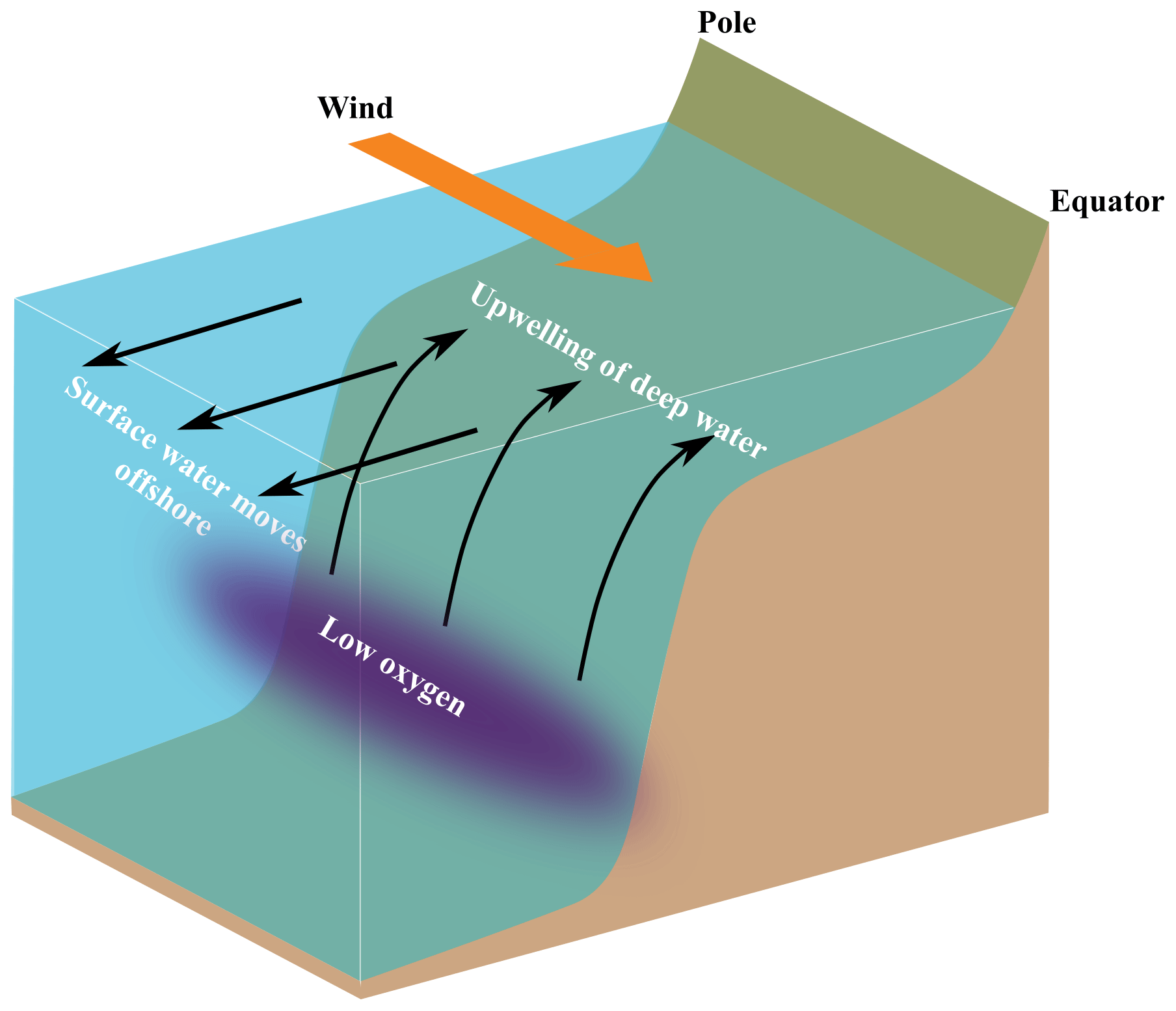
Figure 1 Idealized coastal upwelling configuration. The domain is periodic in the meridional (pole–Equator) direction.

The physical–biogeochemical model couples the 3D Regional Ocean Modelling System (ROMS; Shchepetkin, 2015; Shchepetkin and McWilliams, 2005), in its Coastal and Regional Ocean Community (CROCO) version (Debreu et al., 2012), to the low-complexity oxygen–phytoplankton–zooplankton biogeochemical model of Petrovskii et al. (2017) and Sekerci and Petrovskii (2015), hereafter SP2015. Oxygen is used as the main model currency, since it is central for the functioning of marine ecosystems (Breitburg et al., 1997, 2018). Oxygen is also at the heart of the photosynthesis and carbon fixation metabolic pathways for prokaryotic and eukaryotic algae, being a major electron acceptor (Mackey et al., 2008; Zehr and Kudela, 2009) and is needed for many biogeochemical reactions, including those involved in remineralization, which constantly occurs in the oceanic water column. The low-complexity O₂PZ model was directly implemented into the CROCO model following one of the already-embedded biogeochemical modules; it allows for maintaining the full capabilities and versatility of this community code while gaining in computing efficiency (allowing for extensive sensitivity studies and the consideration of submesoscale dynamics in oxygen cycling) as compared to the more complex biogeochemical modules already available within CROCO.

ROMS–CROCO is a hydrostatic primitive equation model, formulated in finite differences with time splitting in the barotropic (fast) mode and the baroclinic (slow) mode. It uses a terrain following vertical discretization in σ coordinates with 40 vertical levels. The prognostic variables are the horizontal barotropic and baroclinic momentum components, temperature and salinity. Free-surface displacement and vertical momentum are diagnostic variables. The horizontal advection of momentum and tracers is calculated from a third-order upstream-biased scheme. Horizontal mixing is Laplacian, along iso–σ surfaces, with diffusivity coefficients of 2 and 0.2 m² s⁻¹ for momentum and tracers, respectively. Vertical mixing uses the K-profile parameterization (KPP) scheme of Large et al. (1994). The model is initialized from rest; the initial temperature and salinity distributions are uniform in the horizontal, and the vertical profiles are taken from the World Ocean Atlas 2013 climatology (Boyer et al., 2013). Initial fields of the biogeochemical tracers (O₂, P and Z) are also horizontally homogeneous, and their vertical profiles are obtained from a water column (e.g. 1D) model version of the O₂PZ model (not shown). The channel is periodic in the meridional boundaries; the eastern boundary (coast) is modelled as a free-slip wall, and the western one (open ocean) is open with radiative boundary conditions for momentum and tracers. Within the westernmost 50 km, a sponge layer is applied with an increased horizontal viscosity of 200 m² s⁻¹ and a nudging timescale of 3 d in order to nudge all prognostic variables to their initial values over the offshore region. The bottom stress formulation is logarithmic with a roughness height of 0.01 m.

The model is forced by a cyclic uniform wind field. To promote the destabilization of the upwelling front, we introduce a small spatial perturbation to the wind field, whose amplitude is less than 1 % of the total wind speed and which has characteristic wavelengths of 10 and 50 km in the alongshore and cross-shore directions, respectively.

In the coupled model, the time evolution of DO, P and Z concentrations are given by, respectively,

$$\begin{array}{}\text{(1)}& {\displaystyle }\begin{array}{rl}\partial \left[{\mathrm{O}}_{\mathrm{2}}\right]/\partial t& +u\partial \left[{\mathrm{O}}_{\mathrm{2}}\right]/\partial x+v\partial \left[{\mathrm{O}}_{\mathrm{2}}\right]/\partial y+w\partial \left[{\mathrm{O}}_{\mathrm{2}}\right]/\partial z\\ & =k_{\mathrm{H}}\left({\partial }^{\mathrm{2}}\right[{\mathrm{O}}_{\mathrm{2}}]/\partial x^{\mathrm{2}}+{\partial }^{\mathrm{2}}[{\mathrm{O}}_{\mathrm{2}}]/\partial y^{\mathrm{2}})\\ & +\partial /\partial z(\langle [{\mathrm{O}}_{\mathrm{2}}{]}^{\prime }{w}^{\prime }\rangle -k_{\mathrm{V}}\partial \left[{\mathrm{O}}_{\mathrm{2}}\right]/\partial z)+V_{\mathrm{a}}(\left[{\mathrm{O}}_{\mathrm{2}}\right]\\ & -\left[{\mathrm{O}}_{\mathrm{2}}{]}_{\mathrm{sat}}\right)+AJ\left(z\right)f\left(\right[{\mathrm{O}}_{\mathrm{2}}\left]\right)\left[\mathrm{P}\right]-u_{\mathrm{r}}\left(\right[{\mathrm{O}}_{\mathrm{2}}],[\mathrm{P}\left]\right)\\ & -v_{\mathrm{r}}\left(\right[{\mathrm{O}}_{\mathrm{2}}],[\mathrm{Z}\left]\right)-m\left[{\mathrm{O}}_{\mathrm{2}}\right],\end{array}\text{(2)}& {\displaystyle }\begin{array}{rl}\partial \left[\mathrm{P}\right]/\partial t& +u\partial \left[\mathrm{P}\right]/\partial x+v\partial \left[\mathrm{P}\right]/\partial y+w\partial \left[\mathrm{P}\right]/\partial z\\ & =k_{\mathrm{H}}\left({\partial }^{\mathrm{2}}\right[\mathrm{P}]/\partial x^{\mathrm{2}}+{\partial }^{\mathrm{2}}[\mathrm{P}]/\partial y^{\mathrm{2}})+\partial /\partial z(\langle [\mathrm{P}{]}^{\prime }{w}^{\prime }\rangle \\ & -k_{\mathrm{V}}\partial \left[\mathrm{P}\right]/\partial z)+l(N\left)g\right(\left[{\mathrm{O}}_{\mathrm{2}}\right],\left[\mathrm{P}\right])\\ & -e\left(\right[\mathrm{P}],[\mathrm{Z}\left]\right)-\mathit{\sigma }\left[\mathrm{P}\right],\end{array}\text{(3)}& {\displaystyle }\begin{array}{rl}\partial \left[\mathrm{Z}\right]/\partial t& +u\partial \left[\mathrm{Z}\right]/\partial x+v\partial \left[\mathrm{Z}\right]/\partial y+w\partial \left[\mathrm{Z}\right]/\partial z\\ & =k_{\mathrm{H}}\left({\partial }^{\mathrm{2}}\right[\mathrm{Z}]/\partial x^{\mathrm{2}}+{\partial }^{\mathrm{2}}[\mathrm{Z}]/\partial y{)}^{\mathrm{2}})+\partial /\partial z(\langle [\mathrm{Z}{]}^{\prime }{w}^{\prime }\rangle \\ & -k_{\mathrm{V}}\partial \left[\mathrm{Z}\right]/\partial z)+\mathit{\kappa }(\left[{\mathrm{O}}_{\mathrm{2}}\right]\left)e\right(\left[\mathrm{P}\right],\left[\mathrm{Z}\right])-\mathit{\mu }[\mathrm{Z}],\end{array}\end{array}$$

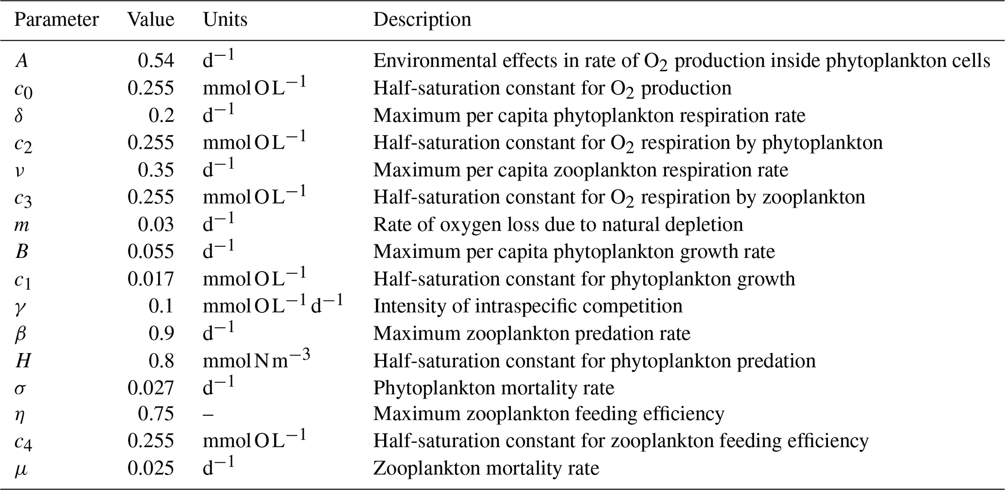
where $(u,v,w)$ is the 3D velocity field, k_H and k_V are the horizontal and vertical tracer diffusivities, and 〈…〉 are the vertical turbulent fluxes. The biogeochemical model O₂PZ (SP2015) defines the source terms of DO, P and Z in the coupled model. It simulates seven biogeochemical reactions between the three compartments (Fig. 2) as follows: in the DO equation (Eq. 1), the term AJ(z)f([O₂]) is the rate of O₂ production by photosynthesis and is modelled by a Monod parametrization $f\left(\right[{\mathrm{O}}_{\mathrm{2}}\left]\right)=c_{\mathrm{0}}/\left(\right[{\mathrm{O}}_{\mathrm{2}}]+c_{\mathrm{0}})$, where c₀ is a half-saturation constant. The term $J\left(z\right)=\mathrm{1}-\exp \left(\mathit{\alpha }\text{PAR}\right(z)/A)$ represents the light dependency of photosynthesis, with α=30 and the photosynthetically available radiation $\text{PAR}\left(z\right)=\text{PAR}\left(\mathrm{0}\right)\exp (-k_{w}z)$, with PAR(0)=355.19 W m⁻² and k_w=0.04 m⁻¹.

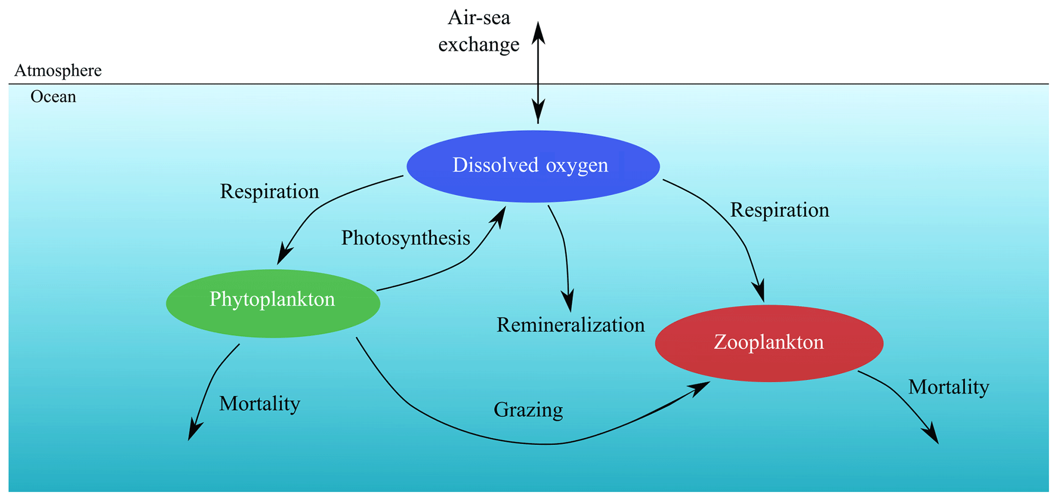
Figure 2 The oxygen–phytoplankton–zooplankton model of SP2015, adapted to the oceanic environment.

We distinguish here the terms “photosynthesis” from “carbon fixation” (Behrenfeld et al., 2008). Indeed, photosynthesis is the production of ATP (adenosine triphosphate) and NADPH (reduced form of NADP+; nicotinamide adenine dinucleotide phosphate) by the photosynthetic-electron-transport (PET) chain, and these two products are referred to as “photosynthate”. By contrast, carbon fixation refers to the use of photosynthate by the Calvin cycle to produce simple organic carbon products independently of light. SP2015 chose to highlight these two stages in their model formulation by decoupling carbon fixation from photosynthesis. The respiration by phytoplankton u_r is given by $u_{\mathrm{r}}\left(\right[{\mathrm{O}}_{\mathrm{2}}],[\mathrm{P}\left]\right)=\mathit{\delta }\left[{\mathrm{O}}_{\mathrm{2}}\right]\left[\mathrm{P}\right]/\left(\right[{\mathrm{O}}_{\mathrm{2}}]+c_{\mathrm{2}})$, where δ is the maximum per capita phytoplankton respiration rate and c₂ is the half saturation constant. Zooplankton respiration is similar: $v_{\mathrm{r}}\left(\right[{\mathrm{O}}_{\mathrm{2}}],[\mathrm{Z}\left]\right)=\mathit{\nu }\left[{\mathrm{O}}_{\mathrm{2}}\right]\left[\mathrm{Z}\right]/\left(\right[{\mathrm{O}}_{\mathrm{2}}]+c_{\mathrm{3}})$. The constants ν and c₃ have the same functions as δ and c₂ in u_r. A Monod function is a logical formulation to have respiration depending on oxygen concentration, since if the fluid environment becomes anoxic, then plankton cannot breathe so that respiration terms u_r and v_r vanish. The fourth term parametrizes bacterial respiration (oxygen loss due to natural depletion, e.g. remineralization). On top of the oxygen that is produced and consumed within marine ecosystems, a considerable part of dissolved oxygen eventually becomes gaseous and is then exchanged at the ocean–atmosphere interface, contributing to the estimations that more than one half of atmospheric oxygen is produced in the ocean (Harris, 1986). The remaining term of Eq. (2) is the air–sea flux of O₂, which is the product of the gas transfer velocity V_a, which depends on the square of the wind speed and on the Schmidt number (Wanninkhof, 1992), with the difference of the oceanic DO concentration and the solubility of O₂ in seawater.

In Eq. (2), phytoplankton growth g([O₂],[P]) is given by a linear growth term α([O₂])[P] minus intraspecific competition γ[P]², where γ is the intraspecific competition intensity. The per capita growth rate is a Monod function $\mathit{\alpha }\left(\right[{\mathrm{O}}_{\mathrm{2}}\left]\right)=B\left[{\mathrm{O}}_{\mathrm{2}}\right]/\left(\right[{\mathrm{O}}_{\mathrm{2}}]+c_{\mathrm{1}})$, where B is the maximum per capita growth rate in the large [O₂] limit and c₁ is the half saturation constant. The l(N) term is a Monod function $l\left(N\right)=k_{\mathrm{1}}N\left(\mathit{\rho }\right)/(k_{\mathrm{2}}+N(\mathit{\rho }\left)\right)$, where N(ρ) is a parametrization of nutrient availability based on the nitrate–density (ρ) relationships measured during an oceanographic cruise which surveyed the IPUS during upwelling season (the 2007 MOUTON – MOdélisation d’Un Théatre d’Opérations Navales – campaign; see also Rossi et al., 2010, 2013). This term is included here to circumvent the absence of nutrient limitation in the original O₂PZ model of SP2015. We chose to add a parametrization instead of a new equation for the nutrients because this last option would necessarily increase the complexity of the model.

SP2015 used a formulation where high oxygen increases phytoplankton growth but limits oxygen production by photosynthesis. The Warburg effect (Turner and Brittain, 1962) corresponds to the decrease of the photosynthesis rate at high oxygen concentrations so that the choice of f([O₂]) where high [O₂] limits [O₂] production makes sense. Moreover oxygen stimulates photorespiration which reduces photosynthesis yield. As soon as a water molecule (H₂O) undergoes photolysis in the chloroplast of oxygenic photosynthetic organisms, O₂ and ATP (adenosine triphosphate) are produced through both photosystems I and II. The products of photosynthesis (ATP) then enter the Calvin cycle to convert carbon dioxide and other compounds into glucose, which is the food that autotrophs need to grow. As such, we can relate the growth term α([O₂]) to [O₂] with a Monod function so that high [O₂] corresponds to a high growth rate. The predation term is $e\left(\right[\mathrm{P}],[\mathrm{Z}\left]\right)=\mathit{\beta }\left[\mathrm{P}\right]\left[\mathrm{Z}\right]/\left(\right[\mathrm{P}]+h)$, where β is the maximum predation rate and h is the half saturation constant. Phytoplankton mortality is σ[P]. Regarding zooplankton (Eq. 3), its feeding efficiency is a function of oxygen concentration $\mathit{\kappa }\left(\right[{\mathrm{O}}_{\mathrm{2}}\left]\right)=\mathit{\eta }[{\mathrm{O}}_{\mathrm{2}}{]}^{\mathrm{2}}/([{\mathrm{O}}_{\mathrm{2}}{]}^{\mathrm{2}}+c_{\mathrm{4}}^{\mathrm{2}})$, where η is the maximum feeding efficiency and c₄ is the half-saturation constant. Zooplankton mortality is given by μ[Z].

The parameters of the O₂PZ model were adjusted so that its 0D version (without advection or diffusion; see Table A3) has a steady state at values representative of the IPUS (see Appendix A).

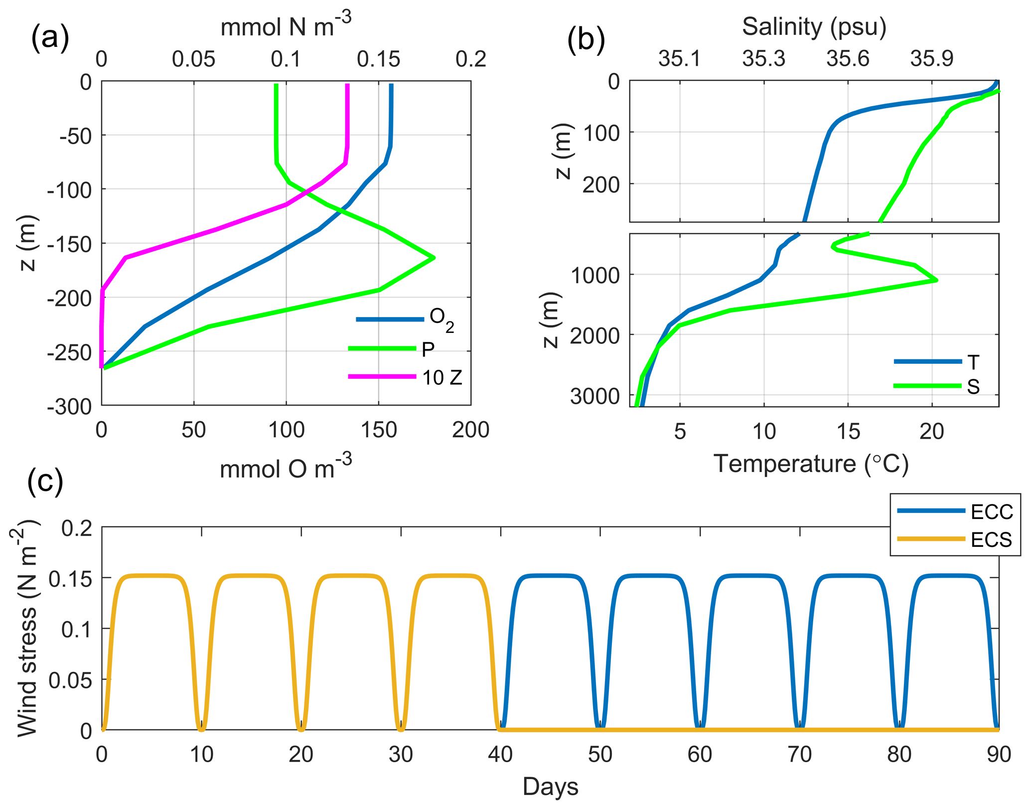
Figure 3 Initial conditions and wind forcing. (a) Initial profiles of O₂, P and Z. (b) Initial profiles of temperature (T) and salinity (S; in practical salinity units – psu). (c) Wind forcing regimes. ECC: nine wind cycles. ECS: four wind cycles.

2.2 Simulations

The coupled model is initialized at rest. Biogeochemical tracers are initialized from vertical profiles (Fig. 3a) obtained by a water column 1D model of the O₂PZ model that was run for a time long enough to reach stable vertical distributions (not shown). Using these profiles instead of climatological initial conditions allows for reducing the drift of the 3D coupled model (not shown). The initial temperature and salinity profiles (Fig. 3b) were taken from the World Ocean Atlas 2013 (WOA13; Boyer et al., 2013) data at 12^∘ W and 41^∘ N.

Table 1 Simulations. ECC is the reference simulation. All simulations are run for 90 d.

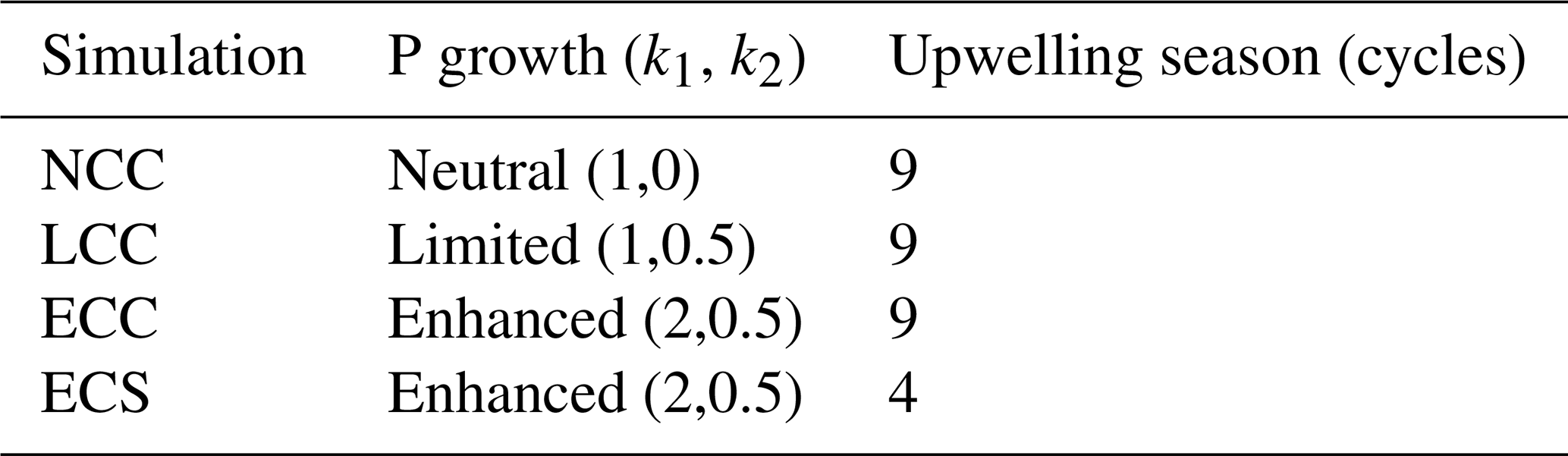
Our set of simulations (Table 1) is designed to investigate the sensitivity of the coastal DO inventory to upwelling duration and community structure (diatom dominated or not). We choose the duration of upwelling-favourable wind instead of its magnitude as a control factor because it has been shown to be a better predictor of coastal hypoxia (Feng et al., 2012; Forrest et al., 2011; Zhang et al., 2018). Community structure is set through the growth regime of the primary producers (phytoplankton) with respect to nutrient input. Thus, a diatom-dominated regime is simulated using enhanced growth rates due to nutrient input, for the (E)nhanced runs, while a non-diatom-dominated regime is simulated with growth rates (N)eutral to and (L)imited by nutrient input. We test the sensitivity of our coupled system to the relative dominance of diatoms in the community, as they have been suggested to decline over the long term, being gradually replaced by dinoflagellates and cyanobacteria (Gregg et al., 2017).

The effects of upwelling season length are studied by running two simulations with four and nine upwelling favourable wind cycles, maintaining a total simulation time of 90 d and considering a diatom-dominated phytoplankton community. The alongshore wind profiles (Fig. 3c) are based on the cyclic wind pulses that are characteristic of the summer–early-fall upwelling favourable conditions in the IPUS, especially those observed during the MOUTON campaign: 10 d pulses with a maximum wind speed of 12 m s⁻¹ (Rossi et al., 2013; Torres et al., 2003). The cross-shore wind component is zero in all cases. Despite the fact that “true” wind patterns observed over western Iberia are undoubtedly more variable (both in terms of direction and magnitude) than our idealized forcing inspired from a specific campaign, it provides the quickest development of a clear upwelling front generating small-scale instabilities. Note that sensitivity tests were performed (not shown) and revealed that the model responses are qualitatively similar among different wind strengths, given that the magnitude is high enough to ensure the development of the unstable upwelling front.

In situ observations of the IPUS, collected during the MOUTON 2007 campaign (Rossi et al., 2010, 2013) and compiled within the WOA13 (Boyer et al., 2013), are used not only to initialize but also to perform a comparison with the outputs of our simulations. The ECC simulation used the wind forcing and phytoplankton growth regimes that most resemble the IPUS region and therefore was chosen as the reference simulation.

Figure 4 Comparison of the ECC simulation with in situ observations. (a) Measured density vs. [O₂]. (b) Measured density vs. [Chl a] (fluorescence as a proxy for Chl a). (c) Modelled density vs. [O₂]. (d) Modelled density vs. [Chl a].

We compared the full ranges of densities ρ, DO concentrations [O₂] and chlorophyll a concentrations [Chl a] of the reference simulation to all compiled measurements collected during the MOUTON campaign. Given the low complexity of the biogeochemical model and the highly idealized physical setting, a fully quantitative comparison is out of the scope of this paper; however we confirm that the coupled model reproduces qualitatively well the ρ–[O₂] and ρ–[Chl a] relationships obtained from in situ observations.

3 Results and discussion

3.1 Dissolved oxygen in the idealized IPUS

Our coupled model reproduces well the upwelling circulation and the typical biological responses. Indeed, the upwelling of nutrient-rich waters induced by the mean wind-driven circulation promotes the growth of phytoplankton, leading to increased oxygen production by photosynthesis and the subsequent enrichment of oxygen in shelf waters (x<80 km; Fig. 5a), as compared with the lower [O₂] found in offshore waters (x>80 km). It also shows a low-[O₂] cell (∼50 mmol m⁻³), at the subsurface over the outer shelf (centred at 40 km and 60 m depth) because of the upwelling of low-O₂ waters, consistent with the shelf low-[O₂] cell (<200 µmol kg⁻¹) measured during the MOUTON cruise (e.g. Rossi et al., 2013). In a qualitative sense our idealized model results are similar to more realistic model studies, such as Gutknecht et al. (2013), which modelled the Benguela upwelling region and found a low-[O₂] plume for the climatological month of December at the shelf edge, and to observational studies such as Hales et al. (2006), which for the Oregon coast, measured [O₂] of 70–110 mmol m⁻³ in upwelled water at the shelf break, about 200 mmol m⁻³ less than at the surface, which is the same range of the vertical gradient simulated here.

The dynamics of the ECC simulation (Appendix B), are consistent with those documented by Durski and Allen (2005). A mean Ekman upwelling transport is established, moving subsurface waters upwards near the coast. The eddy-induced circulation (Cerovečki et al., 2009; Plumb and Ferrari, 2005) has the opposite sense to the mean circulation and is the strongest in the 50-to-100 km offshore range (Fig. B1). The result of the eddy-induced onshore and downward circulation is mainly seen in the subduction of the oxygen-rich waters just offshore the shelf edge, as suggested by the spatial pattern of the eddy stream function (Fig. B1).

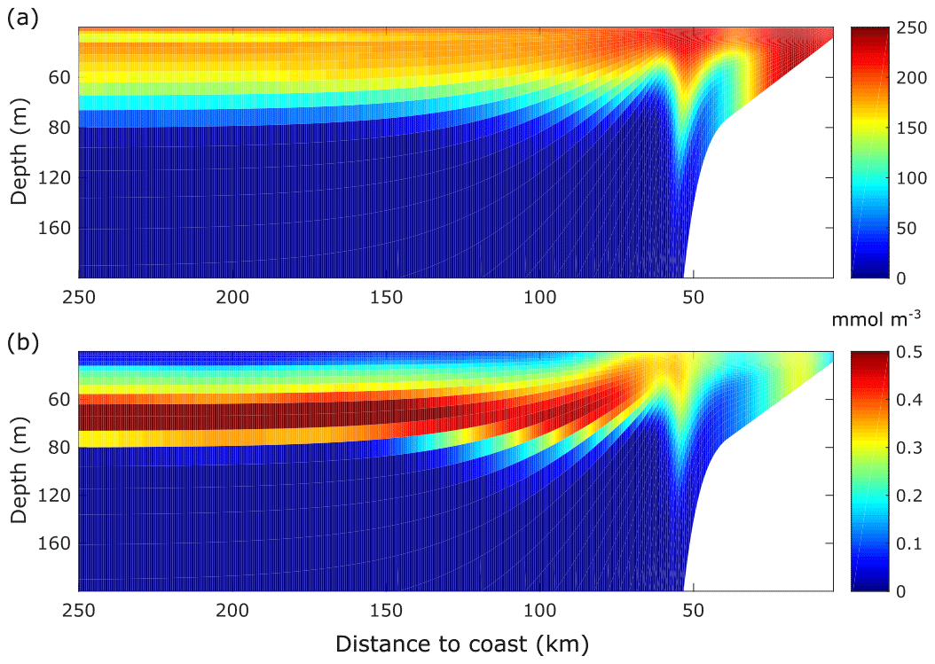
Figure 5 Mean [O₂] and [P] fields of the ECC simulation. (a) Time mean of the alongshore averaged [O₂] field. (b) Time mean of the alongshore averaged [P] field. Time means are computed from day 20 to day 90.

The spatial coincidence between the high-[O₂] and high-phytoplankton [P] concentration near the coast (Fig. 5) reflects O₂ enrichment caused by photosynthetic production (see Sect. 3.2 for a budget analysis). Since oxygen limits phytoplankton growth in our model, the low-[O₂] cell in the coast causes a matching low-[P] cell at the same location. Further offshore, subsurface [P] and [O₂] decrease as phytoplankton growth is limited by the lack of nutrients in the euphotic zone.

The subsurface [P] maximum between 60 and 80 m depth results from the trade-off between sufficient oxygen, light levels and nutrients availability. Consequently, the enhanced phytoplankton growth rate due to nutrients appears to compensate for the low oxygen levels, thus promoting phytoplankton growth. Moreover, the low [O₂] will maintain the zooplankton stocks at low levels, thus constraining the grazing pressure of zooplankton on phytoplankton.

The dominant length scales, i.e. the inverse of the wave number where the alongshore [O₂] anomaly field spectrum has a maximum, vary with time and the distance to the coast (Fig. 6a). After day 30, between 50 and 150 km offshore, we observe the emergence of dominant length scales of 150 km in an intermittent fashion, in a process that agrees with previous studies of the growth and decay of large mesoscale structures in coastal upwelling systems (Durski and Allen, 2005).

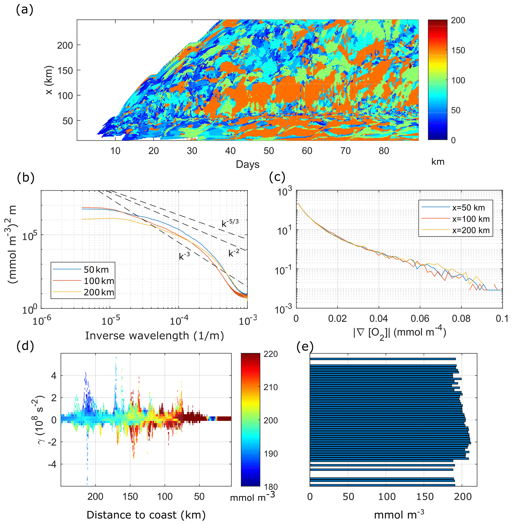
Figure 6 (a) Peak wavelength of the surface [O₂] alongshore wavenumber spectrum as a function of time and offshore shore distance. (b) Time mean surface [O₂] alongshore wavenumber spectrum at x=50, 100 and 200 km offshore. [O₂] spectra computed from anomalies with respect to the alongshore mean. (c) PDF of time mean surface [O₂] gradient norm at x=50, 100 and 200 km. (d) Instantaneous distribution of surface [O₂] by x and γ at day 65. (e) Distribution of x-averaged [O₂] by γ at day 65. Time mean taken from day 20 to day 90.

Slopes of time-averaged spectra of alongshore [O₂] anomalies at three offshore locations (Fig. 6b) show, however, that the submesoscale has also a marked effect on the [O₂] field. All spectra are shallower than the k⁻³ slope of geostrophic turbulence (Charney, 1971), implying that the submesoscale is prominent in our simulations (Capet et al., 2008). The spectrum at x=50 km is the shallowest and the closest to the $k^{-\mathrm{5}/\mathrm{3}}$ slope in the range 8.10${}^{-\mathrm{4}}<k<{\mathrm{10}}^{-\mathrm{4}}$. In the lower k range ($k<{\mathrm{10}}^{-\mathrm{5}})$, the spectra at 50 and 100 km have higher energy than the spectrum at 200 km, as the dominant length-scale plot shows the largest dominant length-scales in the 50–150 km cross-shore region.

The probability density function (PDF) of the [O₂] gradient norm (Fig. 6c) has a heavy tail distribution, associated with intermittency (Capet et al., 2008; Castaing et al., 1990). The existence of long tails in all PDFs indicates that sharp [O₂] gradients are ubiquitous in the channel.

Turbulence redistributes oxygen through fronts and filaments (strain-dominated regions) as well as vortices (rotation-dominated regions). To analyse this process, we use the Okubo–Weiss criterion γ, which separates turbulent velocity fields in strain-dominated (γ>0) and rotation-dominated (γ<0) regions. More specifically, we compute the daily average surface [O₂] for each γ and binned shore distance x.

For day 65, the [O₂] distribution by (γ,x) (Fig. 6d) reproduces the cross-shore [O₂] gradient of coastal elevated [O₂] and lower offshore [O₂] (the background gradient; see also Fig. 5a), in the range γ∼0. Deviations from this background gradient are found along the cross-shore direction as we move to larger |γ|, implying that [O₂] anomalies with respect to the mean surface field are mainly found in filaments and vortices. Since the highest [O₂] levels are found in the shelf region, due to photosynthetic production, their presence further offshore strongly suggests offshore export by turbulent structures. We emphasize that offshore transport of [O₂]-rich water results in a net loss of O₂ for the continental shelf region.

The [O₂] anomalies found offshore in regions of positive and negative γ highlight the transport and dispersion of O₂ by (sub-)mesoscale structures from the shelf to the open ocean. We find that although the mean [O₂] as a function of γ (averaged over x in each γ bin) remains at ∼200 mmol m⁻³ (Fig. 6e), the [O₂] distribution is biased toward negative γ, as found by Combes et al. (2013) for tracers in the California current. Our results are also in line with those of Lovecchio et al. (2017) that demonstrate the importance of mesoscale processes for the zonal advection of tracers, with a key role of eddies, especially offshore the upwelling front.

The relative importance of the physical vs. the biological processes in controlling coastal oxygen dynamics was analysed in terms of the volume-averaged rate of change of DO due to physics (advection and mixing), biology (photosynthesis, community respiration and remineralization) and air–sea fluxes within a shelf control volume (from the coast to 50 km offshore and from the surface to 140 m depth) and averaged from day 20 to 90. The net enrichment rate, accounting for the physical and biological forcing, is positive (2.26 $\mathrm{mmol}{\mathrm{m}}^{-\mathrm{3}}{\mathrm{d}}^{-\mathrm{1}}$), and so, over time, the coastal oxygen inventory increases. DO concentrations are increased by biogeochemical processes at a rate of 4.27 $\mathrm{mmol}{\mathrm{m}}^{-\mathrm{3}}{\mathrm{d}}^{-\mathrm{1}}$ and by air–sea exchange (3.41 $\mathrm{mmol}{\mathrm{m}}^{-\mathrm{3}}{\mathrm{d}}^{-\mathrm{1}}$) but are limited by physical processes that remove O₂ from the coastal region (−5.42 $\mathrm{mmol}{\mathrm{m}}^{-\mathrm{3}}{\mathrm{d}}^{-\mathrm{1}}$) through lateral advection.

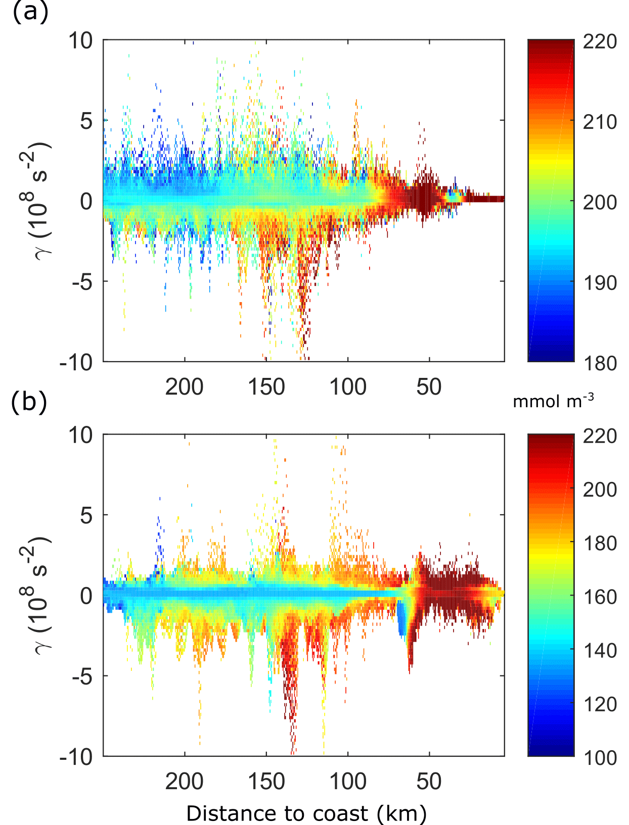
Figure 7 Time mean distribution of [O₂] by x and γ. (a) ECC. (b) ECS. Time mean taken from day 20 to 90.

3.2 Sensitivity of dissolved oxygen to upwelling duration and phytoplankton growth regimes

The reference simulation (ECC) has shown three major features: the appearance of subsurface low-[O₂] cells because of the upwelling of O₂-poor waters, the O₂ enrichment of surface levels, and the appearance of an [O₂] gradient between the biologically mediated enrichment at the inner shelf and the depleted offshore region. This gradient is, on the one hand, maintained by the upwelling circulation and, on the other hand, smoothed out by the cross-shore transport of O₂ by small-scale vortices and filaments. These effects are driven by the wind regime, which controls the upwelling dynamics and instabilities, and by the phytoplankton growth rate, which in turn affects phytoplankton concentrations. We now look at the sensitivity of the coupled model to these two drivers.

The continuous development of filaments and vortices in the ECC run maintains the offshore transport of dissolved oxygen (Fig. 7a). The wind shutdown in the ECS run causes a gradual decrease of turbulence which implies a diminution of the [O₂] redistribution by the cross-shore export physical processes, resulting in the creation of a sharper boundary between the oxygen-rich coastal waters and the depleted open ocean (offshore the upwelling front; Fig. 7b).

The phytoplankton growth regime impacts the mean [O₂] distribution, since nutrient neutrality (NCC) or limitation (LCC) results in the decrease of [O₂], when compared with the ECC run. The largest difference between the NCC and the ECC simulations (Fig. 8a) is observed in the coastal region, with maximum deviations from the ECC run of up to 100 mmol m⁻³. Offshore the front, on the other hand, we find an increase of [O₂] with respect to the ECC run, with the difference reaching ∼50 mmol m⁻³ at x=250 km. This positive difference is due to the absence of nutrient limitation so that phytoplankton growth and oxygen production persist in the nutrient-depleted surface levels.

The difference between the LCC and ECC cases (Fig. 8b) is also the highest in the shelf region, slightly above 100 mmol m⁻³. Offshore the front (x>50 km), the difference reduces to less than 50 mmol m⁻³, above 80 m depth, vanishing below this depth. In both cases, there is a signature of the low-[O₂] upwelling over the slope and shelf edge and the eddy-induced subduction just offshore the front (x=50 km).

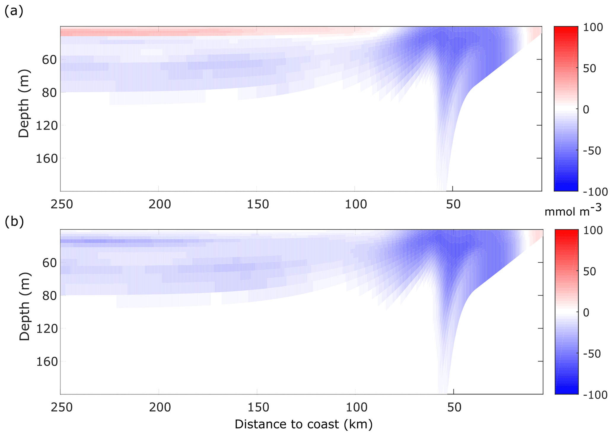
Figure 8 Difference in the time mean of dissolved oxygen with respect to the ECC run. (a) NCC. (b) LCC. Time mean taken from day 20 to 90.

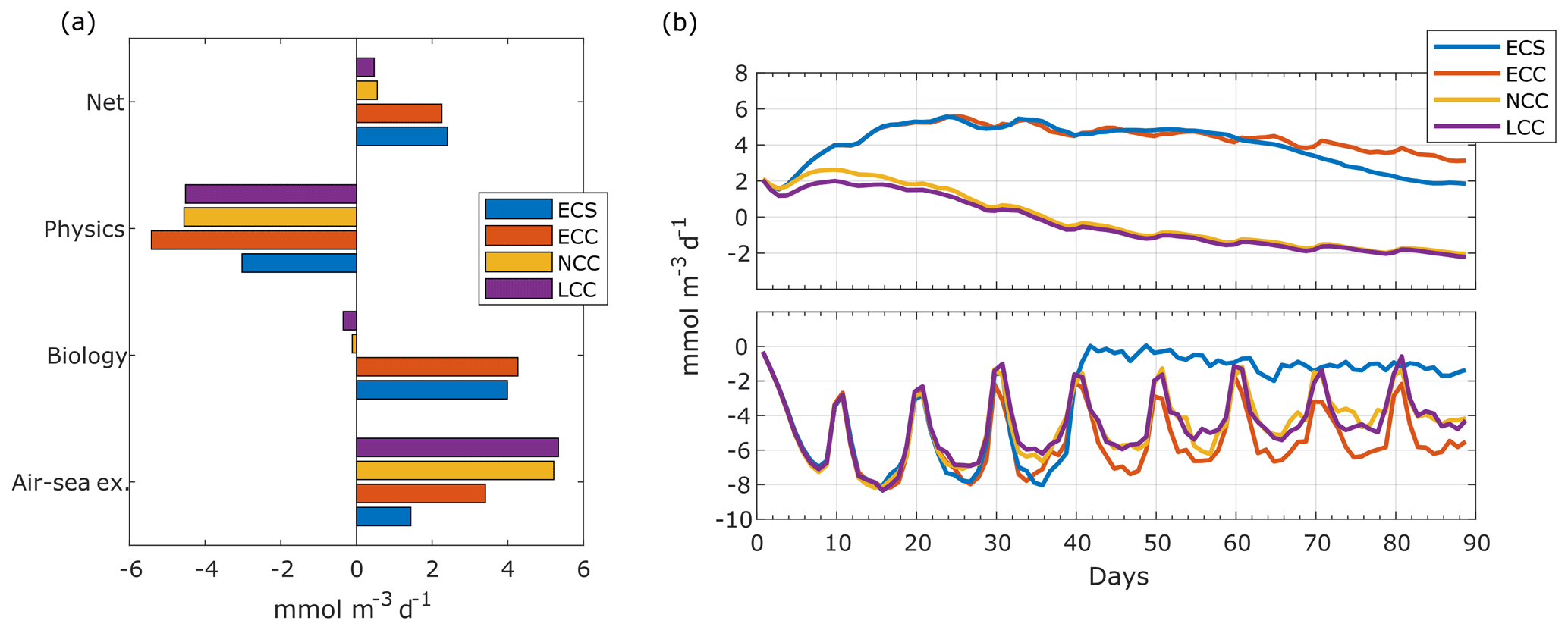
Figure 9 Dissolved-oxygen budgets in the coastal control volume. (a) Time mean rate of change of dissolved oxygen. Net value is the sum of physical, biological and air–sea exchange source and sink terms. Physical terms are the sum of cross-shore, alongshore and vertical advections as well as horizontal and vertical mixing. Biological term is oxygen photosynthetic production minus community respiration. Time mean taken from day 20 to 90. (b) Time series of average rate of change of dissolved oxygen in the coastal control volume due to biology (top) and physics (bottom).

When analysing O₂ budgets in the coastal control volume, from the shore to 50 km offshore and from the surface to 200 m of depth, the short upwelling duration simulation (ECS) results in a slight increase of the shelf [O₂] temporal-mean net rate of change by 6 % with respect to the ECC simulation (2.26 to 2.40 $\mathrm{mmol}{\mathrm{m}}^{-\mathrm{3}}{\mathrm{d}}^{-\mathrm{1}}$; Fig. 9a). Although every term in the oxygen mean budget for ECS is smaller than for ECC, the physical-sink decrease is slightly higher than the combined decrease in the biological source and sink ($Q_{{\mathrm{O}}_{\mathrm{2}}}$) and air–sea exchange.

The changes in the physical sink also occur faster than those in the biological terms. The wind cessation at day 40 causes an immediate decrease in the physical term (Fig. 9b, lower panel), while only after day 70 can we observe a significant difference between the biological source and sink terms of both the ECC and ECS simulations.

Changes in the phytoplankton growth regime modify the physical–biological balance of oxygen in the coastal control volume. The coastal region is net autotrophic ($Q_{{\mathrm{O}}_{\mathrm{2}}}>\mathrm{0}$) for ECC ($Q_{{\mathrm{O}}_{\mathrm{2}}}=\mathrm{4.27}$ $\mathrm{mmol}{\mathrm{m}}^{-\mathrm{3}}{\mathrm{d}}^{-\mathrm{1}}$) and ECS ($Q_{{\mathrm{O}}_{\mathrm{2}}}=\mathrm{3.99}$ $\mathrm{mmol}{\mathrm{m}}^{-\mathrm{3}}{\mathrm{d}}^{-\mathrm{1}}$) but becomes slightly net heterotrophic ($Q_{{\mathrm{O}}_{\mathrm{2}}}<\mathrm{0}$) when the phytoplankton growth becomes neutral to (NCC; $Q_{{\mathrm{O}}_{\mathrm{2}}}=-\mathrm{0.11}$ $\mathrm{mmol}{\mathrm{m}}^{-\mathrm{3}}{\mathrm{d}}^{-\mathrm{1}}$) or limited by (LCC; $Q_{{\mathrm{O}}_{\mathrm{2}}}=-\mathrm{0.35}$ $\mathrm{mmol}{\mathrm{m}}^{-\mathrm{3}}{\mathrm{d}}^{-\mathrm{1}}$) nutrients (Fig. 9a). This modifies the [O₂] gradients and the [O₂] lateral advective fluxes, and, as a result, the rate of oxygen loss through lateral advection decreases by about 15 % for NCC and LCC, with respect to ECC. The air–sea exchange of O₂ is also affected by the growth regime changes, as lower [O₂] will result in increased fluxes.

Overall, the phytoplankton growth regime has a stronger impact than the wind regime in the DO inventory in the shelf control volume. The NCC and LCC cases result in net rates of change of dissolved oxygen that are 75 %–80 % lower than in the reference case.

4 General discussion and conclusions

We built a coupled physical–biogeochemical model of an idealized seasonal coastal upwelling to study the effect of the upwelling season length and phytoplankton community structure on dissolved-oxygen inventory. The low-complexity O₂PZ model accounts for oxygen production by photosynthesis and consumption by both respiration and remineralization, but its simplicity does not allow for including other oceanographic processes that could influence oxygen cycling over shallow shelves, such as for instance the complex benthic-pelagic coupled processes (Capet et al., 2016). While we used data from the Iberian Peninsula upwelling to initialize and compare the range of values simulated by our model, our idealized configuration allows for drawing general conclusions about the mechanisms governing the dissolved-oxygen levels over the continental shelf. When compared to measurements, our model reproduces qualitatively the O₂–density relationship as well as the upwelling of oxygen-poor waters onto the shelf and the offshore transport of oxygen due to filaments and vortices. While the addition of air–sea exchange processes as well as our novel nutrient–density parametrization have probably contributed largely to simulate such realistic outputs despite the simple biogeochemical formulation, the coupled system could be further improved. One probably important task, which we keep for future studies, is to include realistic subsurface O₂ inputs from oceanic currents, as it has been shown to control largely O₂ dynamics over the shelf (Montes et al., 2014; Reboreda et al., 2015).

Although there is a clear separation of coastal waters with high [O₂] and offshore waters with low [O₂], the turbulent lateral transport of high-[O₂] water disrupts this picture, as oxygen-rich upwelling filaments and vortices are generated at the front and then travel offshore. This creates a sink of dissolved oxygen on the shelf that must be compensated by photosynthetic production and air–sea fluxes. In our reference simulation, with a repeated upwelling wind cycle, the net [O₂] rate of change was positive, owing to the predominance of the photosynthetic oxygen production and air–sea fluxes over the lateral transport of oxygen, which acts to remove it from the shelf region. Considering a shorter upwelling season (the ECS case with four 10 d upwelling wind cycles followed by wind cessation) reinforces somewhat the oxygen enrichment trend. When the phytoplankton community is dominated by groups that show nutrient limitation or neutral growth (LCC and NCC cases), the biological source weakens, and the shelf becomes net heterotrophic. The physical sink is also affected, producing a weaker loss of dissolved oxygen in the coastal upwelling. Air–sea exchange then maintains the (much lower) net oxygen enrichment trend.

Our findings that the oxygen inventory net rate of change is inversely proportional to the duration of the upwelling season is consistent with other studies (Adams et al., 2013; Siedlecki et al., 2015; Zhang et al., 2018). In the present, the IPUS is not hypoxic, but, as the upwelling season duration in the IPUS is thought to increase in the future (Miranda et al., 2013; Wang et al., 2015), it suggests an increased vulnerability of coastal regions to an episodic or long-term decrease of DO levels. The result of lower phytoplankton growth rates driving the shelf region from autotrophy to heterotrophy also points to an increased risk of loss of dissolved oxygen if trends for community shifts towards smaller or less-efficient phytoplankton (Gomes et al., 2014; Gregg et al., 2017; Head and Pepin, 2010; Zhai et al., 2013) are specifically confirmed for the IPUS. In permanent oxygen minimum zones (OMZs), changes in physical forcing (e.g. wind regime) and/or biological characteristics (e.g. size structure or functional types) can have dire implications for marine ecosystems and fishery management. Indeed, the measured expansion of the tropical Atlantic and Pacific OMZs (Stramma et al., 2008) implies a shallower upper boundary of the low-O₂ core and an increased sensitivity of oxygen levels over the continental shelf to upwelling winds, which are indeed predicted to intensify with climate change (Sydeman et al., 2014). Future work could be focused on understanding this high sensitivity and on anticipating how it would affect the stability of the coupled system in a changing climate.

Appendix A: Determination of O₂PZ model parameters

The biogeochemical component of the 3D coupled model (Eqs. 1–4) is a system of ordinary differential equations (ODEs) that computes the local time evolution of [O₂], [P] and [Z]. The ODE system accounts for the processes that move O₂, P and Z between different reservoirs. Each ODE of the model then expresses the input and output of the species from the specific reservoir. The dynamical properties of the ODEs will therefore influence the global behaviour of the coupled physical–biogeochemical model. When using coupled models such as Eq. (1), it is good practice to work in the vicinity of a known coexistence stable fixed point, i.e. a solution $X^{+}=\left(\right[{\mathrm{O}}_{\mathrm{2}}{]}^{+},[\mathrm{P}{]}^{+},[\mathrm{Z}{]}^{+}\ne (\mathrm{0},\mathrm{0},\mathrm{0})$ to Eqs. (2)–(4) that does not change with time and attracts nearby system trajectories. This guarantees that, when removing the advection and diffusion terms, the system will evolve to a constant state whose properties are already established (e.g. positive concentrations). The fixed points of the O₂PZ system are the states X⁺, where

$$\begin{array}{}\text{(A1)}& \mathrm{d}[{\mathrm{O}}_{\mathrm{2}}{]}^{+}/\mathrm{d}t=\mathrm{d}[\mathrm{P}{]}^{+}/\mathrm{d}t=\mathrm{d}[\mathrm{Z}{]}^{+}/\mathrm{d}t=\mathrm{0}.\end{array}$$

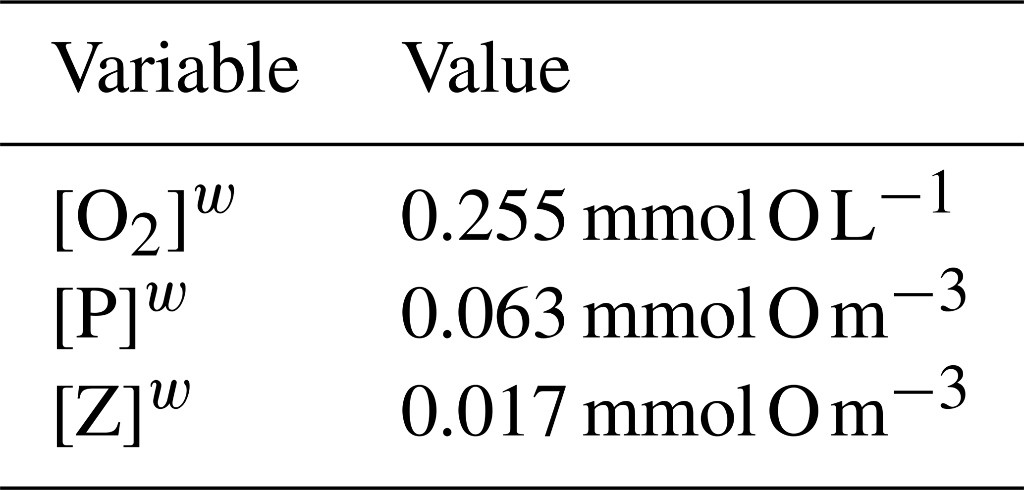
Since the system is nonlinear, a solution for Eq. (A1) is not straightforward, and approximate methods are then a good choice. Since the model will be used to study O₂ dynamics in coastal upwelling systems in the Iberian Peninsula western shelf and slope, it is logical that the model uses initial conditions that are characteristic of this region. The characteristic state $X^w=\left(\right[{\mathrm{O}}_{\mathrm{2}}{]}^w,{\left[\mathrm{P}\right]}^w,{\left[\mathrm{Z}\right]}^w)$ may be taken from a climatological dataset, in situ observations, remotely sensed data, etc. as long as it is representative of the actual values of ([O₂],[P],[Z]) in that region. Regarding the position of X^w in the state space, a simple proposition is that X^w is close to a coexistence steady state X⁰. This means that, if the model is initialized at X^w, it will converge to X⁰ and will not evolve to an extinction state or other steady states with unrealistic or uncharacteristic values of ([O₂],[P],[Z]) for the region. This is the approach adopted here to determine the values of the parameters of the system, and we adopt the characteristic values shown in Table A1 for the Iberian Peninsula upwelling.

The concentration of DO is taken from the climatological mean at 12^∘ W, 41^∘ N and 10 m depth. The phytoplankton concentration is obtained from ocean colour images of Chl a in the western Iberian shelf at approximately the same position of the DO reading, after converting it to nitrogen concentration using a ratio of 1.59 between Chl a and nitrogen content (Montes et al., 2014). Finally, the zooplankton concentration is found by using a phytoplankton-to-zooplankton ratio of 3.6, taken from SP2015 for the case of a stable coexistence state of the nondimensional model. For some parameters we adopt the values that are used elsewhere in the literature. To find the most adequate values of the remaining parameters, we search for the parameters that make possible the propositions above regarding the stable nature of X^w.

Table A1 Characteristics values of O₂, P and Z for the western Iberian Peninsula.

Table A2 Coordinates of the coexistence fixed point X⁰.

There are 11 parameters that relate O₂ with phytoplankton and zooplankton. It is a considerable amount of free parameters to handle. To constrain the choice of values for this set of parameters, making it easier to tune the model, we introduce the following three assumptions, regarding the model behaviour at X^w:

1. At X^w, zooplankton growth should not be hampered by the value of [O₂]^w. This requires that the feeding efficiency term is at or near its maximum h.

2. At X^w, the phytoplankton growth rate should be near or at its maximum value of B.

3. At X^w, phytoplankton O₂ production rate is significantly larger than O₂ respiration rate.

These assumptions are adopted to facilitate a coexistence state at X^w, by not limiting the ability of zooplankton to feed on phytoplankton and at the same time by facilitating phytoplankton growth to feed zooplankton and to produce O₂ in a greater amount than it respires.

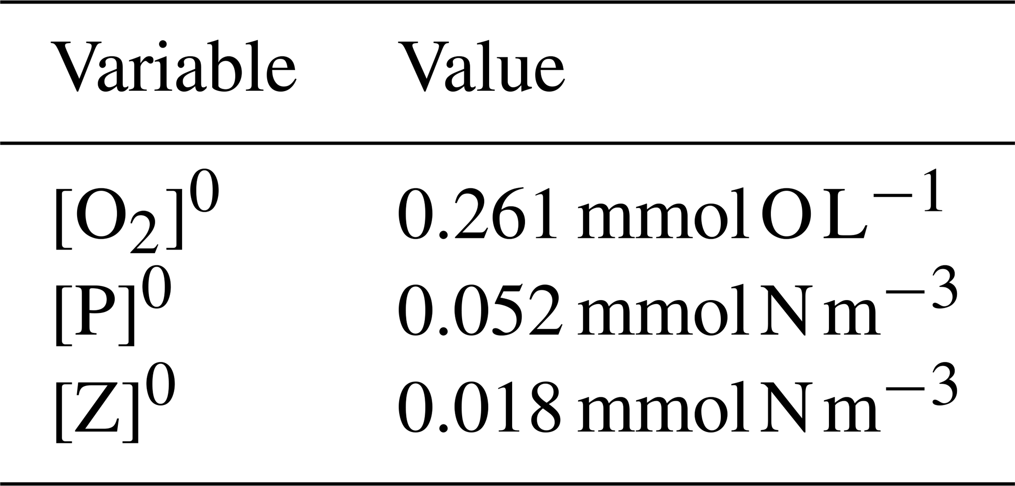
By varying the A, B and h parameters, the fixed point of the system can be made to approach X^w. Although other parameters may be varied instead of these three, we found that these are the ones whose variations are easier to judge in terms of displacement of the isoclines. This results in a coexistence fixed point X⁰ that is located near X^w, with coordinates shown in Table A2, which is a stable spiral point with eigenvalues of the Jacobian ${\mathit{\lambda }}_{\mathrm{1}}=-\mathrm{0.0847}$ and ${\mathit{\lambda }}_{\mathrm{2},\mathrm{3}}=-\mathrm{0.0009}\pm \mathrm{0.0221}i$.

Table A3 Parameters of the 0D SP2015 biogeochemical model.

Appendix B: Dynamics of the ECC simulation

We analyse the dynamics of the ECC simulation in terms of turbulent energy transfers, mean and eddy-induced circulations, and dominant turbulent length scales. Mean quantities refer to the alongshore average, e.g. for the cross-shore velocity u:

$$\begin{array}{}\text{(B1)}& \langle u(x,z,t)\rangle =L^{-\mathrm{1}}\int u(x,y,z,t)\mathrm{d}y,\end{array}$$

where L is the alongshore length of the channel. Perturbations are the departures from this mean: $u^{\prime }=u-\langle u\rangle$ and $\langle u^{\prime }\langle =\mathrm{0}$. The mean kinetic-energy transfer term is $c_{\mathrm{ke}}=-{\mathit{\rho }}_{\mathrm{0}}(\langle v_x\rangle \langle u^{\prime }{v}^{\prime }\rangle +\langle v_z\rangle \langle w^{\prime }{v}^{\prime }\rangle +\langle u_x\rangle \langle u^{\prime }{u}^{\prime }\rangle +\langle u_z\rangle \langle w^{\prime }{u}^{\prime }\rangle$), where ρ₀ is the reference density, v and w are the alongshore and vertical velocities, and a subscript denotes partial differentiation. The perturbation potential energy transfer term is $c_{\mathrm{pe}}=-g\langle w^{\prime }{\mathit{\rho }}^{\prime }\rangle$.

In the ECC case, c_pe remains positive, increasing after the wind intensification part of the wind cycle and decreasing when the wind relaxes (Fig. B1a), while c_ke oscillates between positive and negative values. The mechanism for c_ke growth seems to be the coalescence of disturbances into a single large eddy that is subsequently perturbed by rapidly emerging small-scale patterns (Durski and Allen, 2005). Anti-correlation between c_pe and c_ke is observable at days 35, 47, 53 and 60 (Fig. B1a), suggesting that c_ke evolution is related to nonlinear wave–wave interaction rather than to wave–mean flow interaction (Durski and Allen, 2005). For sustained winds, like the ECC wind cycle with short wind intensification and relaxation periods, the effects of this interaction were significant since the start of the simulations (Durski et al., 2007).

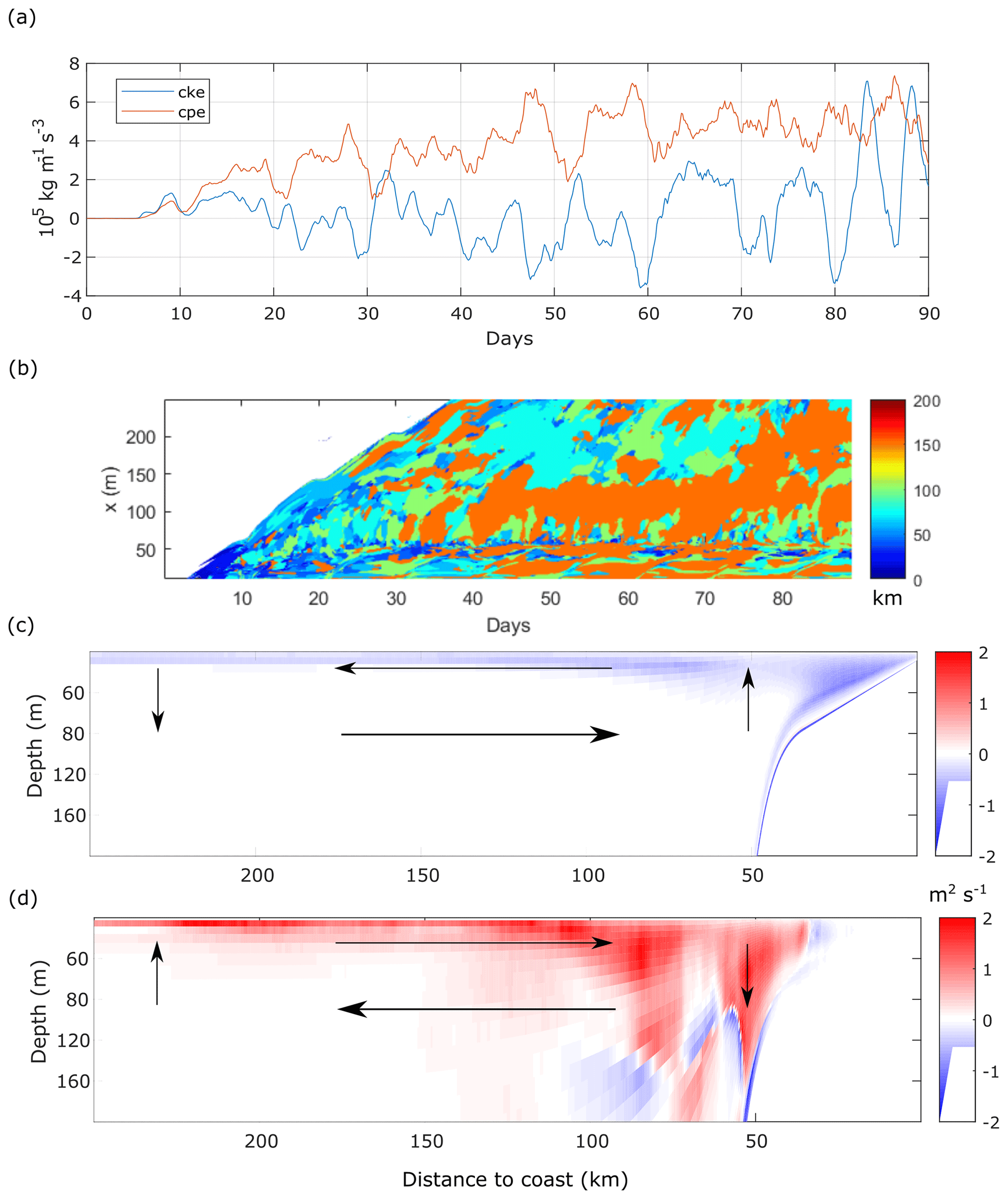
Figure B1 (a) Time series of the volume-averaged perturbation energy source terms of c_ke (green) and c_pe (blue). Volume average in the whole domain. (b) Peak wavelength of surface density anomaly alongshore wavenumber spectrum as a function of time and offshore distance. (c) Mean stream function over days 20 to 90. (d) Eddy stream function over days 20 to 90. Mean stratification is shown as black dash–dot contours in panels (c) and (d). Arrows in panels (c) and (d) represent a schematic view of the circulation.

Initially, the surface density peak length scale l_e, i.e. the most energetic scale, is homogeneous, and l_e is equal to the domain length (Fig. B1b).

Shortly after the start, small-scale (O(10 km)) fluctuations appear close to the shore, then grow in length and spread offshore. From day 20 onwards, l_e fully develops and ranges from 20 to 160 km across the shore, although until day 36 there are still regions where density is rather homogeneous.

Offshore the upwelling front (roughly from 50 km) we observe the emergence of two distinct regions in the cross-shore direction: a region adjacent to the front where large-scale structures are often dominant (l_e∼150–160 km) and further offshore where smaller-scale structures are dominant (l_e<100 km). The cross-shore extent of the first region appears to be related to the excursions in the c_ke time series (Fig. 3a), judging by the coincidence of the largest fluctuations of c_ke with the widest swaths of l_e∼150–160 km (days 45, 60, 68 and 80). The second region further offshore seldom exhibits l_e>100 km, as it is usually populated by filaments emerging from the front with contrasted density and by vortices resulting from the roll up of filament tips.

The wind-induced mean circulation in the x–z plane is $\mathrm{\Psi }=-\mathit{\tau }/{\mathit{\rho }}_{\mathrm{0}}f$, where τ is the applied wind stress and f is the Coriolis parameter. The eddy stream function is $\mathit{\psi }=(\langle v^{\prime }{b}^{\prime }\rangle \langle b_z^{\prime }\rangle -{\mathit{\lambda }}^{\mathrm{2}}\langle w^{\prime }{b}^{\prime }\rangle \langle b_y^{\prime }\rangle )/({\mathit{\lambda }}^{\mathrm{2}}\langle w^{\prime }{b}^{\prime }\rangle \langle b_y^{\prime }\rangle +\langle b_z^{\prime }\rangle )$, where b is buoyancy and λ=1000 is a stretching constant that accounts for the large aspect ratio of oceanic flows (Nagai et al., 2015; Plumb and Ferrari, 2005). The wind-induced mean circulation in the vertical cross-shore plane (Fig. B1c) is stronger at the surface and near the coast and weaker in the interior. A typical upwelling circulation is simulated: Ekman transport moves surface waters offshore and upwards near the coast, giving rise to the mean upward tilting of the isopycnals. The eddy-induced stream function (Fig. B1d) represents the component of the flow across the mean isopycnals (Cerovečki et al., 2009; Plumb and Ferrari, 2005), opposes the mean circulation and can surpass it. In agreement with Cerovečki et al. (2009) we find that the eddy stream function is stronger at the diabatic surface layer, in a thin layer (up to 20 m depth) with strong shoreward circulation 100 km offshore, deepening to 150 m at 75 km offshore. There is another strong eddy downwelling cell, on the shelf–slope transition, that goes down to 160 m depth.

The submesoscale and mesoscale turbulence is sustained by energy transfer from the potential energy field to the turbulent kinetic-energy field, through baroclinic conversion (Durski and Allen, 2005; Marchesiello et al., 2003). In agreement with previous modelling studies (Capet et al., 2008; Durski and Allen, 2005), the global picture is thus that the intermittent wind bursts act as a recharge for the mean potential energy which is then released to eddy kinetic energy through baroclinic instability. When the wind decreases, the eddy flux induces a rapid re-stratification of the upper layer (Capet et al., 2008).