Lyapunov analysis of multiscale dynamics: the slow bundle of the two-scale Lorenz 96 model

We investigate the geometrical structure of instabilities in the two-scale Lorenz 96 model through the prism of Lyapunov analysis. Our detailed study of the full spectrum of covariant Lyapunov vectors reveals the presence of a slow bundle in tangent space, composed by a set of vectors with a significant projection onto the slow degrees of freedom; they correspond to the smallest (in absolute value) Lyapunov exponents and thereby to the longer timescales. We show that the dimension of the slow bundle is extensive in the number of both slow and fast degrees of freedom and discuss its relationship with the results of a finite-size analysis of instabilities, supporting the conjecture that the slow-variable behavior is effectively determined by a nontrivial subset of degrees of freedom. More precisely, we show that the slow bundle corresponds to the Lyapunov spectrum region where fast and slow instability rates overlap, “mixing” their evolution into a set of vectors which simultaneously carry information on both scales. We suggest that these results may pave the way for future applications to ensemble forecasting and data assimilations in weather and climate models.

1 Introduction

Understanding the dynamics of multiscale systems is one of the great challenges in contemporary science, both for the theoretical aspects and the applications in many areas of interests for the society and the private sectors. Such systems are characterized by a dynamics that takes place on diverse spatial and/or temporal scales, with interactions between different scales combined with the presence of nonlinear processes. The existence of a variety of scales makes it hard to approach such systems using direct numerical integrations, since the problem is stiff. Additionally, simplifications based on naïve scale analysis, where only a limited set of scales are deemed important and the others are outright ignored, might be misleading or lead to strongly biased results. The nonlinear interaction with scales outside the considered range may, indeed, be important as a result of (possibly slow) upward or downward cascades of energy and information.

A crucial contribution to the understanding of multiscale systems comes from the now classic Mori–Zwanzig theory (Zwanzig, 1960, 1961; Mori et al., 1974), which allows one to construct an effective dynamics specialized for the scale of interest, which are, typically, the slow ones. The enthusiasm one may have for the Mori–Zwanzig formalism is partly counterbalanced by the fact that the effective coarse-grained dynamics is written in an implicit form so that it is of limited direct use. More tractable results can be obtained in the limit of an infinite timescale separation between the slow modes of interest and the very fast degrees of freedom one wants to neglect; in this case, the homogenization theory indicates that the effect of the fast degrees of freedom can be written as the sum of a deterministic, drift-like correction plus a stochastic white-noise forcing (Pavlioti and Stuart, 2008).

The climate provides an excellent example of a multiscale system, with dynamical processes taking place on a very large range of spatial and temporal scales. The chaotic, forced and dissipative dynamics and the nontrivial interactions between different scales represent a fundamental challenge in predicting and understanding weather and climate. A fundamental difficulty in the study of the multiscale nature of the climate system comes from the lack of any spectral gap, namely, a clear and well-defined separation of scales. The climatic variability covers a continuum of frequencies (Peixoto and Oort, 1992; Lucarini et al., 2014), so the powerful techniques based on homogenization theory cannot be readily applied.

On the other side, there is a fundamental need to construct efficient and accurate parametrizations for describing the impact of small scales on larger ones in order to improve our ability to predict weather and provide a better representation of climate dynamics. For some time it has been advocated that such parametrizations should include stochastic terms (Palmer and Williams, 2008). Such a point of view is becoming more and more popular in weather and climate modeling, even if the construction of parametrizations is mostly based on ad hoc, empirical methods (Franzke et al., 2015; Berner et al., 2017). Weather and climate applications have been instrumental in stimulating the derivation of new general results for the construction of parametrizations of multiscale systems and for understanding the scale–scale interactions. Recent advances have been obtained using the (i) Mori–Zwanzig and Ruelle response theory (Wouters and Lucarini, 2012, 2013), (ii) the generalization of the homogenization-theory-based results obtained via the Edgeworth expansion (Wouters and Gottwald, 2017), and (iii) the use of hidden Markov layers (Chekroun et al., 2015a, b) from a data-driven point of view. An extremely relevant possible advantage of using theory-based methods is the possibility of constructing scale-adaptive parametrizations (see discussion in Vissio and Lucarini, 2017, ;).

Another angle on multiscale systems deals with the study of the scale–scale interactions, which are key in understanding instabilities and dissipative processes and the associated predictability and error dynamics. Lyapunov exponents (Pikovsky and Politi, 2016), which describe the linearized evolution of infinitesimal perturbations, are mathematically well-established quantities and seem to be the most natural choice to start addressing this problem. However, as it is well known in multiscale systems, the maximum (or leading) Lyapunov exponent controls only the early-stage dynamics of very small perturbations (Lorenz, 1996). As time goes on, the amplitude of the perturbations of the fastest variables start saturating, while those affecting the slowest degrees of freedom grow at a pace mostly controlled by the (typically weaker) instabilities characteristic of the slower degrees of freedom. While nonlinear tools, such as finite-size Lyapunov exponents (Aurell et al., 1997), are able to capture the rate of this multiscale growth, they lack the mathematical rigor of infinitesimal analysis. In particular, they are unable to convey information on the leading directions of these perturbations when they grow across multiple scales – an essential problem if one wishes to investigate, at a deterministic level, the nontrivial correlations across structures and perturbations acting on different scales. It is therefore of primary importance to better understand the multiscale and interactive structure of these instabilities and, in particular, to probe the sensitivity of multiscale systems to infinitesimal perturbations acting at different spatial and temporal scales and different directions. To this purpose, infinitesimal Lyapunov analysis allows one to compute not only a full spectrum of Lyapunov exponents (LEs) but also their corresponding tangent-space directions, the so-called covariant Lyapunov vectors (CLVs; Ginelli et al., 2007). CLVs are associated with LEs (in a relationship that, loosely speaking, resembles the eigenvector–eigenvalue pairing) and provide an intrinsic decomposition of tangent space that links growth (or decay) rates of (small) perturbations to physically based directions in configuration space. In principle, they can be used to associate instability timescales (the inverse of LEs) with well-defined real-space perturbations or uncertainties.

While this information is gathered at the linearized level, one may nevertheless conjecture that LEs and CLVs associated with the slowest timescales (i.e., the smallest LEs in absolute value) can capture relevant information on the large-scale dynamics and its correlations with the faster degrees of freedom. In a sense, one may conjecture that the small LEs and the corresponding CLVs could be used to gain access to a nontrivial effective large-scale dynamics. See, for instance, Norwood et al. (2013), where three coupled Lorenz 63 systems are investigated. Accordingly, the identification of linear instabilities in full multiscale models is then expected to have practical implications in terms of control and predictability. In the following, we will begin to investigate these ideas, studying the tangent-space structure of a simple two-scale atmospheric model, the celebrated Lorenz 96 (L96) model first introduced in Lorenz (1996).

The L96 model provides a simple yet prototypical representation of a two-scale system where large-scale, synoptic variables are coupled to small-scale, convective variables. The Lorenz 96 model was quickly established as an important test bed for evaluating new methods of data assimilation (Trevisan and Uboldi, 2004; Trevisan et al., 2010) and stochastic-parametrization schemes (Vissio and Lucarini, 2017; Orrel, 2003; Wilks, 2006). In the latest decade, it also received considerable attention in the statistical physics community (Abramov and Majda, 2007; Hallerberg et al., 2010; Lucarini and Sarno, 2011; Gallavotti and Lucarini, 2014), while an earlier study – limited to the stronger instabilities – highlighted the localization properties of the associated CLVs (Herrera et al., 2011).

Our Lyapunov analysis reveals the existence of a nontrivial slow bundle in tangent space, formed by a set of CLVs – associated with the smallest LEs – that was the only one with a nonnegligible projection onto the slow variables. The number of these CLVs is considerably larger than the number of slow variables, and it is extensive in the number of slow and fast degrees of freedom. At the same time, the directions associated with highly expanding and contracting LEs are aligned almost exclusively along the fast, small-scale degrees of freedom. Moreover, we show that the LE corresponding to the first CLV of the slow bundle (i.e., the most expanding direction within this subspace) approaches the finite-size Lyapunov exponent in a large-perturbation range, where linearization is not generally expected to apply.

Altogether, it should be made clear that the timescale separation between the slow bundle and the fast degrees of freedom is large but finite and stays finite when the number of degrees of freedom is let to diverge (i.e., it is not a standard hydrodynamics component). Additionally, the stability is not absolutely weak in the sense of nearly vanishing Lyapunov exponents.

The paper is organized as follows. Section 2 introduces both the L96 model and the fundamental tools of the Lyapunov analysis used in this paper. Evidence for the existence of a slow bundle is presented in Sect. 3. In Sect. 4, we investigate how this slow structure arises from the superposition of the instabilities of the slow and fast dynamics. Section 5, on the other hand, is devoted to a comparison with results of finite-size analysis. Finally, in Sect. 6 we discuss our results, further commenting on their generality and proposing future developments and applications.

2 The Lorenz 96 model: a simple multiscale system

2.1 Model definition and scaling considerations

The L96 model is a simple example of an extended multiscale system such as the Earth atmosphere. Its dynamics is controlled by synoptic variables, characterized by a slow evolution over large scales, coupled to the so-called convective variables characterized by a faster dynamics over smaller scales.

The synoptic variables X_k, with $k=\mathrm{1},\mathrm{\dots },K$, represent generic observables on a given latitude circle; each X_k is coupled to a subgroup of J convective variables Y_k,j ($j=\mathrm{1},\mathrm{\dots },J$) that follow the faster convective dynamics typical of the k sector,

$$\begin{array}{ll}\text{(1a)}& {\displaystyle }{\dot{X}}_k& {\displaystyle }=X_{k-\mathrm{1}}(X_{k+\mathrm{1}}-X_{k-\mathrm{2}})-X_k+F_{\mathrm{s}}-{\displaystyle \frac{hc}{b}}\sum _j{Y}_{k,j},{\displaystyle }{\dot{Y}}_{k,j}& {\displaystyle }=cb{Y}_{k,j+\mathrm{1}}(Y_{k,j-\mathrm{1}}-Y_{k,j+\mathrm{2}})-c{Y}_{k,j}\\ \text{(1b)}& {\displaystyle }& {\displaystyle }+{\displaystyle \frac{c}{b}}{F}_{\mathrm{f}}+{\displaystyle \frac{hc}{b}}{X}_k.\end{array}$$

In both sets of equations, the nonlinear nearest-neighbor interaction provides an account of advection due to the movement of air masses, while the last terms describe the mutual coupling between the two sets of variables. Each X_k variable is affected by the sum of the associated Y_k,j variables, while each Y_k,j is forced by the variable X_k corresponding to the same sector k. Finally, the linear terms −X_k and $-c{Y}_{k,j}$ account for internal dissipative processes (viscosity) and are responsible for the contractions of the phase space.

We remark that in our configuration, following Vissio and Lucarini (2017), energy is injected in the system both at large and at small scales, provided by the constant terms F_s and F_f, which impact the slow and fast scales of the system, respectively.

The presence of the additional forcing term acting on the Y_k,j variables makes it possible to have chaotic dynamics on the small scales also in the limit of vanishing coupling (h→0), as opposed to the typical L96 setting, where the small-scale variables become spontaneously chaotic without the need of being forced by their associated X_k as a result of downward energy cascade from the slow variables.

Moreover, the parameter c controls the timescale separation between the X_k and Y_k,j variables, while b controls the relative amplitude of the Y_k,j components. Finally, h gauges the strength of the coupling between slow and fast variables.

The L96 model thus contains K slow variables and K×J fast variables for a total of $N=K(\mathrm{1}+J)$ degrees of freedom. It is complemented by the boundary conditions

$$\begin{array}{ll}{\displaystyle }& {\displaystyle }{X}_{k-K}=X_{k+K}=X_k,\\ {\displaystyle }& {\displaystyle }{Y}_{k-N,j}=Y_{k+K,j}=Y_{k,j},\\ {\displaystyle }& {\displaystyle }{Y}_{k,j-J}=Y_{k-\mathrm{1},j},\\ \text{(2)}& {\displaystyle }& {\displaystyle }{Y}_{k,j+J}=Y_{k+\mathrm{1},j}.\end{array}$$

In his original work (Lorenz, 1996), Edward Lorenz considered K=36 slow variables and J=10 fast variables for each subsector, for a total of N=396 degrees of freedom. As usual, one is ideally interested in dealing with arbitrarily large K and J values, so it is preferable to formulate the model in such a way that it remains meaningful in the limit $K,J\to \mathrm{\infty }$. In this respect, the only potential problem is the global coupling, represented by the sum in Eq. (1a), which should stay finite for J→∞. This can be easily ensured by setting the coefficient in front of the sum to be inversely proportional to J. The most compact representation is obtained by introducing the rescaled variables $Z_{k,j}=b{Y}_{k,j}$ and replacing b with a new parameter f:

$$\begin{array}{}\text{(3)}& f={\displaystyle \frac{Jc}{b^{\mathrm{2}}}}.\end{array}$$

With these transformations, Eqs. (1a) and (1b) can be rewritten as

$$\begin{array}{ll}\text{(4a)}& {\displaystyle }& {\displaystyle }{\dot{X}}_k=X_{k-\mathrm{1}}(X_{k+\mathrm{1}}-X_{k-\mathrm{2}})-X_k+F_{\mathrm{s}}-hf{〈Z_{k,j}〉}_j,{\displaystyle }& {\displaystyle \frac{\mathrm{1}}{c}}{\dot{Z}}_{k,j}=Z_{k,j+\mathrm{1}}(Z_{k,j-\mathrm{1}}-Z_{k,j+\mathrm{2}})-Z_{k,j}\\ \text{(4b)}& {\displaystyle }& {\displaystyle }+F_{\mathrm{f}}+h{X}_k,\end{array}$$

where

$$\begin{array}{}\text{(5)}& {〈Z_{k,j}〉}_j={\displaystyle \frac{\mathrm{1}}{J}}\sum _{j=\mathrm{1}}^J{Z}_{k,j},\end{array}$$

while the boundary conditions are the same as above. In practice f gauges the asymmetry of the interaction between slow and fast variables. From its definition, it is clear that f strongly depends on the scale separation b. For the standard choice of the parameter values (see below), f=1, i.e., the average influence of the fast scales on the slow ones is the same as the opposite. On the other hand, if we increase the value of b, f→0, which corresponds to a master–slave limit, where the fast variables do not affect the slow ones but are actually slaved to them. This makes sense because the small-scale variables have extremely small amplitude. The opposite master–slave limit, perhaps more interesting from a climatological point of view, corresponds to taking the h→0 and f→∞ limits, while keeping the product hf constant. In this case, the fast variables follow up to first approximation their own autonomous dynamics but still drive the slow ones through the finite coupling term $hf{〈Z_{k,j}〉}_j$. In this latter limit, we envision the presence of an upscale energy transfer.

Apart from helping to clarify these master–slave limiting cases, such a reformulation of the model also allows us to better understand that, in order to maintain a fixed amplitude of the coupling term, it is necessary to keep f constant when J is varied. Selecting a constant value for the timescale separation c, we choose to rescale b with J as follows:

$$\begin{array}{}\text{(6)}& b=\sqrt{{\displaystyle \frac{Jc}{f}}}.\end{array}$$

With reference to the Lorenz original parameter choices (Lorenz, 1996), $b=c=\mathrm{10}$ and J=10, we have f=1 and the suggested scaling,

$$\begin{array}{}\text{(7)}& b=\sqrt{\mathrm{10}J}.\end{array}$$

It is finally interesting to note that, in the absence of forcing and dissipation, Eqs. (1a) and (1b) reduce to

$$\begin{array}{}\text{(8a)}& {\displaystyle }& {\displaystyle }{\dot{X}}_k=X_{k-\mathrm{1}}(X_{k+\mathrm{1}}-X_{k-\mathrm{2}})-{\displaystyle \frac{hc}{b}}\sum _j{Y}_{k,j},\text{(8b)}& {\displaystyle }& {\displaystyle }{\dot{Y}}_{k,j}=cb{Y}_{k,j+\mathrm{1}}(Y_{k,j-\mathrm{1}}-Y_{k,j+\mathrm{2}})+{\displaystyle \frac{hc}{b}}{X}_k,\end{array}$$

which conserve a quadratic form of slow and fast variables (Vissio and Lucarini, 2017),

$$\begin{array}{}\text{(9)}& E=\sum _k{X}_k^{\mathrm{2}}+\sum _{k,j}{Y}_{k,j}^{\mathrm{2}}=\sum _k\left(X_k^{\mathrm{2}}+{\displaystyle \frac{f}{c}}{〈Z_{k,j}^{\mathrm{2}}〉}_j\right).\end{array}$$

This conservation law, of course, does not hold in the more interesting forced and dissipative case. However, this result suggests that E can be identified with a bona fide energy – and represents a natural norm – also in the forced and dissipative case. Note also that, according to the last equality in Eq. (9), changing the number of fast variables does not change the total energy budget, provided that the ratio f∕c remains constant.

Given the more natural definition of the energy, when expressed in terms of the Y variables, in the following we keep using the original Lorenz notations, denoting the slow variables with the letter Y. Moreover, unless otherwise specified, we will implicitly consider f=1 and typically adopt the slow forcing and the timescale separation originally adopted by Lorenz, F_s=10 and c=10, and choose values for b and J that satisfy the scaling condition (7). According to Lorenz's original derivation, one time unit in this model dynamics is roughly equivalent to 5 d in the real climate evolution (Lorenz, 1996).

We will fix F_f=6, which guarantees chaoticity in the uncoupled fast variables in the absence of coupling. Lorenz's original choice for the coupling between the slow and fast scales was h=1, but here we will also explore the weak coupling regime, considering coupling values as small as $h=\mathrm{1}/\mathrm{16}$.

2.2 Elements of Lyapunov analysis: Lyapunov exponents and covariant Lyapunov vectors

As mentioned above, the right tools to quantify rigorously the rate of divergence (or convergence) of nearby trajectories are the LEs and their associated covariant CLVs. We provide here a qualitative description of these objects. For a more thorough discussion, the reader can look to Ruelle (1979), Eckmann and Ruelle (1985), Ginelli et al. (2013), and Kuptsov and Parlitz (2012) and references therein.

For definiteness, let us consider an N-dimensional continuous-time dynamical system,

$$\begin{array}{}\text{(10)}& \dot{\mathit{x}}\left(t\right)=\mathit{f}\left(\mathit{x}\right(t\left)\right),\end{array}$$

with x(t) being the state of the system at time t. One can linearize the dynamics around a given trajectory, thus obtaining the evolution of an infinitesimal perturbation δx(t) in the so-called tangent space:

$$\begin{array}{}\text{(11)}& \mathit{\delta }\dot{\mathit{x}}\left(t\right)=\mathbf{J}(\mathit{x},t)\mathit{\delta }\mathit{x}\left(t\right),\end{array}$$

where we have introduced the Jacobian matrix

$$\begin{array}{}\text{(12)}& \mathbf{J}(\mathit{x},t)={\displaystyle \frac{\partial \mathit{f}\left(\mathit{x}\right(t\left)\right)}{\partial \mathit{x}\left(t\right)}}.\end{array}$$

LEs λ_i measure the (asymptotic) exponential rates of growth (or decay) of infinitesimal perturbations along a given trajectory. Their plurality holds in the fact that the growth rates associated with different directions of the infinitesimal perturbations are in general different. We then refer to the ordered sequence ${\mathit{\lambda }}_{\mathrm{1}}\ge {\mathit{\lambda }}_{\mathrm{2}}\ge \mathrm{\dots }\ge {\mathit{\lambda }}_N$ as the spectrum of characteristic LEs, or the Lyapunov spectrum (LS), with N being the dimension of the dynamical system. At each point x(t) of the attractor, the CLVs v_i(x(t)) give the directions of growth of perturbations associated with the corresponding Lyapunov exponent¹. In other words, they span the Oseledets splitting (Eckmann and Ruelle, 1985), i.e., an infinitesimal perturbation δx_i(t₀) exactly aligned with the ith CLV v_i(x(t₀)), and after a sufficiently long time, t will grow or decay as

$$\begin{array}{}\text{(13)}& ∥\mathit{\delta }{\mathit{x}}_i(t_{\mathrm{0}}+t)∥\approx ∥\mathit{\delta }{\mathit{x}}_i\left(t_{\mathrm{0}}\right)∥e^{{\mathit{\lambda }}_{i}t}.\end{array}$$

LEs are global quantities, measuring the average exponential growth rate along the attractor, while CLVs are local objects, defined at each point of the attractor and transforming covariantly along each trajectory, according to the linearized dynamics (11),

$$\begin{array}{}\text{(14)}& \mathit{v}\left(\mathit{x}\right(t\left)\right)=\mathbf{M}({\mathit{x}}_{\mathrm{0}},t)\mathit{v}\left({\mathit{x}}_{\mathrm{0}}\right),\end{array}$$

where x₀≡x(0) and the tangent linear propagator M(x₀,t) satisfies

$$\begin{array}{}\text{(15)}& \dot{\mathbf{M}}({\mathit{x}}_{\mathrm{0}},t)=\mathbf{J}(\mathit{x},t)\mathbf{M}({\mathit{x}}_{\mathrm{0}},t),\end{array}$$

with M(x₀,0) being the identity matrix.

In the following, we always refer to CLVs assuming that they have been properly normalized. With the above-mentioned exception of degeneracies, CLVs constitute an intrinsic (they do not depend on the chosen norm) tangent-space decomposition into the stable and unstable directions associated with the different LEs. LEs themselves have units of inverse time so that the largest positive (in absolute value) exponents – and their associated CLVs – describe fast growing (or contracting) perturbations, while the smaller ones correspond to longer timescales.

Unfortunately, Eqs. (13)–(14) cannot be used to directly compute any LEs or CLVs beyond the first one. Unavoidable numerical errors generated while handling higher-order CLVs are amplified according to a rate dictated by the largest LE so that any tangent-space vector quickly converges to the first CLV. In order to avoid this collapse, it is customary to periodically orthonormalize the vectors with a QR decomposition (Shimada and Nagashima, 1979; Benettin et al., 1980). LEs are thereby computed as the logarithms of the basis vector normalization factors, time averaged along the entire trajectory.

The mutually orthogonal vectors, obtained as a by-product of this procedure, constitute a basis in tangent space and are usually referred to as Gram–Schmidt vectors (by the name of the algorithm used to perform the QR decomposition) or backward Lyapunov vectors (BLVs; because they are obtained by integrating the system forward until a given point in time, thus spanning the past trajectory with respect to this point). Being forced to be mutually orthogonal, BLVs allow only reconstructing the orientation of the subspaces spanned by the most expanding directions. In this work, we concentrate on the CLVs for the identification of the various expanding and/or contracting directions. This is done by implementing a dynamical algorithm based on a clever combination of both forward and backward iterations of the tangent dynamics, introduced in Ginelli et al. (2007) and more extensively discussed in Ginelli et al. (2013).

In practice, one first evolves the forward dynamics, following a phase-space trajectory to compute the full LS $\mathit{\{}{\mathit{\lambda }}_i{\mathit{\}}}_{i=\mathrm{1},\mathrm{\dots },N}$ and the basis of BLVs $\mathit{\left\{}{\mathit{g}}_i\right(t_m){\mathit{\}}}_{i=\mathrm{1},\mathrm{\dots },N}$ with a series of QR decompositions performed along the trajectory for every τ time unit, at times t_m=mτ, with $m=\mathrm{1},\mathrm{\dots },M$. One is then left with a series of orthogonal matrices Q_m, whose columns are the BLVs g_i(t_m), and the upper triangular matrices R_m which contain the vector norms and their mutual projections.

The key idea is then to project a generic tangent-space vector u(t_m) on the covariant subspaces S_j(t_m) spanned by the first j BLVs at times t_m. It can be easily shown (Ginelli et al., 2013) that this projection, evolved backward in time according to the inverse tangent-space dynamics, converges exponentially quickly to the jth covariant vector². In practice, this backward procedure can be performed by expressing the CLVs in the BLVs basis,

$$\begin{array}{}\text{(16)}& {\mathit{v}}_j\left(t_m\right)=\sum _{i=\mathrm{1}}^j{c}_{i,j}\left(t_m\right){\mathit{g}}_i\left(t_m\right).\end{array}$$

The coefficients c_i,j(t_m) thus compose an upper triangular matrix C_m, whose dynamics is actually determined by the R_m matrices obtained from the QR decomposition

$$\begin{array}{}\text{(17)}& {\mathbf{C}}_m={\mathbf{R}}_m{\mathbf{C}}_{m-\mathrm{1}}.\end{array}$$

This last relationship is easily invertible, assuring a computationally efficient and precise method to follow the backward dynamics.

2.3 Lorenz 96 tangent-space dynamics and algorithmic aspects

The tangent-space dynamics of L96 can be readily obtained by linearizing the phase-space evolution Eqs. (1a) and (1b),

$$\begin{array}{ll}{\displaystyle }\mathit{\delta }{\dot{X}}_k& {\displaystyle }=\mathit{\delta }{X}_{k-\mathrm{1}}(X_{k+\mathrm{1}}-X_{k-\mathrm{2}})\\ {\displaystyle }& {\displaystyle }+X_{k-\mathrm{1}}(\mathit{\delta }{X}_{k+\mathrm{1}}-\mathit{\delta }{X}_{k-\mathrm{2}})-\mathit{\delta }{X}_k\\ \text{(18a)}& {\displaystyle }& {\displaystyle }-{\displaystyle \frac{hc}{b}}\sum _j\mathit{\delta }{Y}_{k,j},{\displaystyle }\mathit{\delta }{\dot{Y}}_{k,j}& {\displaystyle }=cb\left[\mathit{\delta }{Y}_{k,j+\mathrm{1}}\right(Y_{k,j-\mathrm{1}}-Y_{k,j+\mathrm{2}})\\ {\displaystyle }& {\displaystyle }+Y_{k,j+\mathrm{1}}(\mathit{\delta }{Y}_{k,j-\mathrm{1}}-\mathit{\delta }{Y}_{k,j+\mathrm{2}})]-c\mathit{\delta }{Y}_{k,j}\\ \text{(18b)}& {\displaystyle }& {\displaystyle }+{\displaystyle \frac{hc}{b}}\sum _j\mathit{\delta }{X}_k,\end{array}$$

where δX_k and δY_k,j are infinitesimal perturbations of, respectively, slow and fast variables. Together, they define the tangent-space vector $\mathit{u}\equiv (\mathit{\delta }{X}_{\mathrm{1}},\mathrm{\dots },\mathit{\delta }{X}_K,\mathit{\delta }{Y}_{\mathrm{1},\mathrm{1}},\mathrm{\dots }\mathit{\delta }{Y}_{K,J})$. One can easily deduce the Jacobian matrix from Eqs. (18a) and (18b).

In this paper, we numerically integrate Eqs. (1a), (1b), (18a) and (18b) using a Runge–Kutta fourth-order algorithm with a time step $\mathrm{\Delta }t={\mathrm{10}}^{-\mathrm{3}}$, shorter than the choice $\mathrm{\Delta }t=\mathrm{5}\times {\mathrm{10}}^{-\mathrm{3}}$ typically made for the standard L96 model. In fact, we have verified that such a small time step is actually required in order to compute the entire spectrum of LEs and CLVs with sufficient accuracy. Typically, to discount transient effects in numerical simulations, we discard the first 10³ time units, split in two equal parts: the first 500 time units allow for the phase-space trajectory to reach its attractor, while the second is used for the convergence of the tangent-space vectors towards the BLVs basis. Afterwards, a forward integration of typically T=10³ time units is performed in order to analyze the properties of tangent space. Due to the highly unstable nature of the L96 model (we will see in the following that the maximum LE is around 20 for our choice of parameter values), we have to perform the tangent-space orthonormalization every $\mathit{\tau }={\mathrm{10}}^{-\mathrm{2}}$ time unit. Finally, a transient of 10² time units is used during the backward dynamics to ensure the convergence of the backward vectors to the true CLVs. We have also carefully verified that the forward and backward transients are long enough to guarantee a sufficiently accurate convergence to the true LEs and CLVs.

2.4 The Lorenz 96 Lyapunov spectrum

Spatially extended systems are known to typically exhibit an extensive Lyapunov spectrum (Ruelle, 1978; Livi et al., 1986; Grassberger, 1989). This property is instrumental for the identification of intensive and extensive observables in the thermodynamic sense. Extensivity means that for N tending to infinity (i.e., in the so-called thermodynamic limit), the spectrum λ_i is a function of the rescaled index $\mathit{\rho }=i/N$ only³.

Figure 1 Extensivity of chaos. (a) Lyapunov spectra as functions of the rescaled index $i_{\mathrm{r}}=(i-\mathrm{1}/\mathrm{2})/N$ for K=18, 24 and 36 and J=10, 15, 20, 25 and 30 (all possible combinations). (b) Details of the central region $i_{\mathrm{r}}\in (\mathrm{0.45},\mathrm{0.55})$. The cyan arrow marks the direction of increasing J values, while each J branch is the superposition of the spectra for K=18 (circles), K=24 (squares) and K=36 (triangles). Inset of panel (a): Kolmogorov–Sinai entropy H_KS (black circles) and Kaplan–Yorke dimension d_KY (red squares) as a function of the number of degrees of freedom $N=K(J+\mathrm{1})$. The dashed lines mark a linear fit with zero intercept and slope ≈2.6 (H_KS) and ≈0.7 (d_KY). Simulations have been performed with h=1 and $b=\sqrt{\mathrm{10}J}$ (see main text).

The single-scale L96 model (i.e., Eq. 1a) without the coupling to the fast scale) is no exception (Karimi and Paul, 2010; Gallavotti and Lucarini, 2014). Here we show that extensivity of chaotic behavior holds also in the two-scale model provided that – as discussed in Sect. 2.1 – the relation (6) is satisfied. In the present context, the total number N of degrees of freedom is controlled by two separate indicators, K and J, so that, in principle, one can define two distinct thermodynamic limits, i.e., K→∞ and J→∞. However, in practice, as long as $K,J\gg \mathrm{1}$, the spectral shape depends only on N alone, as seen in Fig. 1, where several different LSs nicely overlap.

In order to appreciate the different role of K and J, it is necessary to zoom in, as shown in Fig. 1b, where the region characterized by a larger spread is displayed. The single spectra are grouped into five different branches, each corresponding to three different values of K (K=18, 24 and 36, respectively marked as circles, squares and triangles) and to the same J. As J increases from 10 to 30, these branches converge to a limiting spectrum, which corresponds to the double thermodynamic limit $K,J\to \mathrm{\infty }$. The indistinguishability of the spectra obtained for the same J shows that K-type finite-size corrections are very small for the given K; this is not a surprise, since the number of fast variables, KJ, is much larger than that of the slow variables, K.

The existence of a limit spectrum implies that the Kolmogorov–Sinai entropy H_KS – a measure of the diversity of the trajectories generated by the dynamical system – is proportional to the number N of degrees of freedom. This can be appreciated in the inset of Fig. 1a (see the black circles), where H_KS is determined through the Pesin formula, which provides an upper bound to H_KS (Eckmann and Ruelle, 1985),

$$\begin{array}{}\text{(19)}& H_{\mathrm{KS}}=\sum _{\mathit{\lambda }>\mathrm{0}}{\mathit{\lambda }}_i.\end{array}$$

Similarly, the dimension of the attractor, i.e., the number of “active” degrees of freedom, is proportional to N, as seen again from Fig. 1a, where we have plotted the Kaplan–Yorke dimension D_KY (see red squares; Eckmann and Ruelle, 1985):

$$\begin{array}{}\text{(20)}& D_{\mathrm{KY}}=M+{\displaystyle \frac{{\sum }_{i\le M}{\mathit{\lambda }}_i}{\left|{\mathit{\lambda }}_{M+\mathrm{1}}\right|}},\end{array}$$

with M being the largest integer such that ${\sum }_i{\mathit{\lambda }}_i>\mathrm{0}$.

Figure 2 (a) Lyapunov spectrum for the conservative setup in Eqs. (8a) and (8b). Parameters are b=10, K=36 and J=10 (N=396 LEs), and initial conditions are chosen such that the conserved energy is E=36. The black solid line corresponds to h=1, while the dashed green line corresponds to $h=-\mathrm{1}$; in the inset, the absolute difference Δλ_i between the two LSs is compared with one standard error in our numerical estimate (blue dashed line). (b) The second half of the Lyapunov spectrum ($i\in [\mathrm{199},\mathrm{396}]$; red dashed line) is folded under the reflection transformation ${\mathit{\lambda }}_i\to -{\mathit{\lambda }}_{N-i+\mathrm{1}}$ over its first half ($i\in [\mathrm{1},\mathrm{198}]$; black solid line); in the inset, the absolute difference Δλ_i between LS and its folded transformation is compared with one standard error in our numerical estimate (dashed blue line).

We conclude this section with a brief remark on the Lyapunov spectrum in the zero-dissipation limit (8a and 8b), shown in Fig. 2a for h=1. The LS depends only on the initial value of the energy of the system (in our simulations, we have chosen E=36 – see Eq. 9)⁴. Moreover, from Fig. 2b, we can appreciate that the LS is perfectly symmetric, since the second half of the spectrum superposes to the first half under the transformation ${\mathit{\lambda }}_i\to -{\mathit{\lambda }}_{N-i+\mathrm{1}}$ within numerical precision. This symmetry is an unexpected general property, which holds for any choice of h, c and b. In fact, the conservation law can only account for the existence of an extra zero-Lyapunov exponent. The overall symmetry of the LS must follow from more general properties such as the symplectic structure of the model or invariance under time reversal of the evolution equations. Unfortunately, this model is known to possess no symplectic structure, even if the energy is conserved (Blender et al., 2013), and the only symmetry we have been able to find is the invariance under the transformation $t\to -t$, $X_k\to -X_k$ and $Y_{k,j}\to -Y_{k,j}$, accompanied by a change of the coupling constant h. Indeed, the green dashed line in Fig. 2a shows that the Lyapunov spectrum is invariant under the transformation $h\to -h$. Therefore, the overall symmetry remains an unexplained property.

3 Slow tangent-space bundle

3.1 Projection of CLVs in the X subspace

We now come to the central result of this paper, namely the existence of a nontrivial subspace in tangent space associated with the slow dynamics of the L96 model.

The individual LEs λ_i represent the average growth rate (and thus the inverse of suitable timescales) of well-defined small perturbations aligned along the corresponding CLV, v_i. It is therefore logical to ask which of these “fundamental” perturbations are more relevant for the evolution of the accessible macroscopic observables. In the present case, it is natural to focus our attention on the alignment along the slow variables X_k.

The norm of the (rescaled) ith CLV can be written as

$$\begin{array}{}\text{(21)}& \left|\right|\mathit{\delta }{X}^{\left(i\right)}|{|}^{\mathrm{2}}+|\left|\mathit{\delta }{Y}^{\left(i\right)}\right|{|}^{\mathrm{2}}=\mathrm{1},\end{array}$$

where the two addenda represent the squared Euclidean norm of the projection onto the slow and fast variables, $\mathit{\delta }{X}^{\left(i\right)}=(\mathit{\delta }{X}_{\mathrm{1}}^{\left(i\right)},\mathrm{\dots },\mathit{\delta }{X}_K^{\left(i\right)})$ and $\mathit{\delta }{Y}^{\left(i\right)}=(\mathit{\delta }{Y}_{\mathrm{1},\mathrm{1}}^{\left(i\right)},\mathrm{\dots }\mathit{\delta }{Y}_{K,J}^{\left(i\right)})$, respectively. The most natural indicator of how much the ith CLV projects on the slow modes is thus the X-projected norm ${\mathit{\varphi }}_i\equiv \left|\right|\mathit{\delta }{X}^{\left(i\right)}|{|}^{\mathrm{2}}$.

However, it should be noted that, although the CLVs are intrinsic vectors, their mutual angles do depend on the relative scales used to represent the single variables and, in particular, fast and slow ones. If we change the units of measure used to quantify the fast Y variables, introducing V_j=γY_j, the (Euclidean) norm of the ith CLV becomes

$$L={\mathit{\varphi }}_i+{\mathit{\gamma }}^{\mathrm{2}}(\mathrm{1}-{\mathit{\varphi }}_i).$$

As a result, in the new representation, the weight of the projection onto the slow variables becomes

$${\mathit{\varphi }}_i^{\prime }={\displaystyle \frac{{\mathit{\varphi }}_i}{L}},$$

which shows how the amplitude of the projection depends on the relative scale used to measure fast and slow variables. Since in the very definition of energy (see Eq. 9), X and Y variables are weighted in the same way, it is natural to maintain the original definition, i.e., to assume that γ=1. Nevertheless, as we will see while discussing the evolution of finite perturbations, the relative scale is an important parameter we can play with to extract useful information.

Given the strong temporal fluctuations of ϕ_i(t) when the vectors are covariantly transformed along a trajectory (see the end of this section), it is convenient to refer to its time average (which, assuming ergodicity, corresponds to an ensemble average over the invariant measure),

$$\begin{array}{}\text{(22)}& {\mathrm{\Phi }}_i=\langle {\mathit{\varphi }}_i\left(t\right){\rangle }_t.\end{array}$$

We have first computed the projection norm Φ_i for the entire spectrum of vectors in a system of size K=36 and J=10 with the “standard” parameter value b=10. In a wide range of coupling strengths – from strong (h=1) to weak ($h=\mathrm{1}/\mathrm{16}$) – we find that both rapidly growing and rapidly contracting perturbations are almost orthogonal to the slow-variable subspace, the associated CLVs exhibiting a negligible projections over the X directions (see Fig. 3a). In fact, only a “central band” constituted by the CLVs associated with the smallest LEs displays a significative projection over the slow variables. Note, however, that the typical LEs associated with the central band CLVs are clearly finite and are deemed “small” only in a relative sense, i.e., when compared with the largest positive and negative exponents of the full spectrum. For instance, for $h=\mathrm{1}/\mathrm{4}$, we can approximately estimate the corresponding portion of the LS to extend between a magnitude of 2 and −5. We will comment further on this point in Sect. 4.

Note also that the CLV associated with the only null LE (in the following we simply denote it as the 0-CLV) displays a sharp peak of the projection norm Φ_i. This is just a consequence of the delocalization of this CLV: the perturbation corresponding to the zero exponent points exactly along the trajectory. Direct integration of the phase-space equations (not shown) confirms that the total variability of the slow variables is of the same order of magnitude as the total variability of the fast ones. This central band of CLVs defines the tangent-space slow bundle relevant for this paper. It becomes more sharply defined for small values of the coupling h, but it keeps approximately the same position and width as the coupling h is increased. In particular, for this set of parameter values, this nontrivial slow bundle extends in tangent space over roughly 120 CLVs, much more than the K=36 slow degrees of freedom. The extension of the slow bundle can be better appreciated in Fig. 3b, where the time-averaged projections are shown on the logarithmic scale (top part of panel) and compared with the full spectrum of LEs (bottom part of panel).

Figure 3 CLV projection onto the slow variables. (a) CLV average projection norm Φ_i of the CLVs (see text) as a function of the vector index for K=36, J=10 and b=10 upon varying the coupling constant h. The upper part of (b) is the same as in (a) but in a logarithmic scale vertical scale; in the bottom part of the panel are the corresponding Lyapunov spectra.

We are interested in the dependence of this bundle on the number of slow and fast variables. As discussed in the previous section, the L96 model is extensive in both the slow and fast variables, provided that the ratio $f=Jc/b^{\mathrm{2}}$ is kept constant (for the standard choice of parameters c=10 and f=1, so that it is sufficient to set $b=\sqrt{\mathrm{10}J}$). In the following we present results for h=0.5, but we have carefully verified that analogous results hold for other values of the coupling constant h.

We first set J=10 and explore the behavior of the slow bundle when K is varied (note that no parameter rescaling is required while changing K). Our simulations, reported in Fig. 4a, clearly show that the slow bundle is extensive with respect to K: upon rescaling the vector index as $i\to (i-\mathrm{0.5})/K$, we observe a clear collapse of the projection patterns.

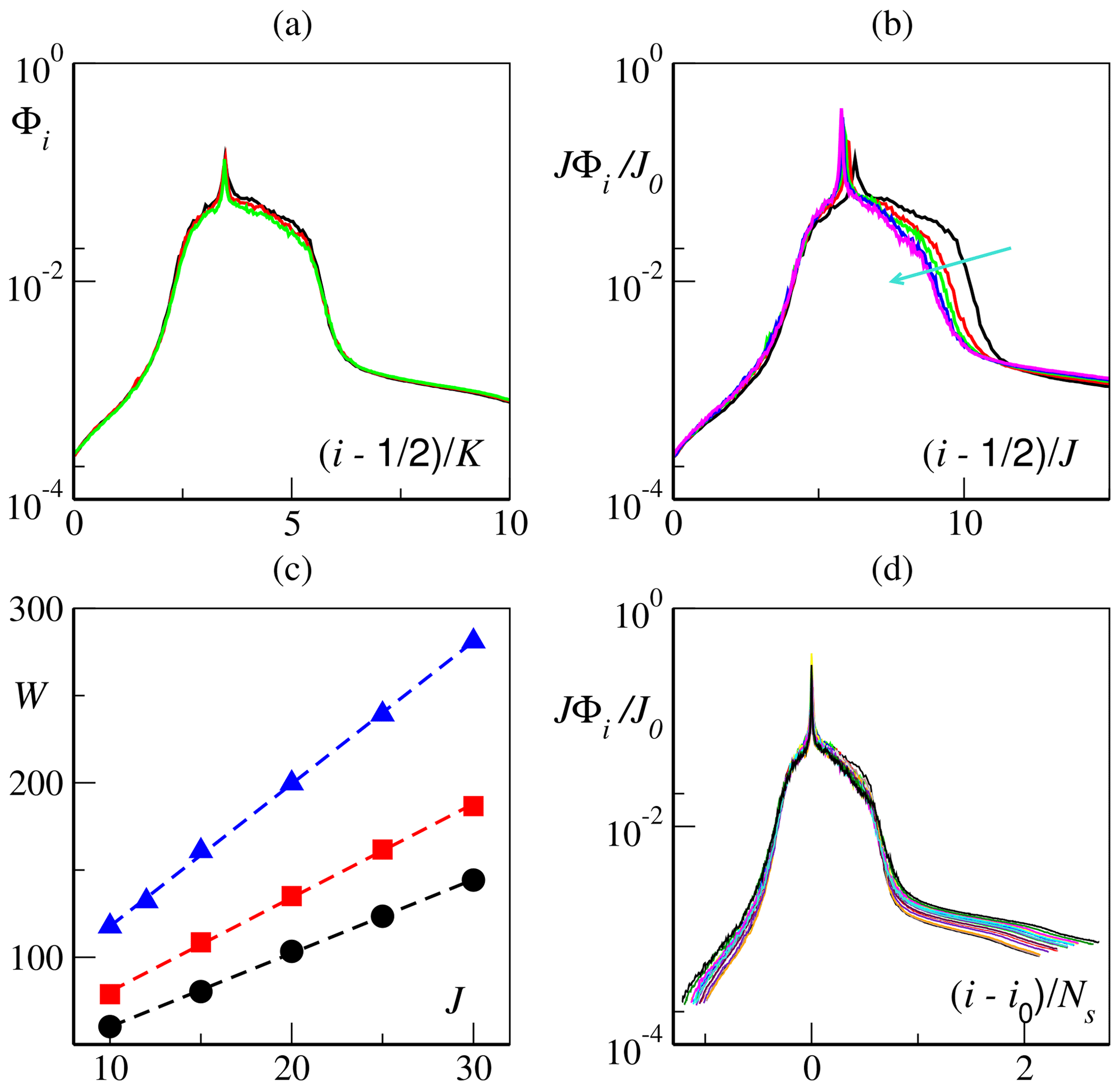
Figure 4 Slow-bundle scaling for h=0.5 and f=1. (a) CLV time-averaged X-projected norm Φ_i for K=18, 24 and 36 and J=10 vs. the rescaled index $(i-\mathrm{0.5})/K$. (b) Rescaled (see main text) CLV average projection norm Φ_i for K=18 and J=10, 15, 20, 25 and 30 (increasing along the cyan arrow) vs. the rescaled index $(i-\mathrm{0.5})/J$. A lack of precise collapse can be appreciated on the rightmost side of the central band. (c) Central band width W (see main text for details) as a function of J for K=18 (black circles), K=24 (red squares) and K=36 (blue triangles). The best linear fits, marked by the dashed lines, are $W=\mathrm{18}\left(\mathrm{1}\right)+\mathrm{4.20}\left(\mathrm{5}\right)J$ (for K=18), $W=\mathrm{26}\left(\mathrm{2}\right)+\mathrm{5.4}\left(\mathrm{1}\right)J$ (K=24) and $W=\mathrm{36}\left(\mathrm{2}\right)+\mathrm{8.2}\left(\mathrm{2}\right)J$ (K=36). (d) Rescaled CLV average projection norm Φ_i for K=18, 24 and 36 and J=10, 15, 20, 25 and 30 (all combinations) vs. the rescaled index $(i-i_{\mathrm{0}})/N_{\mathrm{s}}$. Here i₀ is the index of the 0-CLV and $N_{\mathrm{s}}=K(\mathrm{1}+\mathit{\alpha }J)$, with α≈0.22 (see text). We choose the vertical axis rescaling reference as J₀=10.

We next focus on the scaling with J at a fixed K. For the sake of computational simplicity, we first consider that K=18. As for the horizontal variable, it is natural to rescale the CLV index by the number J of fast degrees of freedom per subgroup. Moreover, since J corresponds to the ratio between the number of fast (K J) and slow (K) variables and we use the standard Euclidean norm to quantify the projection onto the X subspace, one expects the fraction Φ_i of the X norm to be inversely proportional to J. The projection data reported in Fig. 4b indeed show a convincing vertical collapse of the rescaled X norm Φ_iJ∕J₀ (here we fix a reference J₀=10), but accompanied by a shrinking of the central band on the right side, as J is increased.

In order to accurately determine the width of the central band, i.e., the slow-bundle dimension, we fix a threshold for the rescaled X norm, $J{\mathrm{\Phi }}_i/J_{\mathrm{0}}={\mathrm{10}}^{-\mathrm{2}}$ and estimate the number N_s of CLVs with a projection above such a threshold (we have verified that our results hold within a reasonable range of thresholds). The resulting widths N_s(K,J), computed for different numbers of slow variables K, are summarized in Fig. 4c, where they are plotted versus J. For the fixed K, we see a clear linear increase, compatible with the law

$$\begin{array}{}\text{(23)}& N_{\mathrm{s}}(K,J)=K\left(\mathrm{1}+\mathit{\alpha }J\right),\end{array}$$

where the coefficient α depends on the values of h, c, F_s and F_f. In the present case, a best fit gives α≈0.22. The most general representation of the projections is finally obtained by rescaling the index according to N_s and by using the 0-CLV (which corresponds to the peak of Φ_i) as the origin of the horizontal axis. The excellent collapse in Fig. 4d confirms the extensivity of the slow bundle with both K and J. The slow bundle is not a simple representation of the X subspace: it does not coincide with the slow variables themselves but involves also a finite fraction α of the fast ones, singling out a fundamental set of tangent-space perturbations closely associated with the slow dynamics. The origin of the phenomenological scaling law (23) will be discussed in the next section.

Before concluding this section, we would like to briefly discuss the time-resolved projected norm ϕ_i(t). So far, we have discussed time-averaged quantities, but it is worth mentioning that the X projections of individual CLVs are extremely intermittent, hinting at a complex tangent-space flow structure.

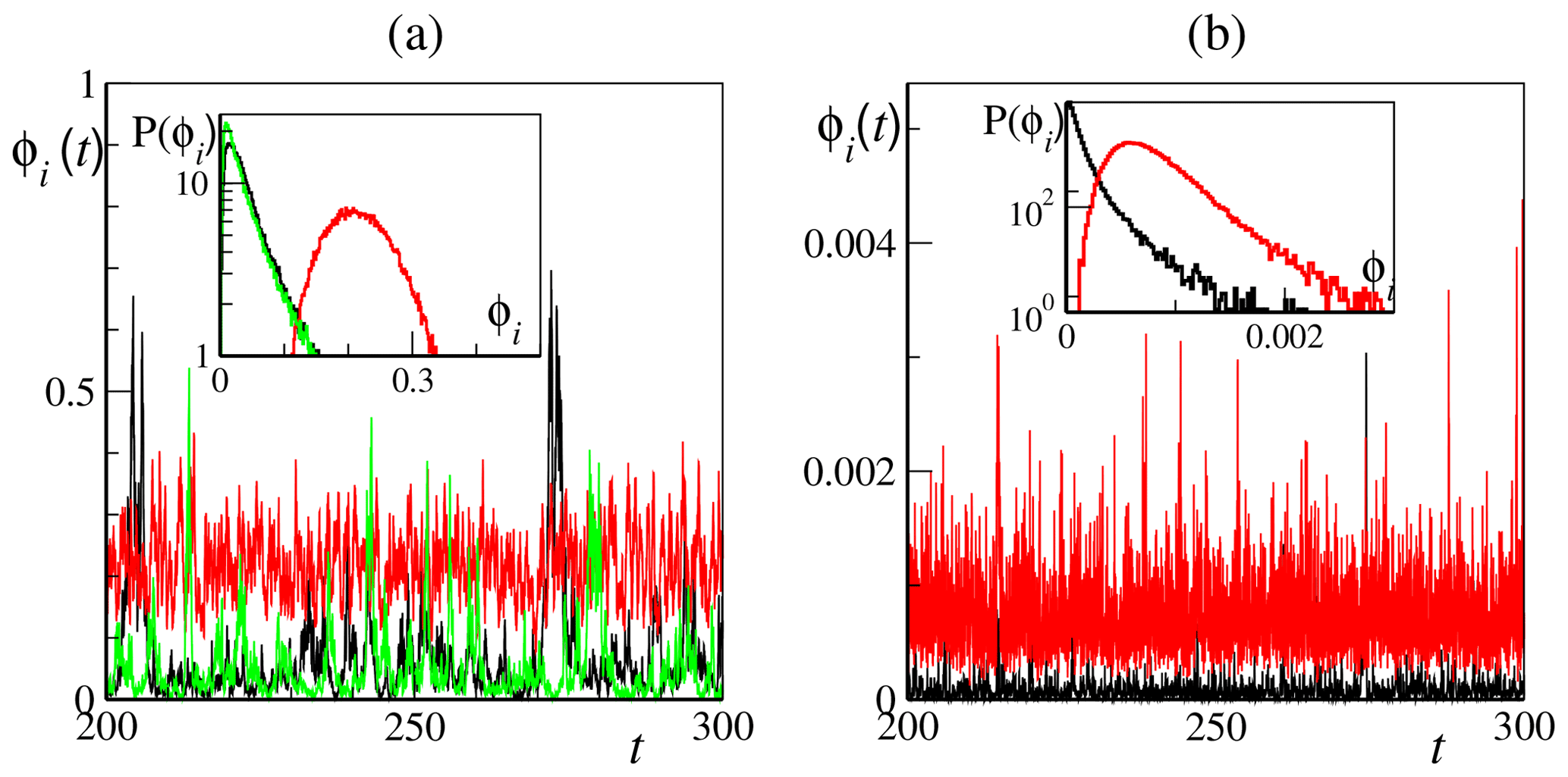
Figure 5 Time trace and probability distribution of CLV instantaneous projection in the X subspace for $h=\mathrm{1}/\mathrm{4}$ and b=10 and K=36 and J=10. (a) Slow-bundle vectors, i=110 (black line), i=122 (red line, the 0-CLV) and i=160 (green line). In the inset are the corresponding probability distributions of the three CLV time traces. (b) For two other CLVs with negligible X projection, first vector (black line) and 255th vector (red line). In the inset are corresponding probability distributions of the two CLV time traces.

In Fig. 5a we display a few selected time series of the norm ϕ_i(t) for b=10, K=36, J=10 and $h=\mathrm{1}/\mathrm{4}$ (the overall picture does not change qualitatively for different choices of the coupling strength). The time series correspond to the 110th vector, located in the left part of the central band (before the 0-CLV), the 160th vector, located in the right part, and the 0-CLV (vector index i=122). We clearly see a strong intermittency, resulting in a very skewed distribution of the time-resolved X norms. The 0-CLV is an exception, displaying more regular oscillations and a rather symmetric distribution around its mean value. This confirms the peculiar nature of the 0-CLV, whose delocalized structure is essentially determined by its alignment with the phase-space flow.

In Fig. 5b we display vectors outside the slow bundle: the 1st and the 250th, which are on the left- and right-hand side of the central band, respectively. We see that also vectors outside the slow bundle display a certain degree of intermittency, albeit on a faster timescale, and rather skewed distributions of their ϕ_i(t) values. Their X projection, of course, is strongly suppressed and remains very close to 0. In Sect. 4, we will further comment on the intermittent behavior of ϕ_i(t), showing that it arises from near degeneracies in the instantaneous instability rates.

4 The origin of the slow bundle

In the previous section, we have identified a slow bundle in the tangent space of the L96 model – a central band centered around the 0-CLV – whose covariant vectors are characterized by a large projection over the slow degrees of freedom. It is natural to expect this band to be associated not only with long timescales (i.e., the inverse of the corresponding LEs) but also with large-scale instabilities.

We begin by discussing the pedagogical example of the uncoupled limit (h=0). In this case, the X and Y subsystems evolve, by definition, independently, and one can separately determine K LEs associated with the slow variables and KJ exponents associated with the fast variables. The full spectrum can be thereby reconstructed by combining the two distinct spectra into a single one. The result is illustrated in Fig. 6a, where the red crosses correspond to the X LEs. Note that the same area is also spanned by the central part of the fast-variable spectrum. The region covered by the slow LEs, where the instability rates of the two uncoupled systems have the same magnitude, roughly corresponds to the location of the slow bundle in the coupled-model CLVs spectrum. This suggests that the origin of the slow bundle can be traced back to a sort of resonance between the slow variables and a suitable subset of the fast ones.

Note also that, in the absence of coupling, the Jacobian matrix has a block diagonal structure, with the CLVs either belonging to the X or Y subspaces. The projection Φ_i, therefore, is strictly equal to either 0 or 1, depending on the vector type, and can be used to distinguish the two types of vectors when the full set of (uncoupled) equations is integrated simultaneously.

We now proceed to discuss the coupled case. When the coupling is switched on, it has a double effect: (i) it modifies the overall dynamics, i.e., the evolution in phase space, in Eqs. (1a) and (1b), and (ii) it directly affects the tangent-space evolution, in Eqs. (18a) and (18b), destroying the block diagonal structure of the uncoupled Jacobian matrix. This, in turn, prevents one from identifying single LEs with either the slow or the fast dynamics. In order to be able to also distinguish the two contributions in the h>0 case, we study an intermediate setup characterized by a full coupling in real space but remove it from the tangent-space dynamics. In practice, we simulate the full nonlinear model (1a and 1b) and use the resulting trajectories to “force” an uncoupled tangent-space dynamics, that is

$$\begin{array}{ll}{\displaystyle }\mathit{\delta }{\dot{X}}_k& {\displaystyle }=\mathit{\delta }{X}_{k-\mathrm{1}}(X_{k+\mathrm{1}}-X_{k-\mathrm{2}})\\ \text{(24a)}& {\displaystyle }& {\displaystyle }+X_{k-\mathrm{1}}(\mathit{\delta }{X}_{k+\mathrm{1}}-\mathit{\delta }{X}_{k-\mathrm{2}})-\mathit{\delta }{X}_k,{\displaystyle }\mathit{\delta }{\dot{Y}}_{k,j}& {\displaystyle }=cb\left[\mathit{\delta }{Y}_{k,j+\mathrm{1}}\right(Y_{k,j-\mathrm{1}}-Y_{k,j+\mathrm{2}})\\ \text{(24b)}& {\displaystyle }& {\displaystyle }+Y_{k,j+\mathrm{1}}(\mathit{\delta }{Y}_{k,j-\mathrm{1}}-\mathit{\delta }{Y}_{k,j+\mathrm{2}})]-c\mathit{\delta }{Y}_{k,j},\end{array}$$

where the coupling terms, proportional to h in Eqs. (18a) and (18b), have been ignored. This way, the Jacobian matrix is still block diagonal.

Figure 6 (a) Lyapunov spectra for the uncoupled (h=0) case decomposed in its slow (λ^X; red crosses) and fast (λ^Y; black solid line) parts. (b) Full Lyapunov spectra (full lines) superimposed with spectra reconstructed from their restricted (see text) counterparts (dashed lines) for h=1 and $h=\mathrm{1}/\mathrm{16}$. (c) Root-mean-squared difference between the finite h restricted spectra and the completely uncoupled fast and slow spectra, for both fast (black squares) and slow (red circles) dynamics. Power law fits (dashed lines) return slopes close to unity (respectively ≈0.9 and ≈1.1), suggesting a simple linear growth with the coupling h. Blue diamonds refer to the root-mean-square difference Δλ^R between the full LS and the reconstructed ones in the restricted tangent-space approximation. Both axes are represented in a double logarithmic scale. In the upper part of (d) is an enlarged view of the central part ($i\in [\mathrm{50},\mathrm{250}]$ of the restricted spectra for $h=\mathrm{1}/\mathrm{8}$, with the slow (λ^X, red crosses) and fast (λ^Y, black solid line) components differently marked. In the lower part of the panel is the same enlarged view of the $h=\mathrm{1}/\mathrm{8}$ projection norm, as computed from the fully coupled dynamics. The vertical red dashed lines mark the upper (i_L) and lower (i_R) boundaries of the superposition region as reported in Table 1. In all panels, we have fixed the following: b=10, K=36 and J=10.

Thanks to this approximation, we can define two restricted spectra ${\mathit{\lambda }}_k^X$ and ${\mathit{\lambda }}_j^Y$ for the slow and fast variables, respectively, and thereby recombine them into a single spectrum by ordering the exponents from the largest to the most negative one. A comparison between the resulting reconstructed spectra and the full ones (with coupling acting both in real and tangent space) shows an excellent agreement, at least in the range $h\in (\mathrm{0},\mathrm{1})$. Two examples for h=1 and $h=\mathrm{1}/\mathrm{16}$ are given in Fig. 6b, while the dependence of their root-mean-square difference Δλ^R on h is reported in Fig. 6c (blue diamonds). It is not, however, clear to what extent this is a general property of high-dimensional dynamics; we are not aware of similar analyses made in high-dimensional models.

The modifications induced by real-space coupling are more substantial. They can be quantified by computing the root-mean-square differences

$$\begin{array}{ll}\text{(25)}& {\displaystyle }\mathrm{\Delta }{\mathit{\lambda }}^X\left(h\right)& {\displaystyle }=\sqrt{{\displaystyle \frac{\mathrm{1}}{K}}\sum _{k=\mathrm{1}}^K{\left[{\mathit{\lambda }}_k^X\left(h\right)-{\mathit{\lambda }}_k^X\left(\mathrm{0}\right)\right]}^{\mathrm{2}}},{\displaystyle }\mathrm{\Delta }{\mathit{\lambda }}^Y\left(h\right)& {\displaystyle }=\sqrt{{\displaystyle \frac{\mathrm{1}}{KJ}}\sum _{j=\mathrm{1}}^{KJ}{\left[{\mathit{\lambda }}_j^Y\left(h\right)-{\mathit{\lambda }}_j^Y\left(\mathrm{0}\right)\right]}^{\mathrm{2}}},\end{array}$$

which measure the average variation in the restricted spectra upon increasing the coupling. Numerical simulations, reported in Fig. 6c, show that both Δλ^X and Δλ^Y increase approximately linearly with h, the main difference being that ${\mathit{\lambda }}_k^X\left(h\right)$ values decrease (in absolute value) when h is increased, while the opposite holds for ${\mathit{\lambda }}_j^Y\left(h\right)$. In Fig. 6c, we can also appreciate that both Δλ^X and Δλ^Y are significantly larger than Δλ^R, showing that tangent-space coupling is not relevant for the estimate of the LEs. On the other hand, this is not expected to be true for the CLVs, which are local objects, defined at each attractor point. CLVs associated with the restricted LEs are, by definition, confined either to the X or the Y subspace so that their X projection Φ_i is again either equal to 0 or 1. The analysis carried out in the previous section for the fully coupled dynamics shows instead that the average projection Φ_i of any vector within the slow bundle is significantly different from both 0 and 1 and substantially constant over the entire central band. This means that the orientation of the CLVs is very sensitive to the coupling itself.

The main mechanism responsible for the reshuffling of the CLV orientation is the (multifractal) fluctuations of finite-time LEs (Pikovsky and Politi, 2016). Fluctuations are the unavoidable consequence of the different degrees of stability experienced in different regions of the phase space, and they occur in both strictly hyperbolic and nonhyperbolic dynamical systems, although they are typically much larger in the latter context. Fluctuations may be so large as to bridge the gap between distinct LEs, which results in a lack of domination of the Oseledets splitting (Pugh et al., 2004; Bochi and Viana, 2005) and in the sporadic occurrence of near tangencies between pairs of different CLVs (Yang et al., 2009; Takeushi et al., 2011)⁵. Fluctuations are also responsible for the so-called coupling sensitivity (Daido, 1984; Pikovsky and Politi, 2016): strictly degenerate LEs in uncoupled systems may separate by an amount of the order of $\mathrm{1}/\left|\ln \mathit{\epsilon }\right|$, where ε is the (small) amplitude of the coupling strength.

Let us be more quantitative and introduce the finite-time Lyapunov exponents γ_i(t), computed from the average expansion rate over a window of length τ_w,

$$\begin{array}{}\text{(26)}& {\mathit{\gamma }}_i\left(t\right)={\displaystyle \frac{\mathrm{1}}{{\mathit{\tau }}_{\mathrm{w}}}}\ln \left|\right|\mathbf{M}({\mathit{x}}_t,{\mathit{\tau }}_{\mathrm{w}}){\mathit{v}}_i\left(t\right)\left|\right|,\end{array}$$

where M(x_t,τ_w) is the propagator (15) for the tangent-space evolution over time τ_w, while the CLVs v_i is normalized to unity. Their asymptotic time average obviously coincides with the corresponding LEs, 〈γ_i(t)〉_t≡λ_i.

We are interested in the probability distribution P(γ_i) of γ_i, obtained by evolving a long trajectory. For short times, γ_i fluctuations significantly depend on the coordinates used to parametrize the dynamics, but upon increasing τ_w, such a variability is progressively lost and the width of P(γ) scales as $\mathrm{1}/\sqrt{{\mathit{\tau }}_{\mathrm{w}}}$, as prescribed by the multifractal formalism (Pikovsky and Politi, 2016). In the following, we have set τ_w=0.5, after having verified that it is long enough. Here, for illustrative purposes, we have selected two vectors which, in the absence of tangent-space coupling, are of the X and Y type, respectively⁶. From Fig. 7a, it is clear that the amplitude of the fluctuations largely exceeds the difference between the corresponding mean values (i.e., the asymptotic LEs; see the vertical straight lines) and that the same holds true after restoring the coupling in tangent space (Fig. 7b).

Consistently, in Fig. 7c, we show that the corresponding CLVs are characterized by nonnegligible near tangencies: The probability distribution of the relative angle,

$$\begin{array}{}\text{(27)}& {\mathit{\theta }}_{i,j}\left(t\right)=\arccos \left[{\mathbf{v}}_i\left(t\right)\cdot {\mathit{v}}_j\left(t\right)\right],\end{array}$$

indeed exhibits a peak near 0.

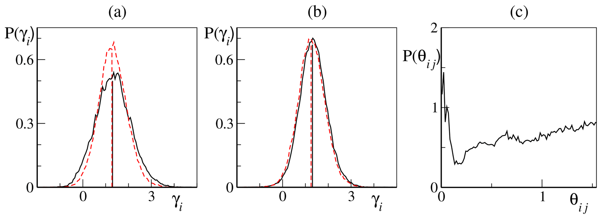
Figure 7 (a–b) Probability distribution of the finite-time LEs (26) for two nearby LEs belonging to the slow bundle. We show results for the 92nd (black solid line) and 93rd (red dashed line) LEs which, in the absence of tangent-space coupling (the restricted setup; see text), belong, respectively, to the λ^X and λ^Y restricted spectra. (a) Finite-time LEs fluctuations in the restricted case. The vertical lines mark the mean values ${\mathit{\lambda }}_{\mathrm{92}}^X=\mathrm{1.30}$ and ${\mathit{\lambda }}_{\mathrm{93}}^Y=\mathrm{1.275}$ (indices refer to the full spectrum position, and they correspond to the 5th and 88th, respectively, LE in the X and Y restricted spectra). (b) Finite-time LEs fluctuations in the fully coupled case. The vertical lines mark the mean values λ₉₂=1.31 and λ₉₃=1.25. (c) Probability distribution of the angle θ_ij (see Eq. 27) between the two corresponding CLVs in the fully coupled case. All simulations have been performed for K=36, J=10, b=10 and $h=\mathrm{1}/\mathrm{16}$. We have fixed the following in all panels: K=36 and J=10.

We have verified this to be the generic behavior, as expected due to the nonhyperbolic nature of the L96 model. The near tangencies between different CLVs within the slow bundle provide strong numerical evidence of the mixing between slow and fast degrees of freedom and are perfectly consistent with the nonnegligible projection onto the slow X subspaces of all vectors in the slow bundle. In fact, in the presence of two similarly unstable directions, the corresponding CLVs tend to wander in a (fluctuating) two-dimensional subspace, selecting their current direction on the basis of the relative degree of instability. It is therefore natural to expect that, in the presence of strong fluctuations, an X-type vector (in the uncoupled limit) temporarily aligns along the Y directions and vice versa, thereby giving rise to a projection pattern such as the one seen in the central region of the CLVs spectrum, where all vectors have a nonnegligible average projection over the X degrees of freedom.

The intermittent nature of the instantaneous X projection ϕ_i(t) discussed in Sect. 3.1 further validates this picture: it is the result of the large fluctuations exhibited by finite-time LEs, which are, in turn, associated with changes of directions when the CLV comes close to tangencies. Furthermore, the large ratio between the amplitude of the fluctuations and the separation between consecutive LEs suggests that this exchange of directions may extend beyond the nearest neighbors along the spectrum. We conjecture that the relatively smooth boundary of the central band is precisely a manifestation of this sort of extended interaction.

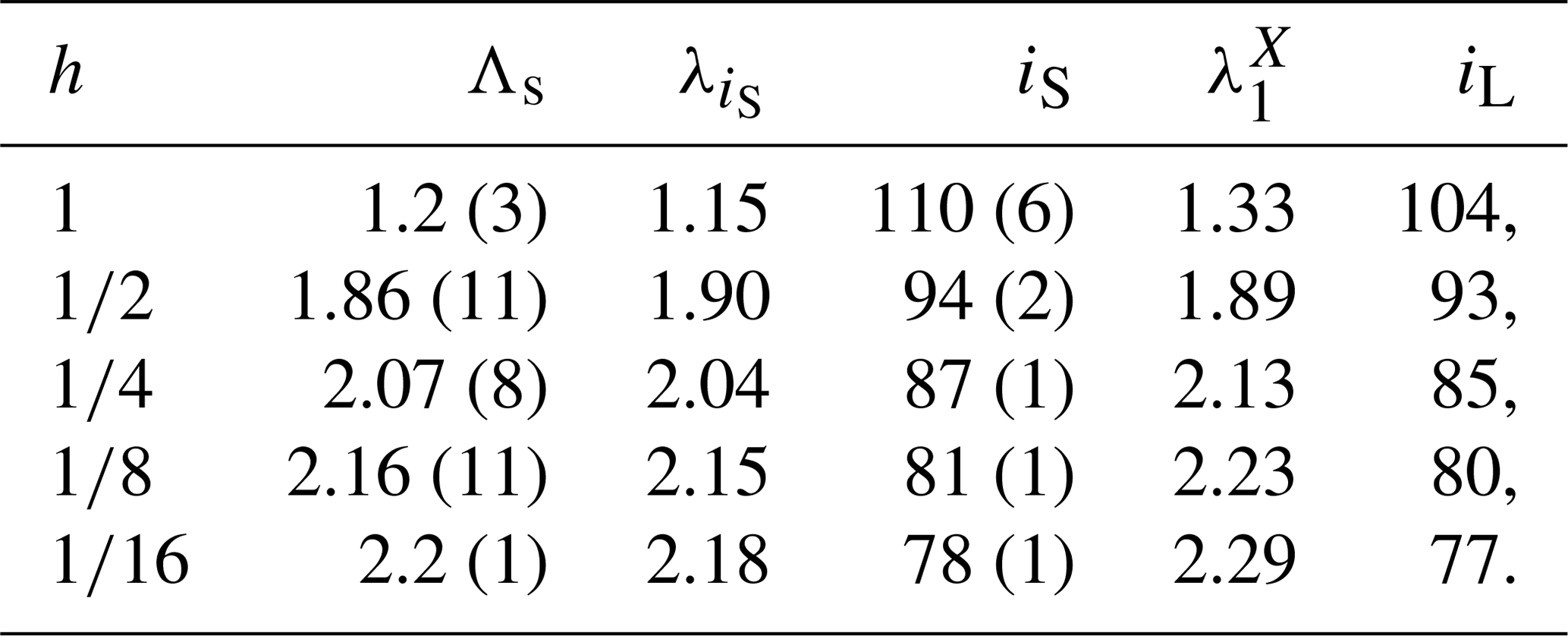
Finally, we return to the restricted LEs to see whether – as implied by the above conjecture – their knowledge can help to identify the slow-bundle boundaries. In practice, we have first identified the borders of the region covered by both slow LEs. They are given by the indices (within the reconstructed spectrum) of the largest and smallest restricted slow LE, labeled, respectively, as i_L and i_R. They are reported in Table 1, together with the corresponding value of the restricted Lyapunov exponent, for different coupling values. The agreement with the actual boundaries of the slow bundle – as revealed by a visual inspection of the projection patterns Φ_i – is actually pretty good (see, e.g., Fig. 6d for $h=\mathrm{1}/\mathrm{8}$).

Table 1 X-restricted largest (${\mathit{\lambda }}_{\mathrm{1}}^X$) and smallest (${\mathit{\lambda }}_K^X$) LE with the corresponding full spectrum indices (i_L and i_R). All data refer to b=10, K=36 and J=10.

Altogether, our analysis suggests that coupling in real space induces a sort of “short-range” interaction within tangent space: each LE (and the corresponding CLV) tends to affect and be affected by exponents with a similar magnitude and thereby characterizes a similar degree of instability in a sort of resonance phenomenon.

Note finally that the spectral band where the slow and fast restricted Lyapunov spectra superimpose covers all the slow restricted LEs and a finite fraction of the fast ones, thus providing a justification of the phenomenological scaling law (23).

5 Finite perturbations

So far we have studied the geometry of the L96 model, dealing exclusively with infinitesimal perturbations. A legitimate question is whether we can learn something more by looking at finite perturbations.

Finite-size analysis has been implemented in the L96 model since its introduction (Lorenz, 1996), and it has been formalized with the definition of the so-called finite-size Lyapunov exponents (FSLEs; Aurell et al., 1997). In a nutshell, the rationale for introducing FSLEs is – as already recognized by Lorenz – that in nonlinear systems the response to finite perturbations may strongly depend on the observation scale. Dropping the limit of vanishing perturbations, of course, weakens the level of mathematical rigor of the infinitesimal Lyapunov analysis, but it nevertheless allows for a meaningful study of the underlying instabilities.

Here, we follow the excellent review (Cencini and Vulpiani, 2013), where applications to L96 were also discussed. Given a generic trajectory x(t), the idea is to define a series of thresholds δ_n=δ₀σⁿ, with σ>1, and to measure the times τ(δ_n) needed by the norm of a finite perturbation $\mathrm{\Delta }\mathit{x}\left(t\right)={\mathit{x}}^{\prime }\left(t\right)-\mathit{x}\left(t\right)$ to grow from the amplitude δ_n to δ_n+1. The FSLE Λ(δ_n) is then defined as

$$\begin{array}{}\text{(28)}& \mathrm{\Lambda }\left({\mathit{\delta }}_n\right)={\displaystyle \frac{\ln \mathit{\sigma }}{\langle \mathit{\tau }\left({\mathit{\delta }}_n\right)\rangle }},\end{array}$$

where 〈⋅〉 denotes an average over many realizations of the perturbation. In practice, one starts at time t₀ with a finite perturbation ∥Δx(t₀)∥≪δ₀ to ensure a correct alignment (along the most expanding direction) by the time the perturbation amplitude reaches the first threshold δ₀. Subsequently, both trajectories x and x^′ are followed, registering the crossing times of all δ_n thresholds. By repeating this procedure many times, one is able to estimate the FSLEs for all amplitudes δ_n via Eq. (28). The FSLE in principle depends on the norm used to define the size of the perturbation (Cencini and Vulpiani, 2013). However, by construction, for vanishing perturbations, the FSLE should coincide with the largest LE, regardless of the norm:

$$\begin{array}{}\text{(29)}& \underset{\mathit{\delta }\to \mathrm{0}}{lim}\mathrm{\Lambda }\left(\mathit{\delta }\right)={\mathit{\lambda }}_{\mathrm{1}}.\end{array}$$

In Cencini and Vulpiani (2013), FSLEs have been applied to analyze the L96 model (see also Boffetta et al., 1998, for an earlier study). In a slightly different setup (no fast-variable forcing and a larger scale separation b), it was shown that the FSLE is characterized by two different plateaus: (i) a small-δ one, essentially associated with the instability of the fast, convective degrees of freedom and roughly equivalent to the largest LE, Λ(δ)≈λ₁, and (ii) a large-δ plateau that was associated with the intrinsic instability Λ_s on the slow larger scales. Interestingly, it was observed that also the height of the second plateau seems to be roughly norm independent. This observation led to the conjecture that the nonlinear evolution of large perturbations may be controlled by the linear dynamics of an effective lower-dimensional system, capturing the essence of the slow-variable dynamics (Cencini and Vulpiani, 2013).

In this section we repeat this analysis in our setup, comparing the behavior of the FSLE with the analysis of the tangent-space slow bundle. In the following we use our standard parameters (K=36, J=10 and b=10), using $\mathit{\sigma }=\sqrt{\mathrm{2}}$ and ${\mathit{\delta }}_{\mathrm{0}}={\mathrm{10}}^{-\mathrm{3}}$ and averaging the crossing times over 10³ realizations. For each realization, the initial finite perturbation $(\mathrm{\Delta }{X}_{\mathrm{1}},\mathrm{\dots },\mathrm{\Delta }{X}_K,\mathrm{\Delta }{Y}_{\mathrm{1},\mathrm{1}},\mathrm{\Delta }{Y}_{K,J})$ is chosen at random, with an initial amplitude of 10⁻⁵.

As we expect the FSLE to depend on the norm, we have decided to transform this weakness into an advantage by studying the behavior of an entire family of Euclidean norms, thereby extracting useful information from the dependence on the chosen norm. More precisely, we introduce the γ-dependent norm

$$\begin{array}{}\text{(30)}& {∥\cdot ∥}_{\mathit{\gamma }}=\sqrt{\sum _k{X}_k^{\mathrm{2}}+\mathit{\gamma }\sum _{k,j}{Y}_{k,j}^{\mathrm{2}}},\end{array}$$

which, for γ=1, coincides with the standard Euclidean norm. We consider $\mathit{\gamma }\in (\mathrm{0},\mathrm{1}]$, a choice which allows exploring a broad range of weights of the slow variables.

Figure 8 FSLE analysis. (a) FSLEs for different coupling constants, h=1 (black line), $h=\mathrm{1}/\mathrm{2}$ (red line), $h=\mathrm{1}/\mathrm{4}$ (green line), $h=\mathrm{1}/\mathrm{8}$ (blue line) and $h=\mathrm{1}/\mathrm{16}$ (red line) – decreasing along the cyan arrow – vs. the finite-size amplitudes δ_n for the $\mathit{\gamma }={\mathrm{10}}^{-\mathrm{3}}$ norm. In the inset are the FSLEs for $h=\mathrm{1}/\mathrm{4}$ and different γ norms (γ=1, 10⁻¹, 10⁻² and 10⁻³, decreasing along the orange arrow). The error bars measure one standard error. The black dashed line marks the FSLEs for the limiting case γ→0. Note the logarithmic scale for the abscissa of both graphs. (b) Details of the LE spectrum (top part of panel) and of the Φ_i average projection norm patterns (bottom part of panel) as in Fig. 3b. The solid dots and the vertical dashed line mark the value and the location of the LEs ${\mathit{\lambda }}_{i_{\mathrm{S}}}$ as identified in Table 2 (see main text for more details). Different coupling constant values are color-coded as in panel (a), with h decreasing along the cyan arrow in the top part of the panel.

In the inset of Fig. 8a, we see that the main effect of changing the norm is a variation in the length of the two plateaus: upon decreasing γ, the first plateau shrinks, leaving space for a longer second plateau. The height of the two plateaus is largely γ independent. This behavior can be qualitatively understood as follows. At early times, all components of the perturbation grow according to the maximum LE, which we know from the previous analysis to be mostly controlled by the dynamics of the fast Y variables. As time goes on, the perturbations of the Y variables start saturating, while those of the slow variables keep growing, however, at a pace controlled by their (weaker) intrinsic instability. Upon decreasing γ, the relative weight of the less unstable, slow variables increases. However, there is a limit: even when γ→0, the growth rate of the X perturbations is initially controlled by the fast variable. The range of this initial, approximately linear regime depends on the initial amplitude of the fast components; this limit corresponds to the dashed curve in the inset of Fig. 8a.

The FSLEs obtained for different coupling parameters h are shown in Fig. 8a, all for $\mathit{\gamma }={\mathrm{10}}^{-\mathrm{3}}$. Two plateaus are clearly visible, at least for h<1. The first one coincides with the maximum LE of the whole system, as per Eq. (29). The second one approximately extends over a range of 1 order of magnitude (at large scales, the plateau is obviously limited by the attractor size). Its height corresponds to the characteristic instability Λ_s(h) associated with the effective dynamics of the slow variables, as conjectured in Cencini and Vulpiani (2013).

For each coupling h, we estimated the corresponding Λ_s(h) as the average of Λ(δ_n) in the interval ${\mathit{\delta }}_n\in [\mathrm{1},\mathrm{10}]$ and identified the closest LE ${\mathit{\lambda }}_{i_{\mathrm{S}}}$ and its index i_S in the Lyapunov spectra. The results of this procedure are summarized in Table 2 and compared with the results of the restricted analysis obtained in Sect. 4.

Table 2 Estimated slow dynamics finite-size instability Λ_s(h) compared to the closest LE and its index i_S for different coupling constants. Numbers in parenthesis refer to the uncertainty in Λ_S and, accordingly, of i_S. Results of the restricted analysis carried on in Sect. 4 are reported from Table 1 for comparison. All data have been obtained with b=10, K=36 and J=10.

In practice, by interpreting the height of each plateau as a suitable instability rate within the full Lyapunov spectrum, one can thereby extract the corresponding index i_S for each value of the coupling constant. In Fig. 8b we have marked these indices with dashed vertical lines (upper part of panel) and compared with the slow-bundle projection patterns (lower part of panel). Interestingly, these values seem to provide a reasonable estimate of the leftmost boundary of the central band which defines the slow bundle in tangent space. Essentially, i_s coincides fairly well with the left “shoulder”, where Φ_i starts to drop towards negligible values for decreasing i. Note, however, that for larger values of h, the second plateau becomes less sharply defined, up to the case h=1, where it is practically impossible to define a threshold. Correspondingly, the boundaries of the slow bundle in tangent space, as defined by inspection of Φ_i, also become less well defined.

Altogether, the slow-variable (large-scale) instability Λ_s emerging from the finite-size analysis roughly coincides with the upper boundary of the slow bundle (i.e., the LEs associated with the CLVs with a relevant projection onto the X_k variables). Following the analysis of the restricted spectra carried out in the previous section, Λ_s is also close to the first restricted LE associated with the X subspace ${\mathit{\lambda }}_{\mathrm{1}}^X$, as shown in Table 2. The parameter γ proves to be useful in improving the accuracy of the two plateaus exhibited by the FSLEs.

It is remarkable that the analysis of a single pair of trajectories allows for extracting information about (at least) two different Lyapunov exponents. We conjecture that the linearly controlled growth of small, finite perturbations stops as soon as the fast components saturate because of nonlinearities. Afterwards, fast variables act as a sort of noise on the slow ones, whose dynamics is still in the linear regime. Finally, in view of the above-mentioned closeness between the restricted and fully coupled LS, it is reasonable to conjecture that, since coupling does not play a crucial role in tangent space, the growth rate corresponds, in this second regime, to the maximal LE of the slow variables, as indeed observed. Our result supports an earlier conjecture of Cencini and Vulpiani (2013) concerning the existence of an effective lower-dimensional dynamics capturing the slow-variable behavior.

6 Discussion and conclusions

Our analysis of the tangent-space structure of the L96 model has identified a slow bundle within the full tangent space. It is composed of the set of covariant Lyapunov vectors characterized by a nonnegligible projection over the slow degrees of freedom. Vectors in this set are associated with the smallest (in absolute value) LEs and thus with the longest timescales. We have verified that the number of such vectors increases linearly with the total number of degrees of freedom so that the slow-bundle dimension is an extensive quantity.

The upper and lower boundaries of the slow bundle are better defined for a weak coupling h. However, the rescaled formulation of L96 (see Eq. 4a) shows that the effective upward coupling (from the fast to the slow variables) is $hf=hJc/b^{\mathrm{2}}$, thereby suggesting that an increase of the amplitude separation b can increase the sharpness of the slow-bundle boundaries even for large h. As reported in Fig. 9a, numerical simulations with h=1 and increasing values of b actually confirm this intuition, indicating that a slow bundle can be clearly defined also in the strong coupling limit, provided that the slow- and fast-scale amplitudes are sufficiently separated.

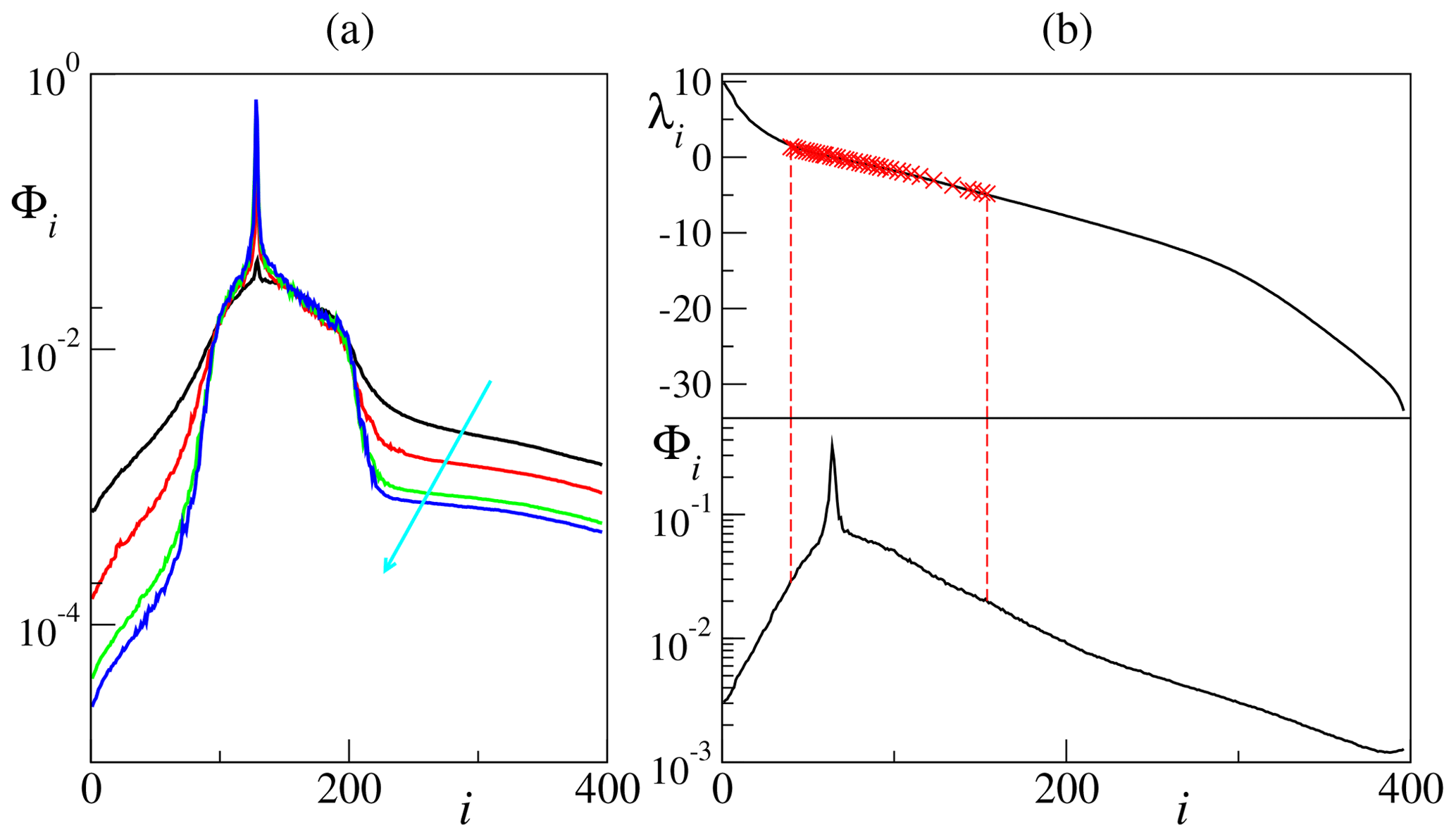
Figure 9 (a) X-projection patterns Φ_i for Lorenz 96 with fast-variable forcing (F_f=6), strong coupling h=1 and increasing (along the direction of the cyan arrow) values of amplitude separation, b=10, 20, 40 and 50. (b) Lyapunov spectrum (top part of panel) and X-projection patterns (bottom part of panel) for Lorenz 96 with no fast-variable forcing (F_f=0) and standard parameter values, h=1 and $b=c=\mathrm{10}$. The red crosses mark the values of the X-restricted spectrum (see Sect. 4 for more details). System size is K=36 and J=10 in both panels.

In order to clarify the origin of the slow bundle, we have introduced the notion of restricted Lyapunov spectra and argued that the central region, where the CLVs retain a significative projection over both slow and fast variables, corresponds to the range where the restricted spectra overlap with one another. In this region, fluctuations of the finite-time LEs much larger than the typical separation between consecutive LEs lead inevitably to frequent “near tangencies” between CLVs, thereby mixing slow and fast degrees of freedom into a nontrivial set of vectors which carries information on both sets of variables.

Besides, we have found that coupling in tangent space weakly influences the actual LEs, provided that it is accounted for in real space. This is one of the reasons for the finite-size analysis being able to give information about the instability of the slow bundle (i.e., the correspondence between the second plateau displayed by the FSLE and the upper boundary of the slow bundle). Further investigations are necessary to put our consideration on firmer ground.

So far, we have discussed the slow bundle in a setup where the fast degrees of freedom are forced by a strong external drive F_f so that the fast dynamics is intrinsically chaotic even in the absence of coupling. One might wonder how general these results are and, in particular, how they could be extended to the traditional L96 setup, with no forcing of the fast variables (Lorenz, 1996). When F_f=0, in the zero-coupling limit, the fast dynamics is dominated by dissipation with no chaotic features. However, it is easy to verify that for a sufficiently strong coupling, the fluctuations of the slow variables induce a chaotic dynamics on the fast ones as well so that the “classical” setup resembles the forced one analyzed in this paper. While we have not performed an accurate and thorough study, preliminary simulations indicate that the signature of a slow bundle can be found also in the classical setup for sufficiently strong coupling. In particular, as reported in Fig. 9b for h=1, one can see that the region of nonnegligible X projections of the CLVs again coincides with the superposition region of the slow and fast restricted spectra.

As already mentioned, the slow bundle is identified as the set of CLVs with a nonnegligible projection onto the slow degrees of freedom. One might argue that the average projection Φ on the X subspace decreases with J, being at best of the order of 1∕J, i.e., the fraction of slow degrees of freedom. However, what matters is not the actual value of Φ but rather the ratio between the height of the plateau and that of the underlying background. The scaling analysis reported in Fig. 4 shows that this ratio stays finite while increasing the number of fast variables.

Altogether, we conjecture that (i) the fast stable directions lying beyond the slow-bundle central region are basically slaved degrees of freedom, which do not contribute to the overall dynamical complexity, and (ii) the fast unstable directions act as a noise generator for the Y degrees of freedom (their projection onto the X variables being negligible, and they do not talk directly with the slow variables). Therefore, it is natural to conjecture that the two subsystems mutually interact only through the slow-bundle instabilities so that suitably aligned perturbations of the fast variables can affect the slow variables and vice versa (see also Vannitsem and Lucarini, 2016). While this is a mere conjecture to be explored in future works, it suggests that (some) covariant vectors could be profitably applied to ensemble forecasting and data assimilation in weather and climate models. In particular, it has already been shown that restricting variational data assimilation to the full unstable subspace can increase the forecasting efficiency (Trevisan and Uboldi, 2004; Trevisan et al., 2010). In the future, we would like to explore whether a data assimilation scheme restricted to the slow bundle only (which does not encompass the entire unstable space) can lead to further improvements in forecasting.

The mechanism discussed in Sect. 4, relying on the overlap of the two restricted Lyapunov spectra should be common in nonlinear multiscale systems; therefore we believe our findings to be fairly generic. In the future, it will be interesting to extend the present analysis of Lyapunov exponents and covariant Lyapunov vectors to models with multiple scales and/or higher complexity and relevance, such as the coupled atmosphere–ocean model MAOOAM (De Cruz et al., 2016), or simplified multilayer models of the atmosphere, such as PUMA (Fraedrich et al., 2005) or SPEEDY (Molteni, 2003), thus going beyond the LEs studies of De Cruz et al. (2018) to include the full tangent-space geometry.