Denoising stacked autoencoders for transient electromagnetic signal denoising

The transient electromagnetic method (TEM) is extremely important in geophysics. However, the secondary field signal (SFS) in the TEM received by coil is easily disturbed by random noise, sensor noise and man-made noise, which results in the difficulty in detecting deep geological information. To reduce the noise interference and detect deep geological information, we apply autoencoders, which make up an unsupervised learning model in deep learning, on the basis of the analysis of the characteristics of the SFS to denoise the SFS. We introduce the SFSDSA (secondary field signal denoising stacked autoencoders) model based on deep neural networks of feature extraction and denoising. SFSDSA maps the signal points of the noise interference to the high-probability points with a clean signal as reference according to the deep characteristics of the signal, so as to realize the signal denoising and reduce noise interference. The method is validated by the measured data comparison, and the comparison results show that the noise reduction method can (i) effectively reduce the noise of the SFS in contrast with the Kalman, principal component analysis (PCA) and wavelet transform methods and (ii) strongly support the speculation of deeper underground features.

1 Introduction

Through the analysis of the secondary field signal (SFS) in the transient electromagnetic method (TEM), the information of underground geological composition can be obtained and has been widely used in mineral exploration, oil and gas exploration, and other fields (Danielsen et al., 2003; Haroon et al., 2014). Due to the small amplitude of the late field signal in the secondary field, it may be disturbed by random noise, sensor noise, human noise and other interference (Rasmussen et al., 2017), which leads to data singularities or interference points, and thus the deep geological information can not be reflected well. Therefore, it is necessary to make full use of the characteristics of the secondary field signal to reduce the noise in the data and increase the effective range of the data.

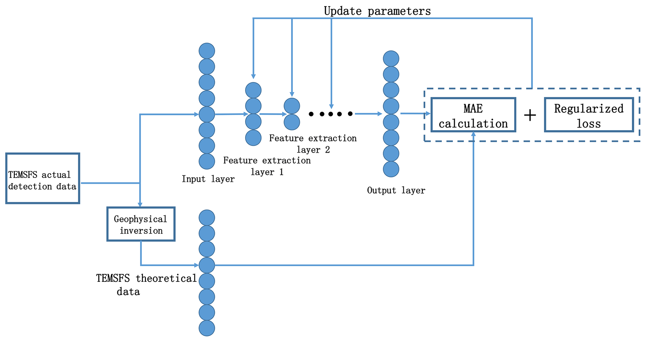
Figure 1 The flow chart of the model. Total loss is the sum of the mean absolute error (MAE) calculation and regularization loss. The MAE calculation is the difference of the theoretical signal and output. The regularization loss is calculated by the L2 function. Autoencoders (AEs) are trained one by one and then fine-tuning is used.

Figure 2 (a) Actual signal curves. (b) Inversion of theoretical signal curves.

Many methods have been developed for noise reduction of the transient electromagnetic method. These methods can be broadly categorized into three groups: (1) Kalman filter algorithm (Ji et al., 2018), (2) wavelet transform algorithm (Ji et al., 2016; Li et al., 2017) and (3) principal component analysis (PCA) (Wu et al., 2014). Kalman filtering is an effective method in linear systems, but it has little effect in nonlinear fields such as transient electromagnetic signals. The acquisition of the wavelet threshold is cumbersome, and wavelet base selection is very difficult. In order to achieve the desired separation effect, it is necessary to design an adaptive wavelet base. Likewise, the PCA algorithm is cumbersome too; some researchers applied PCA to denoise the transient electromagnetic signal, but the process of PCA requires at least five steps (Wu et al., 2014).

However, deep learning has been used to reduce noise from images, speech and even gravitational waves (Jifara et al., 2017; Grais et al., 2017; Shen et al., 2017). Meanwhile, the autoencoder (AE) (Bengio et al., 2007), the representative model of deep learning, has been successfully applied in many fields (Hwang et al., 2016). AEs with noise reduction capability (denoising autoencoders, DAEs) (Vincent et al., 2008) have been widely used in image denoising (Zhao et al., 2014), audio noise reduction (Dai et al., 2014), the reconstruction of holographic image denoising (Shimobaba et al., 2017) and other fields.

Nevertheless, in the field of geophysics, the application of the deep learning model is limited (Chen et al., 2014). The use of the deep learning model to reduce the noise of geophysical signals has not been applied. Therefore, in this paper, the SFSDSA (secondary field signal denoising stacked autoencoders) model is proposed to reduce noise, based on a deep neural network with SFS feature extraction. SFSDSA will map the signal points affected by noise to the high-probability points with geophysical inversion signal as reference according to the deep characteristics of the signal, so as to realize the signal denoising and reduce noise interference.

2 Related work

Many studies about the denoising of the second field signal of the transient electromagnetic method have been carried out. Ji et al. proposed a method using the wavelet threshold-exponential adaptive window width-fitting algorithm to denoise the second field signal (Ji et al., 2016). According to this method, stationary white noise and non-stationary electromagnetic noise can be filtered using the wavelet threshold-exponential adaptive window width-fitting algorithm to denoise the second field signal; Li et al. used the stationary-wavelet-based algorithm to denoise the electromagnetic noise in grounded electrical source airborne transient electromagnetic signal (Li et al., 2017). This denoising algorithm can remove the electromagnetic noise from the grounded electrical source airborne transient electromagnetic signal. Wang et al. used the wavelet-based baseline drift correction method for grounded electrical source airborne transient electromagnetic signals; it can improve the signal-to-noise ratio (Wang et al. 2013). An exponential fitting-adaptive Kalman filter was used to remove mixed electromagnetic noises (Ji et al., 2018). It consists of an exponential fitting procedure and an adaptive scalar Kalman filter. The adaptive scalar Kalman uses the exponential fitting results in the weighting coefficients calculation.

The aforementioned Kalman filter and wavelet transform are universal traditional filtering methods, which have their own defects. However, the SFS itself has distribution characteristics, and the distortion of the waveform generated by the noise causes deviation from the signal point of the distribution.

Theoretical research (Bengio et al., 2007) indicates that the incomplete representation of autoencoders will be forced to capture the most prominent features of the training data and the high-order feature of data is extracted, so autoencoders can be applied to the feature extraction and abstract representation of the SFS. Theoretical research (Vincent et al., 2008) also shows that denoising autoencoders can map the damaged data points to the estimated high-probability points according to the data characteristics, to achieve the target of repairing the damaged data. Therefore, DAEs can be applied to map the SFS data points that will be disturbed by noise to the estimated high-probability points, to achieve the purpose of SFS noise reduction. Studies have found (Vincent et al., 2010) the stacked DAEs (SDAEs) have a strong feature extraction capability and can improve the effect of feature extraction and enhance the ability of calibrating the deviation points disturbed by noise. SDAEs are also commonly used in the compression encoding of the preprocessing height of complex images (Ali et al., 2017).

We also noticed that supervised learning performs well in classification problems such as image recognition and semantic understanding (He et al., 2016; Long et al., 2014). At the same time, unsupervised learning also has a good performance in clustering and association problems (Klampanos et al., 2018), and the goal of unsupervised learning is usually to extract the distribution characteristics of the data in order to understand the deep features of the data (Becker and Plumbley, 1996; Liu et al., 2015). Both supervised learning and unsupervised learning have their own application fields, so we need to choose different learning styles and models for different problems. For the noise suppression problem of the SFS in the TEM, our goal is to extract the deep features and map the data points affected by noise to the estimated high-probability points according to their own signal features. We also found that the purpose of extracting the distribution characteristics of the SFS data is similar to that of unsupervised learning. Meanwhile, unsupervised learning models are widely used in different signal noise reduction problems.

Figure 3 (a) Actual detection signal. (b) Inversion of theoretical detection signal.

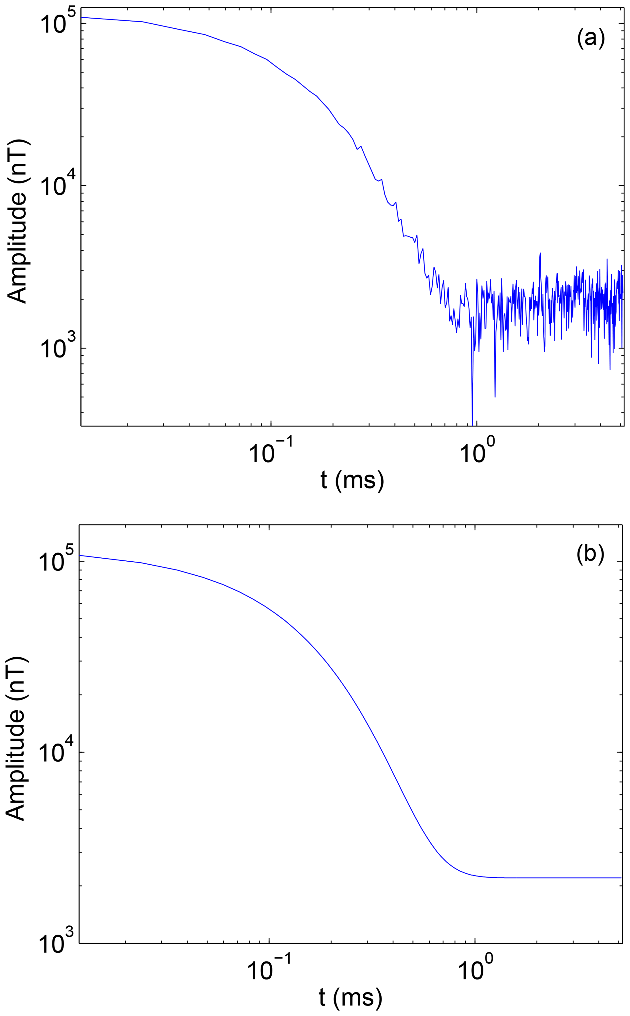
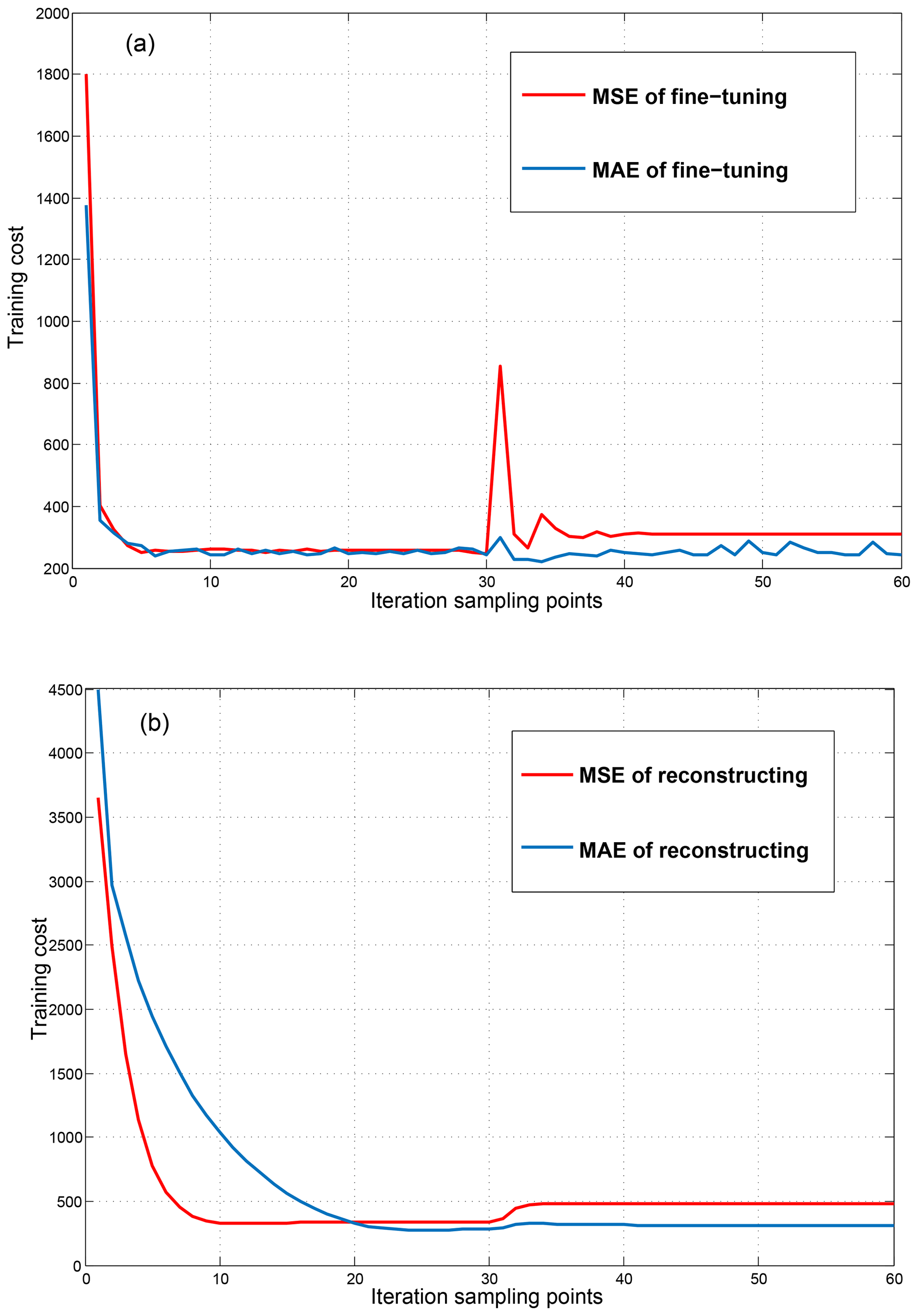
Figure 4 The training cost comparison of MAE and MSE (mean squared error): (a) is the training cost of fine-tuning, and (b) is the training cost of reconstructing.

Table 1 The training cost of the combination of learning rate and regularization rate. The value represents the MAE of the first 50 data points. Based on experience, about the first 50 data points have a better effect for extracting time-domain order waveforms. The best combination result of the learning rate and the regularization rate is the smallest value, which is shown in bold.

Therefore, based on the study of the distribution characteristics of the secondary field signal and autoencoder denoising method, we propose SFSDSA, which is a deep learning model of transient electromagnetic signal denoising.

1. SFSDSA will be stacked by multiple AEs to form a deep neural network of multilayer undercomplete encoding, and multiple AEs are used as a higher-order feature extraction part, which can utilize its deep structure to maximize the characteristics of the secondary field signal.

2. Based on the principle of DAEs, SFSDSA will set the secondary field measured data (received data) as the input data, and the geophysical inversion method is used to process the measured data of the secondary field to obtain the inversion signal as the clean signal data. SFSDSA maps the signal points of the noise interference to the high-probability points with a clean signal as reference according to the deep characteristics of the signal. Because maintaining the original data dimension is especially important for the undistorted processing and post-processing of the signal, it is necessary to set the original dimension after the last coding as the output layer dimension. Although the output method may produce the decoding loss, it can have high abstract retention of the secondary field signal characteristics and map the affected signal points to the high-probability position points.

3. The problem of too many nodes dying is a general disadvantage for rectified linear unit (RELU) activation function, and improved RELU activation functions like Leaky RELU all consistently outperform the RELU function in some tasks (Xu et al., 2015). Therefore, it is necessary to apply the improved RELU function to reduce the impact of the shortcomings of the RELU function. We choose the scaled exponential linear units (SELUs) that have the capability of overcoming vanishing and exploding gradient problems in a sense and preform the best in full connection networks (Klambauer et al., 2017). We chose the Adam algorithm, which has the advantages of calculating different adaptive learning rates for different parameters and requiring little memory (Kingma and Ba, 2014). The SFSDSA model will address the problem of overfitting due to increased depth and the problem of only learning an identity function, because the regularized loss is introduced.

3 Mathematical derivation of SFSDSA

Firstly, the secondary field data (actual detection signal) are treated as a noisy input. Since the secondary field data are mainly a time-amplitude value, we can sample the signal as a point-amplitude value, in the form of matrix A; the dimensions are 1×N:

$$\begin{array}{}\text{(1)}& A=\left[\begin{array}{ccccc}{a}_{\mathrm{11}}& a_{\mathrm{12}}& \mathrm{\cdots }& a_{\mathrm{1}n-\mathrm{1}}& a_{\mathrm{1}n}\end{array}\right].\end{array}$$

Secondly, the geophysical inversion method is used to obtain the theoretical signal, which can be used as a clean signal, and then the theoretical signal is sampled as a point-amplitude value, in the form of matrix $\stackrel{\mathrm{̃}}{A}$; the dimensions are 1×N:

$$\begin{array}{}\text{(2)}& \stackrel{\mathrm{̃}}{A}=\left[\begin{array}{ccccc}{\stackrel{\mathrm{̃}}{a}}_{\mathrm{11}}& {\stackrel{\mathrm{̃}}{a}}_{\mathrm{12}}& \mathrm{\cdots }& {\stackrel{\mathrm{̃}}{a}}_{\mathrm{1}n-\mathrm{1}}& {\stackrel{\mathrm{̃}}{a}}_{\mathrm{1}n}\end{array}\right].\end{array}$$

Thirdly, the SFSDSA training model can be built, and Adam, which is a stochastic gradient descent (SGD) method, is applied to prevent gradient disappearance; regularization loss is used to prevent overfitting; and the SELU activation function is utilized to prevent too many points of death.

$$\begin{array}{}\text{(3)}& g_{\mathit{\theta }}\left(a_{\mathrm{1}n}\right)=f_{\mathrm{SELU}}(W{a}_{ln}+b),\end{array}$$

$$\begin{array}{}\text{(4)}& g_{\mathit{\theta }}\left(a_{\mathrm{1}n}\right)=\mathit{\lambda }\left\{\begin{array}{lr}W{a}_{\mathrm{1}n}+b& a_{\mathrm{1}n}>\mathrm{0}\\ \mathit{\alpha }{e}^{W{a}_{\mathrm{1}n}+b}-\mathit{\alpha }& a_{\ln }<=\mathrm{0}\end{array},\right.\end{array}$$

where $\mathit{\theta }=(w,b)$, w denotes the $N\times N{}^{\prime }$ parameter matrix ($N{}^{\prime }<N$) and b denotes the offset of the N^′ dimensions. After the first compression coding layer, the signal is the extracted feature and is represented as the $\mathrm{1}\times N{}^{\prime }$ parameter matrix. In order to extract high-level features while removing as much noise as possible and other factors, we can compress again.

$$\begin{array}{}\text{(5)}& g_{\mathit{\theta }{}^{\prime }}\left(a{{}^{\prime }}_{\mathrm{1}N{}^{\prime }}\right)=\mathit{\lambda }\left\{\begin{array}{lr}W{}^{\prime }a{{}^{\prime }}_{\mathrm{1}N{}^{\prime }}+b{}^{\prime }& a{{}^{\prime }}_{\mathrm{1}N{}^{\prime }}>\mathrm{0}\\ \mathit{\alpha }{e}^{W{}^{\prime }a{{}^{\prime }}_{\mathrm{1}N{}^{\prime }}+b{}^{\prime }}-\mathit{\alpha }& a{{}^{\prime }}_{\mathrm{1}N{}^{\prime }}<=\mathrm{0}\end{array}\right.\end{array}$$

W denotes the $N{}^{\prime }\times N{}^{\prime \prime }$ parameter matrix ($N{}^{\prime \prime }<N{}^{\prime }$) and b denotes the offset of the N^′′ dimensions, and the features of the actual detection signal are extracted again after more feature extraction layers can be stacked. For the secondary field signal, it is necessary to maintain the same input and output dimensions to ensure that the signal is not distorted and later processed. When feature extraction reaches a certain extent, it is necessary to reconstruct back to input dimensions.

Reconstruction can be regarded as the process that the noisy signal points map back to the original dimensions after the features are highly extracted. At the same time, reconstruction is the process of signal characteristic amplification. Finally output matrix $\overline{A}$ with the same dimensions as the inputs can be retrieved:

$$\begin{array}{}\text{(6)}& \overline{A}=\left[\begin{array}{ccccc}{\overline{a}}_{\mathrm{11}}& {\overline{a}}_{\mathrm{12}}& \mathrm{\cdots }& {\overline{a}}_{\mathrm{1}n-\mathrm{1}}& {\overline{a}}_{\mathrm{1}n}\end{array}\right].\end{array}$$

The output $\overline{A}$ we obtained can be used to get the loss from the clean signal $\stackrel{\mathrm{̃}}{A}$ using the loss function. The general loss function has the squared loss, which is mostly used in the linear regression problem. However, the secondary field data are mostly nonlinear, and the absolute loss is used in this paper:

$$\begin{array}{}\text{(7)}& L(\overline{A},\stackrel{\mathrm{̃}}{A})=|\overline{A}-\stackrel{\mathrm{̃}}{A}|.\end{array}$$

In the meantime, regularization loss optimization is used in this paper in order to avoid the problem of overfitting, and then

$$\begin{array}{ll}{\displaystyle }\mathrm{loss}& {\displaystyle }={\mathit{\theta }}^{\ast },{{\mathit{\theta }}^{\prime }}^{\ast }={\arg }_{\mathit{\theta },\mathit{\theta }{}^{\prime }}min{\displaystyle \frac{\mathrm{1}}{n}}\sum _{i=\mathrm{1}}^{n}L(x^i,g_{\mathit{\theta }{}^{\prime }}(f_{\mathit{\theta }}\left(x^i\right)\left)\right)\\ \text{(8)}& {\displaystyle }& {\displaystyle }+\mathit{\lambda }R\left(w\right).\end{array}$$

After the loss is calculated, the Adam algorithm is used to reverse the optimization of parameters.

Figure 5 Training cost of each process.

Figure 6 Iteration sampling points.

Figure 7 SFSDSA hidden layer number and MAE values.

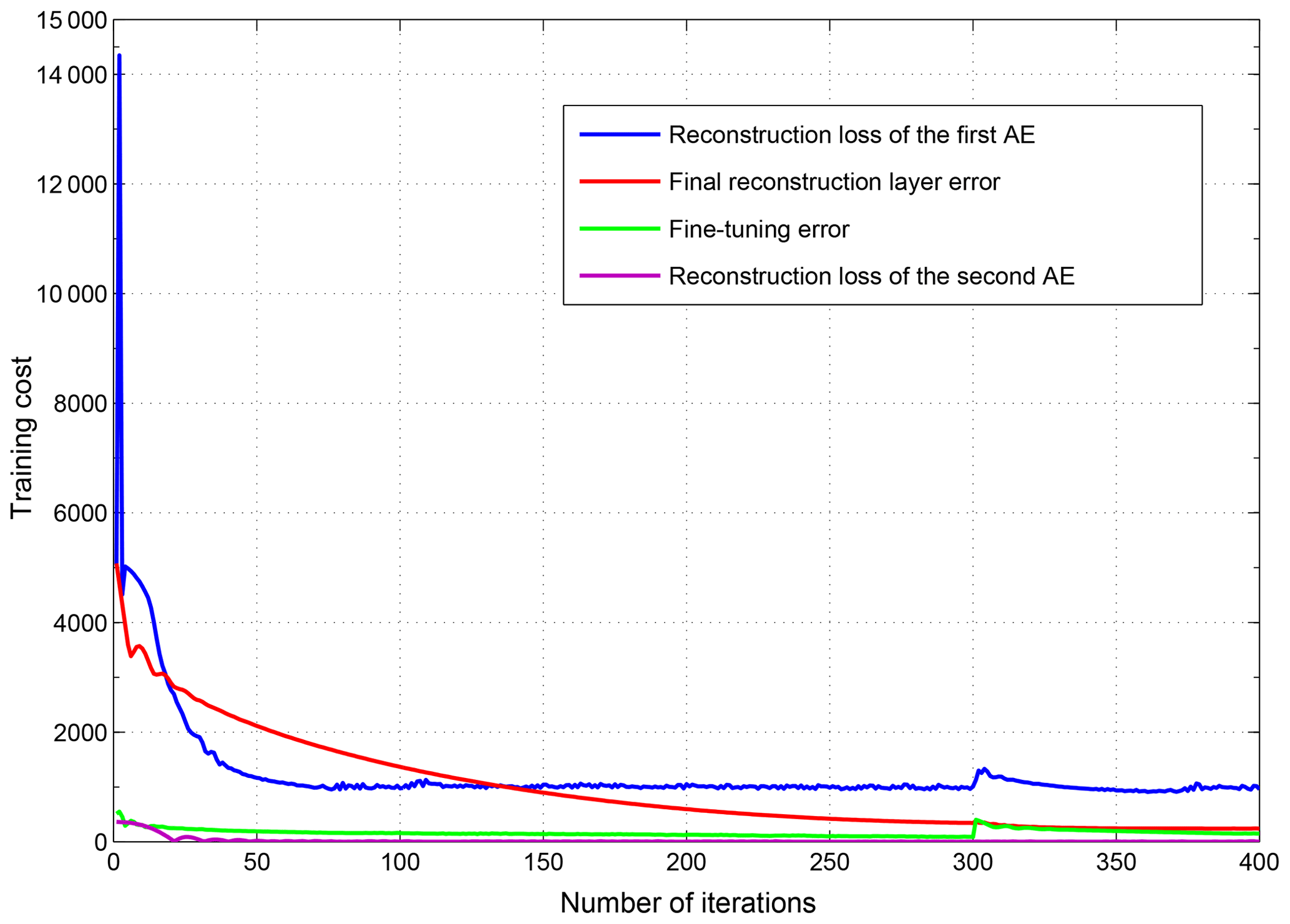
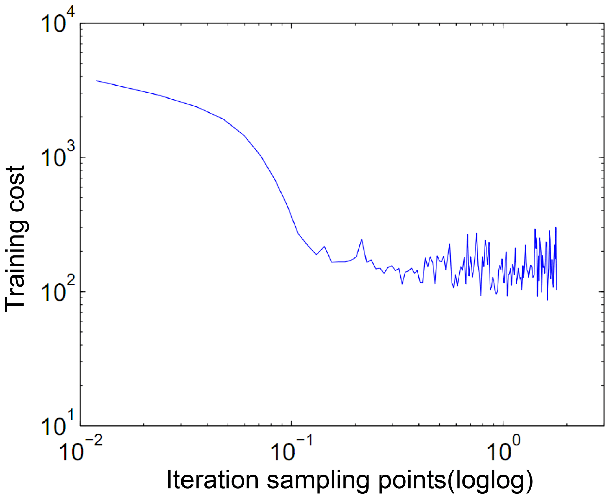
Figure 1 is the algorithm structure diagram of SFSDSA. With reference to the theory of DAEs, SFSDSA maps the signal points of the noise interference to the high-probability points with a clean signal as reference according to the deep characteristics of the signal, so as to realize the signal noise and reduce noise interference. This high-probability position is determined by the theoretical clean signal and the multilayer model of the feature extraction ability. The multilayer feature extraction preserves the deep feature of secondary field data, and the effect of noise is reduced.

For the noise suppression problem of the secondary field signal in the transient electromagnetic method, our goal is to extract the deep features of the secondary field signal and map the data points affected by noise to the estimated high-probability points according to their own signal features. We also found that the purpose of extracting the distribution characteristics of the secondary field signal data is similar to that of unsupervised learning.

Table 2 Comparison of MAE models.

4 Experiment and analysis

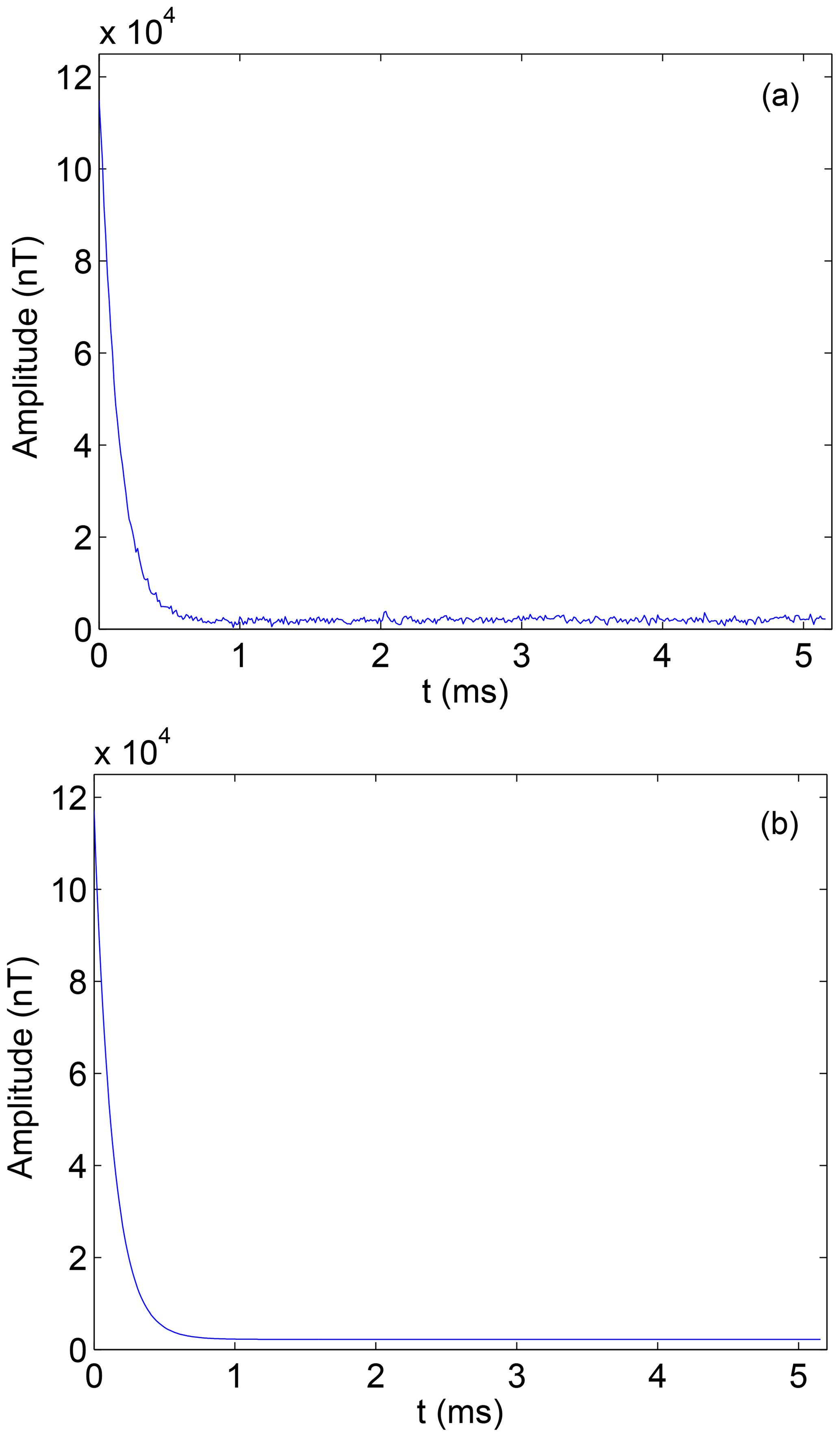
In this paper, the secondary field signal of a certain place is used as the experimental analysis signal. Usually, the secondary field signals can be obtained continuously on a period of time, so a large number of signals can be extracted conveniently as the training samples.The secondary field actual signals are extracted as 1×434 as input signals of noise pollution, as is shown in Fig. 2a. At the same time, based on the secondary field actual signals, the geophysical inversion method is used to obtain the theoretical detection signal as a clean signal uncontaminated by noise, as is shown in Fig. 2b. In order to be able to highlight the differences between the data, data are expressed in a double logarithmic form (loglog), as is shown in Fig. 3a and b.

The deep features of original data are extracted by feature extraction layers (compression coding layers). As the number of layers increases, SFSDSA can be a more complex abstract model with limited neural units (to get higher-order features for this small-scale input in this paper), and more feature extraction layers will inevitably lead to overfitting. Moreover, the reconstruction effect can be affected by the number of feature extraction layer nodes. If the SFSDSA model has too few nodes, the characteristics of the data can not be learned well. However, if the number of feature extraction layer nodes is too large, the designed lossy compression noise reduction can not be achieved well and the learning burden is increased.

Therefore, based on the aforementioned questions, we design the SFSDSA model (Fig. 1), and the number of nodes in the latter feature extraction layer is half the number of nodes in the previous feature extraction layer, until it is finally reconstructed back to the original dimension. The SFSDSA model is a layer-by-layer feature extraction, which can be regarded as the process of stacking AEs. Low dimensions are represented by the high-dimensional data features, which can learn the input features. At the same time, since the reconstruction loss is the loss of the output related to the clean signal, it can also be said that the input signal can be regarded as a clean signal based on the noise, the training measure of the DAE model increases the robustness of the model and reconstructs the lossy signal, and mapping the signal point to its high-probability location can be viewed as a noise reduction process.

Figure 8 Actual secondary field data after SFSDSA model noise reduction.

In the training experiment, we collected 2400 periods of transient electromagnetic method secondary field signals from the same collection location, and we selected 434 data points in each period. Meanwhile, 100 periods of signals are randomly acquired as a test and validation set for improving the robustness of the model. We use Google's deep learning framework – Tensorflow, which is used to build the SFSDSA model. The parameter settings for the model are as follows: batch size =8, epochs =2. We do a grid search and get the good parameter combination of learning rate and regularization rate as shown in Table 1 (learning rate =0.001 and regularization rate =0.15).

Figure 9 Specific points analysis.

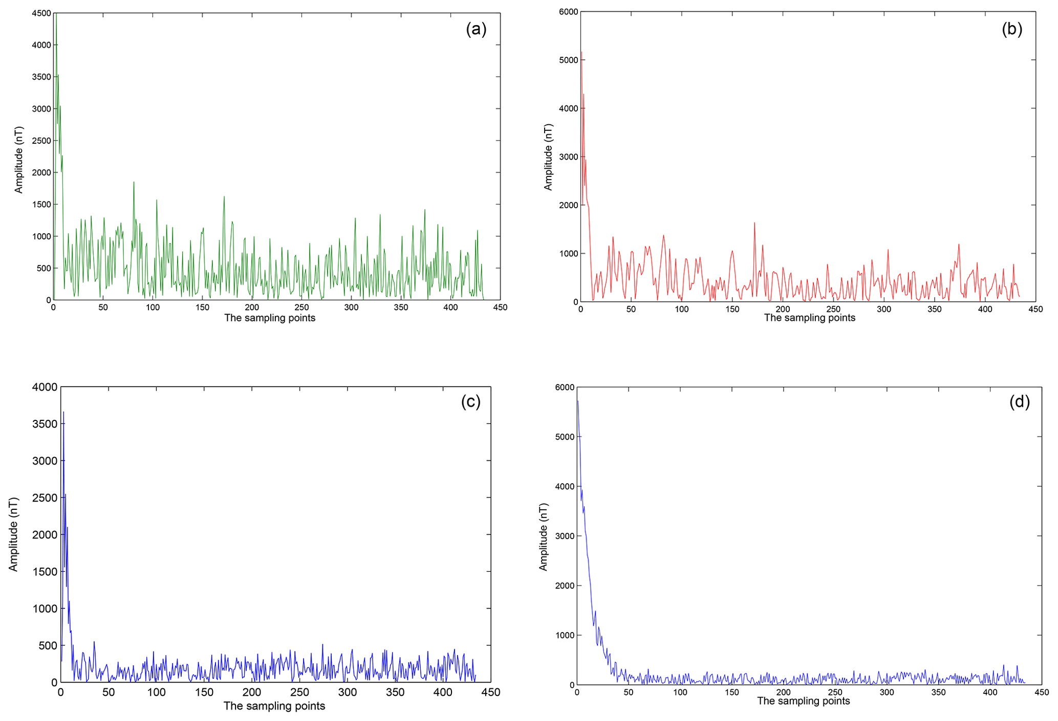
Figure 10 (a) Kalman filter. (b) Wavelet transform filter. (c) PCA filter. (d) SFSDSA denoising.

We analyzed and compared the selection of the two loss functions of mean absolute error (MAE) and mean squared error (MSE) in experiments as shown in Fig. 4. Meanwhile, according to the previous work and the SFS denoising task of the transient electromagnetic method, we think that MAE is a better choice. On the one hand, our task is to map the outliers affected by noise to the vicinity of the theoretical signal point; in other words, the model should ignore the outliers affected by noise to make it more consistent with the distribution of the overall signal. We know that MAE is quite resistant to outliers (Shukla, 2015). On the other hand, the squared error is going to be huge for outliers, which tries to adjust the model according to these outliers at the expense of other good points (Shukla, 2015). For signals that are subject to noise interference in the secondary field of the transient electromagnetic method, we do not want to overfit outliers that are disturbed by noise, but we want to treat them as data with noise interference. The evaluation index is the mean absolute error of output reconstruction data and clean input data. The smaller the MAE, the closer the output reconstruction data are to the theoretical data. The model also performs better in noise reduction.

$$\begin{array}{}\text{(9)}& \mathrm{MAE}(x,y)={\displaystyle \frac{\mathrm{1}}{m}}\sum _{i=\mathrm{1}}^m\left|h\right(x{)}^{\left(i\right)}-y^{\left(i\right)}|,\end{array}$$

where x denotes the noise interference data, m denotes the number of sampling points, h denotes the model and y denotes theoretical data.

Figure 11 The geographic distribution of the collection points (first to seventh).

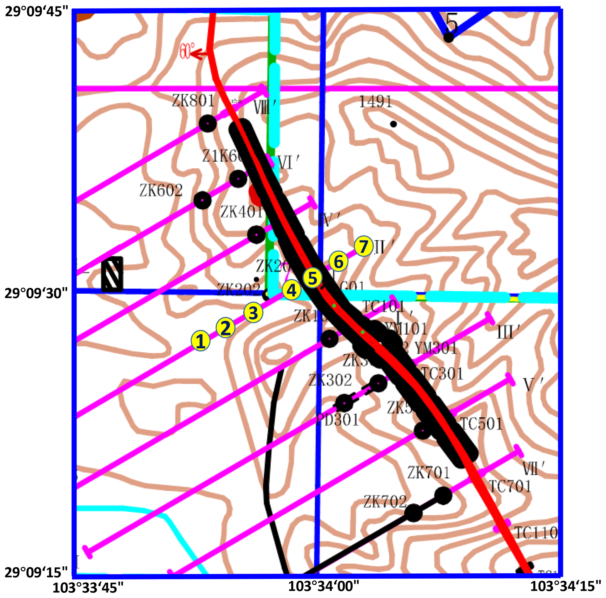
Figure 12 (a) The original 30th to 50th points from seven actual detecting locations. (b) The denoising 30th to 50th points from seven actual detecting locations.

In the previous experiments, we set hyper-parameters (batch size =8, learning rate =0.1, regularization rate =0, epochs =20) based on experience, but we initially take the measure of a small number of epochs (epochs =2) according to the experiment. We added the experiment as shown in Fig. 5 to support our standpoint. The model oscillates quickly and converges. Training with fewer epochs can avoid useless training and overfitting, maintaining the distribution characteristics of the signal itself. As shown in Fig. 6, the reconstruction error oscillates and converges as the training progresses. This phenomenon is similar to the tail of the actual signal. We try to stop training when the convergence occurs; the idea similar to early stopping makes the model more robust (Caruana et al., 2000).

By analyzing Fig. 7, the relationship between MAE and the number of hidden layers, we found that the result of stacking two AEs has a good effect. We guess that the size of the AE hidden layer is too small after multiple stacking (for instance, the fourth AE only has 27 nodes because the size of the latter AE is half that of the previous AE in order to extract the better feature), and the representation of signal characteristics is not complete, resulting in large reconstruction costs. If we want to get a better result, more iterations may be used but this tends to cause overfitting. Meanwhile, we found that the reconstruction loss of the second AE is already very small (shown in Fig. 5). So it is not necessary to stack more AEs.

The training time will be less when the small-scale deep learning model is applied. By analyzing Fig. 2a, we found that, because the amplitude of the tail of the actual signal is small and the influence of the noise is significant, the tail of the signal oscillates violently. Meanwhile, after the feature extraction and noise reduction to a certain extent, the noise interference can not be completely removed, the reconstruction can not completely present the clean signal and it is only possible to map the signal points as high-probability points to reduce reconstruction loss.

4.1 Training results

After several experiments, the MAE of actual signals fell from 534.5 to about 215. Compared with the secondary field actual signals and signals denoised by the SFSDSA model, the noise reduction effect of SFSDSA is obvious in Fig. 8.

The 35th to 55th points are selected for specific analysis in Fig. 7. Through noise reduction in the training SFSDSA model, the singular points (large amplitude deviation from theoretical signal) affected by the noise are mapped to the high-probability positions (e.g., point no. 38 and point no. 51). This process is the process of damage reconstruction that the DAE model has verified. At the same time, our stacked AE model also keeps extracting the features, and the singular points are restored to the corresponding points according to the characteristics of the data. The whole process realizes the noise reduction of the secondary field actual signal based on the secondary field theoretical signal, and the model maps the singular points to locations where there is a high probability of occurrence, which is also similar to the most estimative method based on observations and model predictions by Kalman filtering.

5 Comparison with traditional noise reduction methods

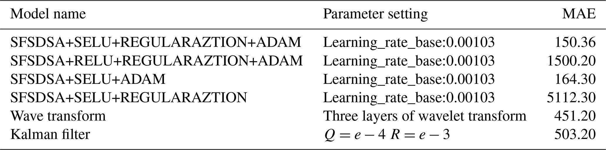
We also conducted wavelet transform, PCA and Kalman filter method experiments, in which the number of layers of the wavelet transform is three, called DWT() and construction function IDWT() in Matlab. By using the PCA method, we perform the experiment to verify the effect of noise reduction. But the process of programming is more complicated when using mathematical derivation, so we use the scikit-learn library to realize noise reduction. Kalman filtering is implemented in Python, where the system noise Q is set to 1e−4 and the measurement noise R is set to 1e−3. Figure 10 shows the absolute error distribution for that method. We can find from the figure model of noise reduction based on the SFSDSA model of secondary field data that the SFSDSA model is better than Kalman filter, wavelet transform and PCA methods. At the same time, as the Kalman filter is a linear filter, its noise reduction effect is very poor in this paper. Moreover, the underlying structure is not easy to modify, resulting in the scikit-learn library being unable to adjust parameters adaptively based on signal characteristics. After the filtering test, and then the MAE corresponding to the calculation of the theoretical data, it can be seen that the effect of PCA filtering is lower than that of SFSDSA.

At the same time, we compared the optimization results of various models using the traditional method with those of the SFSDSA model, as shown in Table 2.

Figure 11 is the diagram of the mine where the exploration experiment was conducted. The thick red curve is the actual mine vein curve. A data collection survey line, which is the southwest–northeast pink curve shown in the figure, is designed with seven points marked as number 1 to 7 along it, and the distance between each point is 50 m.

In the data analysis, we analyzed the first 50 points in the second field, which were collected in the actual mine. The early signal of the secondary field is stronger than the later one, and it is not easily disturbed by the noises. So in Fig. 12 we take out the later 21 points in each collection point, which are used for further analysis. Figure 12a shows extracted time-domain order waveforms formed by the actual data acquired at the seven collection points at the same time. Figure 12b shows extracted time-domain order waveforms formed by the data denoised by the SFSDSA model. By comparing the two images in Fig. 12, it can be clearly seen that the curves in Fig. 12a have obvious intersections, and the intersections in Fig. 12b are almost invisible. In the transient electromagnetic method, the intersected curve can not indicate the deeper underground geological information. It can be explained that the curve after the denoising model can reflect the deep geological information.

6 Conclusions

Based on the transient electromagnetic method, the deep-seated information is reflected in the late stage of the second field signal when deep-level surveys are conducted, but the late-stage signals are very weak and easily contaminated by noise. Therefore, we use the measured data for modeling to obtain the theoretical model, which will perform noise reduction based on the geological features represented by the previous training data set. Meanwhile, it is necessary to analyze the known geological features carefully and apply the model according to the actual geological conditions before using our method. And this method has a good generalization for different collection points of the same geological feature area. By introducing the deep learning algorithm integrated with the characteristics of the secondary field data, SFSDSA can map the contaminated signal to a high-probability position. By comparing several filtering algorithms by using same sample data, the SFSDSA method has better performance and the denoising signal is conducive to further improving the effective detection depth.