the Creative Commons Attribution 4.0 License.
the Creative Commons Attribution 4.0 License.
 | 29 Mar 2018
Utsu aftershock productivity law explained from geometric operations on the permanent static stress field of mainshocks
The aftershock productivity law is an exponential function of the form K∝exp(αM), with K being the number of aftershocks triggered by a given mainshock of magnitude M and α≈ln (10) being the productivity parameter. This law remains empirical in nature although it has also been retrieved in static stress simulations. Here, we parameterize this law using the solid seismicity postulate (SSP), the basis of a geometrical theory of seismicity where seismicity patterns are described by mathematical expressions obtained from geometric operations on a permanent static stress field. We first test the SSP that relates seismicity density to a static stress step function. We show that it yields a power exponent q = 1.96 ± 0.01 for the power-law spatial linear density distribution of aftershocks, once uniform noise is added to the static stress field, in agreement with observations. We then recover the exponential function of the productivity law with a break in scaling obtained between small and large M, with α=1.5ln (10) and ln (10), respectively, in agreement with results from previous static stress simulations. Possible biases of aftershock selection, proven to exist in epidemic-type aftershock sequence (ETAS) simulations, may explain the lack of break in scaling observed in seismicity catalogues. The existence of the theoretical kink, however, remains to be proven. Finally, we describe how to estimate the solid seismicity parameters (activation density δ+, aftershock solid envelope r∗ and background stress amplitude range Δo∗) for large M values.
- Article
(4947 KB) - Full-text XML
- BibTeX
- EndNote


Aftershocks, one of the most studied patterns observed in seismicity, are characterized by three empirical laws, which are functions of time, such as the modified Omori law (e.g., Utsu et al., 1995), space (e.g., Richards-Dinger et al., 2010; Moradpour et al., 2014) and mainshock magnitude (Utsu, 1970a, b; Ogata, 1988). The present study focuses on the latter relationship, i.e., the Utsu aftershock productivity law, which describes the total number of aftershocks K produced by a mainshock of magnitude M as
with m0 the minimum magnitude cutoff (Utsu, 1970b; Ogata, 1988). This relationship was originally proposed by Utsu (1970a, b) by combining two other empirical laws, the Gutenberg–Richter relationship (Gutenberg and Richter, 1944) and Båth's law (Båth, 1965), respectively:
with N the average number of events above magnitude m, A a seismic activity constant, β the magnitude size ratio (or in base-10 logarithmic scale) and ΔmB the magnitude difference between the mainshock and its largest aftershock, such that
with and α≡β. Equation (3) was only implicit in Utsu (1970a) and not exploited in Utsu (1970b), where K0 was fitted independently of the value taken by Båth's parameter ΔmB. The α value was in turn decoupled from the β value in later studies (e.g., Seif et al., 2017 and references therein).
Although it seems obvious that Eq. (1) can be explained geometrically if the volume of the aftershock zone is correlated to the mainshock surface area S with
(Kanamori and Anderson, 1975; Yamanaka and Shimazaki, 1990; Helmstetter, 2003), there is so far no analytical, physical expression of Eq. (1) available. Although Hainzl et al. (2010) retrieved the exponential behavior in numerical simulations where aftershocks were produced by the permanent static stress field of mainshocks of different magnitudes, it remains unclear how K0 and α relate to the underlying physical parameters.
The aim of the present article is to describe the Utsu aftershock productivity equation (Eq. 1) in terms of a geometrical theory of seismicity coined “solid seismicity”, where the Eq. (4) scaling is parameterized using the solid seismicity postulate (SSP). The SSP has already been shown to effectively explain other empirical laws of both natural and induced seismicity from simple geometric operations on a permanent static stress field (Mignan, 2012, 2016a). The theory is applied here for the first time to describe aftershocks.
2.1 Demonstration of the productivity law by geometric operations
“Solid seismicity”, a geometrical theory of seismicity, is based on the
following postulate (Mignan et al., 2007; Mignan, 2008, 2012,
2016a).
Solid seismicity postulate: Seismicity can be strictly categorized into three regimes of constant spatiotemporal densities δ – background δ0, quiescence δ− and activation δ+ (with ) – occurring respective to the static stress step function:
with σ the static stress (stress unit), Δo∗ the background stress amplitude range (stress unit), a stress threshold value separating two seismicity regimes, and δ
the spatial density of events (number of events per unit of volume) per seismicity regime.
We mean by “strictly categorized” that any seismicity population is either part of the background, quiescence or activation regime (or class), with no other regime or class possible (i.e., a sort of hard labeling). Based on this postulate, Mignan (2012) demonstrated the power-law behavior of precursory seismicity in agreement with the observed time-to-failure equation (Varnes, 1989), while Mignan (2016a) demonstrated both the observed parabolic spatiotemporal front and the linear relationship with injection flow rate of induced seismicity (Shapiro and Dinske, 2009). It remains unclear whether the SSP has a physical origin or not. If not, it would still represent a reasonable approximation of the linear relationship between event production and static stress field in a simple clock-change model (Hainzl et al., 2010; Fig. 1a). For the testing of the SSP on the observed spatial distribution of aftershocks, see Sect. 2.2. The power of Eq. (5) is that it allows seismicity patterns to be defined in terms of “solids” described by the spatial envelope , where r is the distance from the static stress source (e.g., mainshock rupture) and r∗ is the distance r at which there is a change of regime (quiescence–background at or background–activation at . The spatiotemporal rate of seismicity is then a mathematical expression defined by the density of events δ times the volume characterized by r∗ (see previous demonstrations in Mignan et al., 2007 and Mignan, 2011, 2012, 2016a where simple algebraic expressions were obtained).
In the case of aftershocks, we define the static stress field of the mainshock by
with Δσ0 < 0 the mainshock stress drop, c the crack radius and r the distance from the crack. Equation (6) is a simplified representation of stress change from slip on a planar surface in a homogeneous elastic medium. It takes into account both the square root singularity at crack tip and the 1∕r3 falloff at higher distances (Dieterich, 1994; Fig. 1b). It should be noted that this radial static stress field does not represent the geometric complexity of Coulomb stress fields (Fig. 2a). However, we are here only interested in the general behavior of aftershocks with Eq. (6) retaining the first-order characteristics of this field (i.e., on-fault seismicity; Fig. 2b), which corresponds to the case where the mainshock relieves most of the regional stresses and aftershocks occur on optimally oriented faults. It is also in agreement with observations, most aftershocks being located on and around the mainshock fault traces in southern California (Fig. 2c; see Sect. 3). The occasional cases where aftershocks occur off-fault (e.g., Ross et al., 2017) can be explained by the mainshock not relieving all of the regional stress (King et al., 1994; Fig. 2d).
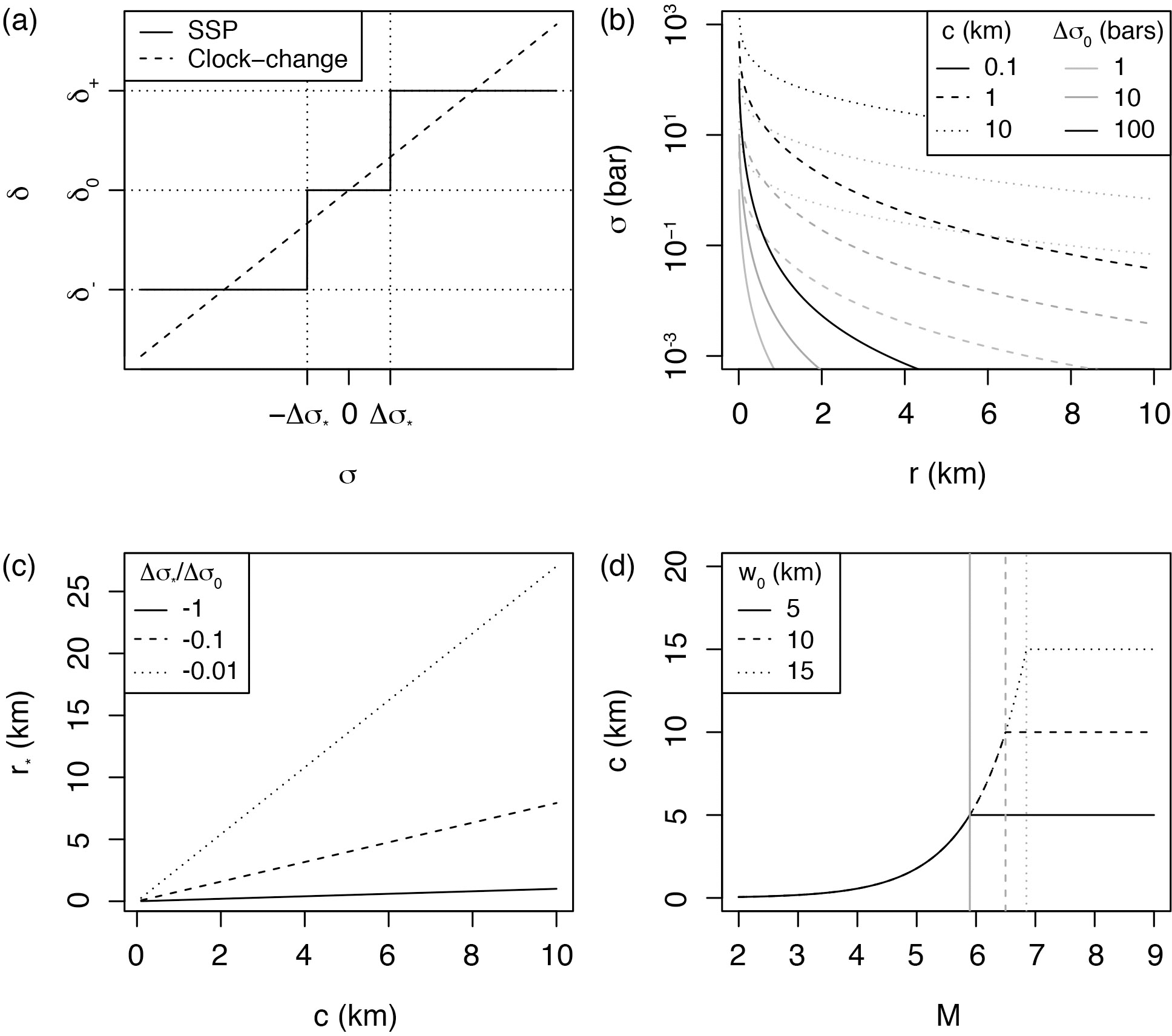
Figure 1Definition of the aftershock solid envelope in a permanent static stress field: (a) event density stress step-function δ(σ) (Eq. 5) of the solid seismicity postulate (SSP) in comparison to the linear clock-change model; (b) static stress σ versus distance r for different effective crack radii c and rupture stress drops Δσ0 (Eq. 6); (c) linear relationship between effective crack radius c and aftershock solid envelope radius r∗ for different ratios (Eq. 7); (d) relationship between mainshock magnitude M and effective crack radius c for different seismogenic widths w0 (Eq. 8).
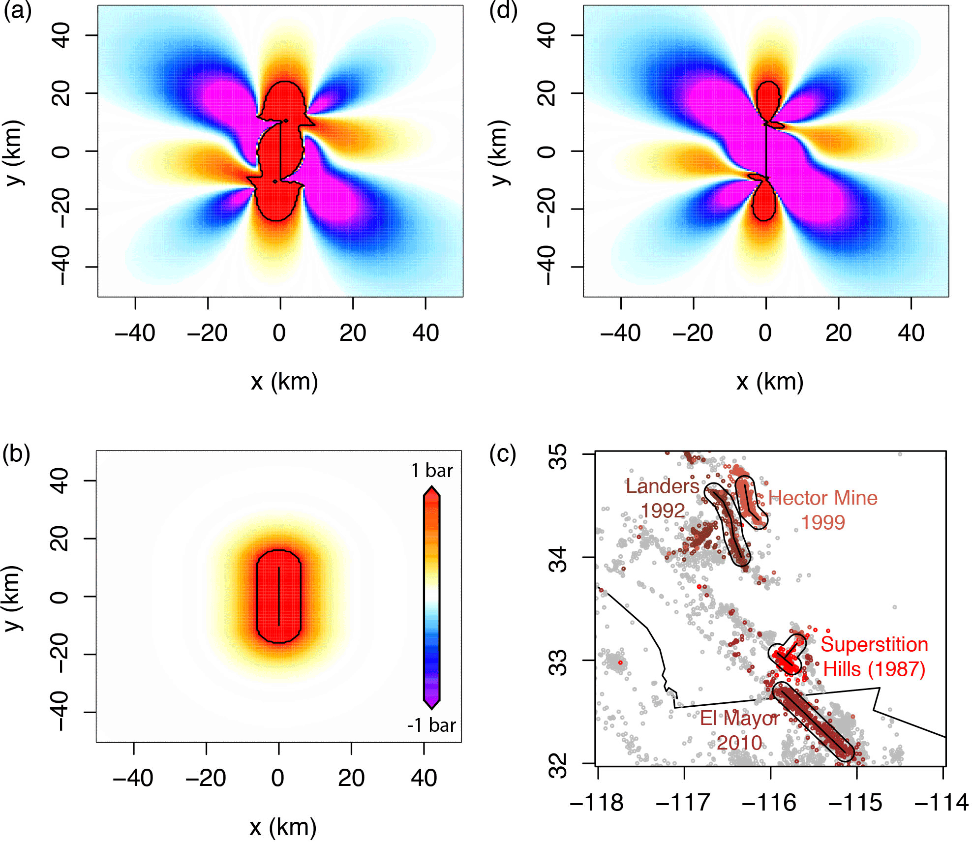
Figure 2Possible static stress fields and inferred aftershock spatial distribution: (a) right-lateral Coulomb stress field for optimally oriented faults, where the mainshock relieves all of the regional stresses σr=10 bar, with bar ( bar the shear modulus, s=0.6 m the slip, L=20 km the fault length and w=10 km the fault width); (b) radial static stress field computed from Eq. (6) with bar and for consistency with panel (a); (c) aftershock distribution of the largest strike-slip events in the southern California relocated catalog, identified here as all events occurring within 1 day of the mainshock (see data Sect. 3.1); (d) right-lateral Coulomb stress field for optimally oriented faults, where the mainshock relieves only a fraction of the regional stresses σr=100 bar with bar (same rupture as in panel a) – the black contour represents 1 bar in panels (a), (b) and (d) and a 10 km distance from rupture in panel (c). Coulomb stress fields of panels (a) and (d) were computed using the Coulomb 3 software (Lin and Stein, 2004; Toda et al., 2005).
For , Eq. (6) yields the aftershock solid envelope of the following form:
function of the crack radius c and of the ratio between background stress amplitude range Δo∗ and stress drop Δσ0 (Fig. 1c). With Δσ0 independent of earthquake size (Kanamori and Anderson, 1975; Abercrombie and Leary, 1993) and Δo∗ assumed constant, r∗ is directly proportional to c with proportionality constant, or stress factor, F (Eq. 7). Geometrical constraints due to the seismogenic layer width w0 then yield
with S the rupture surface area defined by Eq. (4) and c becoming an effective crack radius (Kanamori and Anderson, 1975; Fig. 1d). Note that the factor of 2 (i.e., using w0 instead of w0∕2) comes from the free surface effect (e.g., Kanamori and Anderson, 1975; Shaw and Scholz, 2001).
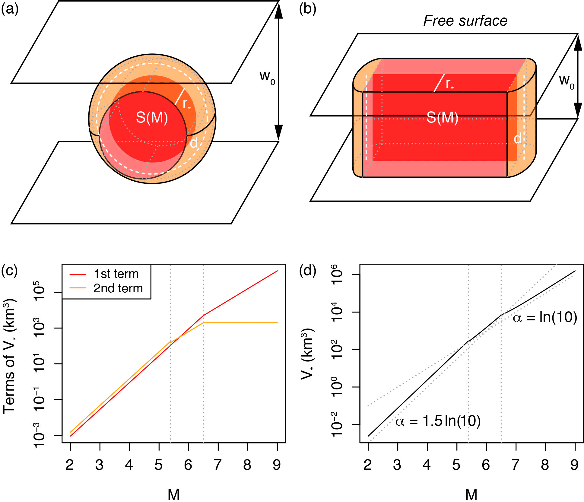
Figure 3Geometric origin of the aftershock productivity law: (a) sketch of the aftershock solid for a small mainshock rupture represented by a disk; (b) sketch of the aftershock solid for a large mainshock rupture represented by a rectangle; (c) relative role of the two terms of Eq. (9), here with w0=10 km and (to first estimate c and r∗ from Eqs. 8 and 7, respectively); (d) aftershock productivity law (normalized by δ+) predicted by solid seismicity (Eq. 11). This relationship is of the same form as the Utsu productivity law (Eq. 1) for large M (see text for an explanation of the lack of break in scaling in Eq. 1 for small M). Dotted vertical lines represent M for and , respectively.
The aftershock productivity K(M) is then the activation density δ+ times the volume V∗(M) of the aftershock solid. For the case in which the mainshock relieves most of the regional stress, stresses are increased all around the rupture (King et al., 1994), which is topologically identical to stresses increasing radially from the rupture plane (Fig. 2a–b). It follows that the aftershock solid can be represented by a volume of contour r∗(M) from the rupture plane geometric primitive, i.e., a disk or a rectangle for small and large mainshocks, respectively. This is illustrated in Fig. 3a–b and can be generalized by
where d is the distance traveled around the geometric primitive by the geometric centroid of the semicircle of radius r∗(M) (i.e., Pappus's Centroid Theorem), or
For the disk, the volume (Eq. 9) corresponds to the sum of a cylinder of radius c(M) and height 2r∗(M) (first term) and of half a torus of major radius c(M) and minus radius r∗(M) (second term). For the rectangle, the volume is the sum of a cuboid of length l(M) (i.e., rupture length), width w0 and height 2r∗(M) (first term) and of a cylinder of radius r∗(M) and height w0 (second term; see red and orange volumes, respectively, in Fig. 3a–c). Finally inserting Eqs. (7), (8) and (10) into Eq. (9), we obtain
which is represented in Fig. 3d. Considering the two main regimes only (small versus large mainshocks) and inserting Eq. (4) into (11), we get
which is a closed-form expression of the same form as the original Utsu productivity law (Eq. 1). Note that K and δ+ are both, implicitly, functions of the selected minimum aftershock magnitude threshold m0.
Here, we predict that the α value decreases from to ln (10)≈2.30 when switching regime from small to large mainshocks (or from 1.5 to 1 in a base-10 logarithmic scale). It should be noted that Hainzl et al. (2010) observed the same break in scaling in static stress transfer simulations, which corroborates our analytical findings. Hainzl et al. (2010) simulated aftershocks using the clock-change model where events were advanced in time by the static stress change produced by a mainshock in a 3-D medium. They explained the scaling break observed in simulation as a transition from 3-D to 2-D scaling regime when the mainshock rupture dimension approached w0, which is compatible with the present demonstration. For large M, the scaling is fundamentally the same as in Eq. (4). Since that relation also explains the slope of the Gutenberg–Richter law (see physical explanation given by Kanamori and Anderson, 1975), it follows that α≡β, which is also in agreement with the original formulation of Utsu (1970a, b; Eq. 3).
2.2 Testing of the SSP on the aftershock spatial distribution
The SSP predicts a step-like behavior of the aftershock spatial density for an idealized smooth static stress field (Fig. 4a–b), which is in disagreement with real aftershock observations. A number of studies have shown that the spatial linear density distribution of aftershocks ρ is well represented by a power law, expressed as
with r the distance from the mainshock and q the power-law exponent. This parameter ranges over (Felzer and Brodsky, 2006; Lipiello et al., 2009; Marsan and Lengliné, 2010; Richards-Dinger et al., 2010; Shearer, 2012; Gu et al., 2013; Moradpour et al., 2014; van der Elst and Shaw, 2015). Although Felzer and Brodsky (2006) suggested a dynamic stress origin for aftershocks, their results were later questioned by Richards-Dinger et al. (2010). Most of the studies cited above suggest that the q value is explained from a static stress process. As for the examples of aftershocks shown to be dynamically triggered (e.g., Fan and Shearer, 2016), they are too few to alter the aftershock productivity law and too remote to be consistently defined as aftershocks in cluster methods.
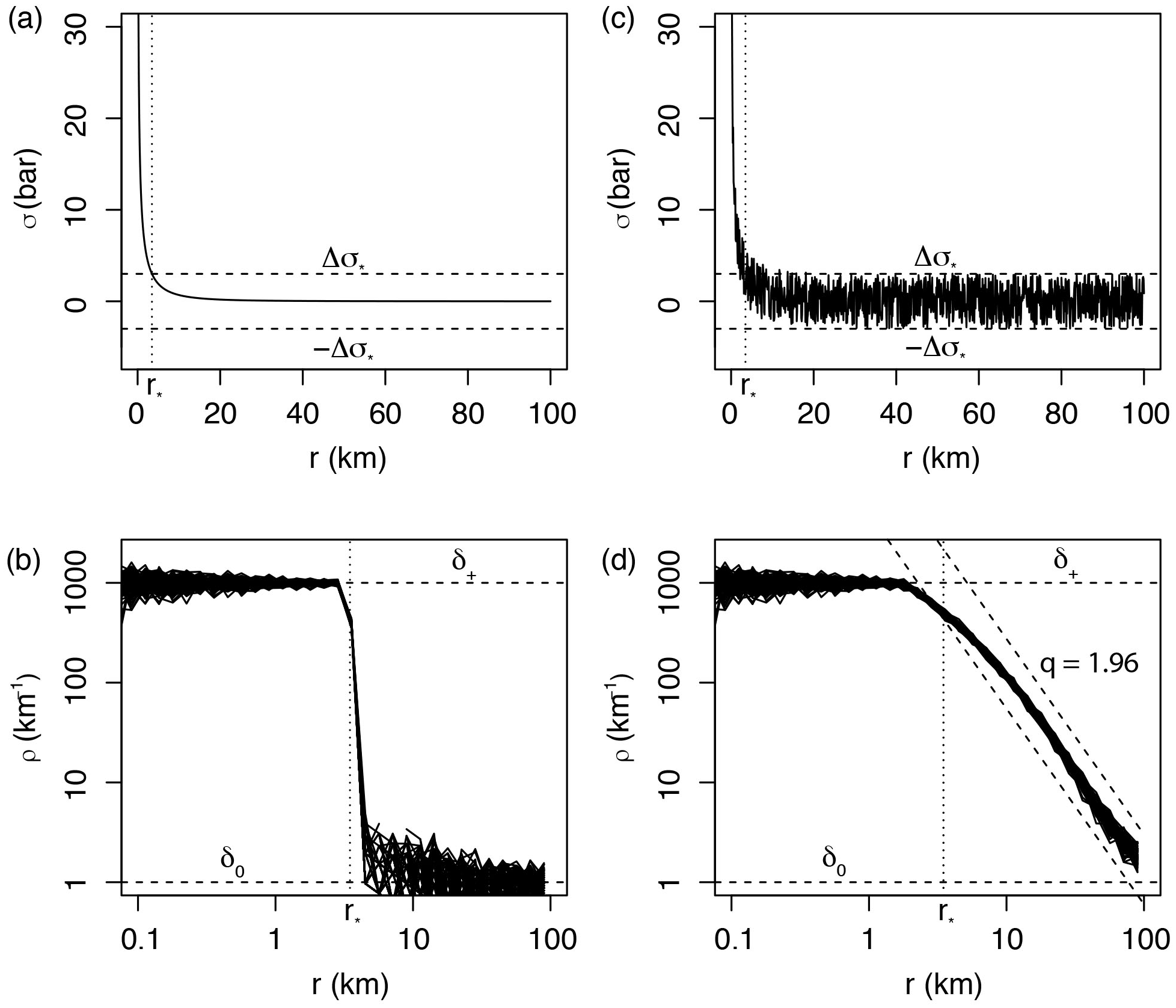
Figure 4Spatial distribution of aftershocks following the SSP: (a) Smooth static stress field as a function of distance r from the mainshock, with bar and c=10 km (Eq. 6); (b) step-like aftershock spatial linear density ρ(r) with event km−1, δ0=1 event km−1 and (ad hoc ratio yielding km; Eq. (7) – event distances sampled from the δ(r) distribution, repeated 100 times). Such distribution is not observed in nature; (c) same as panel (a) but with random uniform noise representative of spatial heterogeneities added to the regional stress field; (d) power-law-like aftershock spatial linear density ρ(r) with power exponent MLE estimate q=1.96, representative of real aftershock observations (see Fig. 5a), due to the addition of uniform noise to the static stress field.
In a more realistic setting, the static stress field must be heterogeneous (due to the occurrence of previous events and other potential stress perturbations). We therefore simulate the static stress field by adding a uniform random component bounded over following Mignan (2011) (see also King and Bowman, 2003). Note that any deviation above Δo∗ would be flattened to Δo∗ over time by temporal diffusion (the so-called “historical ghost static stress field” in Mignan, 2016a). Figure 4c shows the resulting stress field and Fig. 4d the predicted aftershock spatial density. Adding uniform noise blurs the contour of the aftershock solid, switching the aftershock spatial density from a step function (Fig. 4b) to a power law (Fig. 4d). We fit Eq. (13) to the simulated data using the maximum likelihood estimation (MLE) method with (Clauset et al., 2009) and find , in agreement with the aftershock literature. This result alone is, however, insufficient to prove the validity of the SSP.
3.1 Data
We consider the case of southern California and extract aftershock sequences from the relocated earthquake catalog of Hauksson et al. (2012) defined over the period 1981–2011, using the nearest-neighbor method (Zaliapin et al., 2008; used with its standard parameters originally calibrated for southern California, considering only the first aftershock generation). Only events with magnitudes greater than m0=2.0 are considered (a conservative estimate following results of Tormann et al., 2014; saturation effects immediately after the mainshock are negligible when considering entire aftershock sequences; Helmstetter et al., 2005).
3.2 Aftershock spatial density distribution
Figure 5a represents the spatial linear density distribution of aftershocks ρ(r) for the four largest strike-slip mainshocks in southern California: 1987 M=6.6 Superstition Hills, 1992 M=7.3 Landers, 1999 M=7.1 Hector Mine and 2010 M=7.2 El Mayor. The distance between mainshock and aftershocks is calculated as , with (x, y) the aftershock coordinates and (x0, y0) the coordinates of the nearest point to the mainshock fault rupture (as depicted in Fig. 2c). The dashed black lines shown in Fig. 5a are visual guides to q=1.96, showing that the SSP is compatible with real aftershock observations.
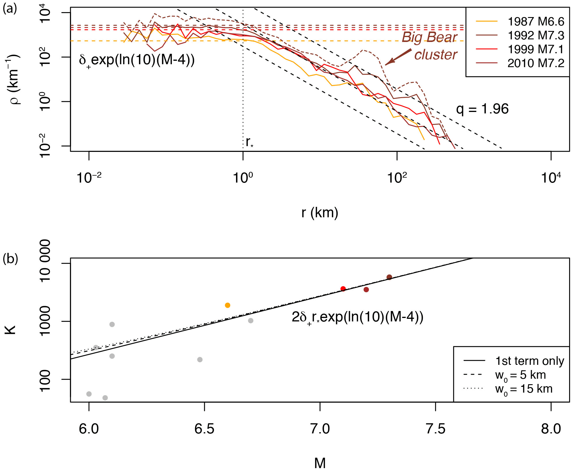
Figure 5Estimating the solid seismicity parameters from the spatial distribution of aftershocks: (a) spatial linear density distribution ρ(r) of aftershocks for the four largest strike-slip mainshocks in southern California (with first-generation aftershocks only; the density distribution comprising all aftershocks generated by the Landers mainshock is represented by the dotted curve to illustrate the type of spatial heterogeneity, such as the Big Bear cluster, not considered in the present study – see also Fig. 2c). The solid seismicity parameters km and event km−3 can be retrieved from the observed plateau ρ (r < r∗), in agreement with the SSP (see Fig. 4d). Note that the spatial power-law decay at high r is similar to the one expected by the SSP in the case of a static stress field with additive uniform noise (expected q=1.96 represented by the dashed black lines); (b) aftershock productivity K for M > 6. The curves represent the productivity law as defined by solid seismicity (Eq. 17) for different w0 values (first term only corresponds to w0=0; Eq. 18).
Comparing Fig. 5a to Fig. 4d suggests that r∗ can be roughly estimated from the spatial linear density plot, being the maximum distance r at which the plateau ends, here leading to 1 km. This parameter is constant for different large M values since both w0 and Δσ0 are constant while Δσ∗ is also a priori a constant. We can then estimate the ratio from Eq. (7). However, the result is ambiguous due to uncertainties in the width w0. For km, we get .
As for the plateau value ρ (r < r∗), it provides an estimate of the aftershock activation density δ+, with
a volumetric density, i.e., the linear density ρ normalized by the mainshock rupture area (Eq. 4). Due to the fluctuations in ρ (r < r∗), δ+ will be estimated from the productivity law instead (see Sect. 3.3), and ρ (r < r∗) will then be estimated from Eq. (14) (horizontal dashed colored lines), as detailed below.
It should be noted that we consider only the first-generation aftershocks to avoid ρ heterogeneities from secondary aftershock clusters occurring off-fault. An example of such heterogeneity and anisotropy is illustrated by the Landers–Big Bear case (Fig. 2c; dotted colored curve in Fig. 5a). Those cases are not systematic and therefore not considered in the aftershock productivity law. However, they are also due to static stress changes (e.g., King et al., 1994) with the anisotropic effects explainable by solid seismicity through the concept of historical ghost static stress field (Mignan, 2016a).
3.3 Aftershock productivity law
The observed number n of aftershocks of magnitude m≥m0 produced by a mainshock of magnitude M (for a total of N mainshocks) in southern California is shown in Figs. 5b (for large M≥6) and 6a (for the full range M≥m0). We fit Eq. (1) to the data using the MLE method with the log-likelihood function
for a Poisson process, representing the stochasticity of the count K of aftershocks produced by a mainshock at any given time. Inserting Eq. (1) in Eq. (15) yields
(note that the last term can be set to 0 during LL maximization). For southern California, we obtain αMLE=2.32 (1.01 in log10 scale) and K0=0.025 when considering large (M≥6) mainshocks only to avoid the issues of scaling break and data dispersion at lower magnitudes. This result, represented by the black solid line in Fig. 5b, is in agreement with previous studies in the same region (e.g., Helmstetter, 2003; Helmstetter et al., 2005; Zaliapin and Ben-Zion, 2013; Seif et al., 2017) and with predicted for large mainshocks in solid seismicity (Eq. 12). Moreover we find a bulk βMLE=2.34 (1.02 in log10 scale) (Aki, 1965), in agreement with α≡β.
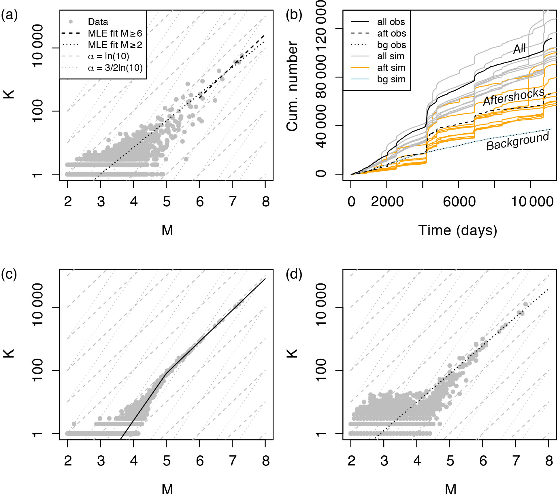
Figure 6Aftershock productivity defined as the number of aftershocks K(m0=2) per mainshock of magnitude M: (a) observed aftershock productivity in southern California with aftershocks selected using the nearest-neighbor method; (b) seismicity time series with distinction made between background events and aftershocks, observed (“obs”, in black) and ETAS-simulated (“sim”, colored); (c) true simulated aftershock productivity with kink, defined from Eq. (20); (d) retrieved simulated aftershock productivity with aftershocks selected using the nearest-neighbor method – data points in panels (a), (c) and (d) are represented by grey dots; the model MLE fits are represented by the dashed and dotted black lines for M ≥ 6 and M≥m0, respectively; dashed and dotted grey lines are visual guides to and ln(10), respectively.
Let us now rewrite the solid seismicity aftershock productivity law (Eq. 12) by only considering the large M case and injecting (by combining Eqs. 7–8). We get
The role of w0 is illustrated in Fig. 5b for different values (dashed and dotted curves) and shown to be insignificant for large M values. Therefore Eq. (17) can be approximated to
By analogy with Eq. (1), we get
With km estimated from ρ(r) (Sect. 3.2) and K0=0.025, we obtain events km−3 for m0=2. We then get back the plateau ρ (r < r∗) for different M values from Eq. (14), as shown in Fig. 5a (horizontal dashed colored lines). Although based on limited data, this result suggests that the activation parameter δ+ is constant (at least for large M) in southern California. Note that if ρ (r < r∗) was well constrained, it could have been estimated jointly with r∗ from Fig. 5a to predict the aftershock productivity law of Fig. 5b without further fitting required (hence removing K0 from the equation, K0 having no physical meaning in solid seismicity).
We tested the following piecewise model to identify any break in scaling at smaller M, as predicted by Eq. (12):
but with the best MLE result obtained for Mbreak=m0, suggesting no break in scaling in the aftershock productivity data, as observed in Fig. 6a. Final parameter estimates are αMLE=1.95 (0.85 in log10 scale) and K0=0.141 for the full mainshock magnitude range M≥m0 (dotted line), subject to high scattering at low M values.
We now identify whether the lack of break in scaling in aftershock productivity observed in earthquake catalogues could be an artefact related to the aftershock selection method. We run epidemic-type aftershock sequence (ETAS) simulations (Ogata, 1988; Ogata and Zhuang, 2006), with the seismicity rate
Aftershock sequences are defined by power laws, both in time and space (for an alternative temporal function, see Mignan, 2015, 2016b; the spatial power-law distribution is in agreement with solid seismicity in the case of a heterogeneous static stress field – see Sect. 2.2). The southern California background seismicity, as defined by the nearest-neighbor method (with same t, x, y and m), is denoted by μ. We fix the ETAS parameters to day, p=1.08, d=0.0019 km2, q=1.47, γ=2.01, β=2.29, K0=0.08}, following the fitting results of Seif et al. (2017) for the southern California relocated catalog and m0=2 (see their Table 1). However, we define the productivity function K(M) from Eq. (20) with Mbreak=5. Examples of ETAS simulations are shown in Fig. 6b for comparison with the observed southern California time series. Figure 6c allows us to verify that the simulated aftershock productivity is kinked at Mbreak, as defined by Eq. (20).
We then select aftershocks from the ETAS simulations with the nearest-neighbor method. Figure 4d represents the estimated aftershock productivity, which has lost the break in scaling originally implemented in the simulations (with an underestimated αMLE=2.07 as observed in the real case for M≥m0). Note that a similar result is obtained when using a windowing method (Gardner and Knopoff, 1974). This demonstrates that the theoretical break in scaling predicted in the aftershock productivity law can be lost in observations due to an aftershock selection bias, all declustering techniques assuming continuity over the entire magnitude range. While such a bias is possible, it does not prove that the break in scaling exists. The fact that a similar break in scaling was obtained in independent Coulomb stress simulations (Hainzl et al., 2010), however, provides high confidence in our results.
One other possible explanation for the lack of scaling break is that our demonstration assumes moment magnitudes while the southern California catalogue is in local magnitudes. Deichmann (2017) demonstrated that while ML∝Mw at large M, ML∝1.5Mw at smaller M values. This could in theory cancel the kink in real data. However, the scaling break predicted by Deichmann (2017) occurs at several magnitude units below the geometric scaling break expected by solid seismicity, invalidating this second option for mid-range magnitudes M.
In the present study, a closed-form expression defined from geometric and static stress parameters was proposed (Eq. 12) to describe the empirical Utsu aftershock productivity law (Eq. 1). This demonstration is similar to the previous ones made by the author to explain precursory accelerating seismicity and induced seismicity (Mignan, 2012, 2016a). In all these demonstrations, the main physical parameters remain the same, i.e., the activation density δ+ (also δ− and δ0), the background stress amplitude range Δo∗ and the solid envelope r∗ which describes the geometry of the “seismicity solid” (Fig. 3a–b). Further studies will be needed to evaluate whether the δ+ and Δo∗ parameters are universal or region-specific and if the same values apply to different types of seismicity at a same location.
Although the solid seismicity postulate (Eq. 5) remains to be proven, it is so far a rather convenient and pragmatic assumption to make to determine the physical parameters that play a first-order role in the behavior of seismicity. The similarity of the SSP-simulated and observed values of the power-law exponent q of the aftershock spatial density distribution shows that the SSP is consistent with large aftershock observations once uniform noise is added to the stress field (Figs. 4d–5a). The impact of other types of noise on q has yet to be investigated. The SSP is also complementary to the more common simulations of static stress loading (King and Bowman, 2003) and static stress triggering (Hainzl et al., 2010).
Analytic geometry, providing both a visual representation and an analytical expression of the problem at hand (Fig. 3), represents a new approach to try to better understand the behavior of seismicity. Its current limitation in the case of aftershock analysis consists of assuming that the static stress field is radial and described by Eq. (6) (e.g., Dieterich, 1994), which is likely only valid for mainshocks relieving most of the regional stresses and with aftershocks occurring on optimally oriented faults (King et al., 1994). More complex, second-order stress behaviors might explain part of the scattering observed around Eq. (1) (Fig. 6a), such as overpressure due to trapped high-pressure gas for example (Miller et al., 2004 – see also Mignan, 2016a, for an overpressure field due to fluid injection). Other σ(r) formulations could be tested in the future, the only constraint on generating so-called seismicity solids being the use of the postulated static stress step function of Eq. (5) (i.e., the solid seismicity postulate).
Finally, the disappearance of the predicted scaling break in the aftershock productivity law once declustering is applied (Fig. 6) indicates that more work is required in that domain. Only a declustering technique that does not dictate a constant scaling at all M will be able to identify whether a scaling break really exists or not.
The seismicity data used in the present study is published (see Sect. 3.1) and publicly available via the Southern California Earthquake Data Center.
The author declares that he has no conflict of interest.
I thank Nadav Wetzler and two anonymous reviewers, as well as editor
Ilya Zaliapin, for their valuable comments.
Edited by: Ilya Zaliapin
Reviewed by: two anonymous referees
Abercrombie, R. and Leary, P.: Source parameters of small earthquakes recorded at 2.5 km depth, Cajon Pass, Southern California: Implications for earthquake scaling, Geophys. Res. Lett., 20, 1511–1514, 1993.
Aki, K.: Maximum Likelihood Estimate of b in the Formula log N = a-bM and its Confidence Limits, B. Earthq. Res. I., 43, 237–239, 1965.
Båth, M.: Lateral inhomogeneities of the upper mantle, Tectonophysics, 2, 483–514, 1965.
Clauset, A., Shalizi, C. R., and Newman, M. E. J.: Power-Law Distributions in Empirical Data, SIAM Review, 51, 661–703, https://doi.org/10.1137/070710111, 2009.
Deichmann, N.: Theoretical Basis for the Observed Break in ML∕Mw Scaling between Small and Large Earthquakes, B. Seismol. Soc. Am., 107, 505–520, https://doi.org/10.1785/0120160318, 2017.
Dieterich, J.: A constitutive law for rate of earthquake production and its application to earthquake clustering, J. Geophys. Res., 99, 2601–2618, 1994.
Fan, W. and Shearer, P. M.: Local near instantaneously dynamically triggered aftershocks of large earthquakes, Science, 353, 1133–1136, 2016.
Felzer, K. R. and Brodsky, E. E.: Decay of aftershock density with distance indicates triggering by dynamic stress, Nature, 441, 735–738, https://doi.org/10.1038/nature04799, 2006.
Gardner, J. K. and Knopoff, L.: Is the sequence of earthquakes in Southern California, with aftershocks removed, Poissonian?, B. Seismol. Soc. Am., 64, 1363–1367, 1974.
Gu, C., Schumann, A. Y., Baisesi, M., and Davidsen, J.: Triggering cascades and statistical properties of aftershocks, J. Geophys. Res.-Sol. Ea., 118, 4278–4295, https://doi.org/10.1002/jgrb.50306, 2013.
Gutenberg, B. and Richter, C. F.: Frequency of earthquakes in California, B. Seismol. Soc. Am., 34, 185–188, 1944.
Hainzl, S., Brietzke, G. B., and Zöller, G.: Quantitative earthquake forecasts resulting from static stress triggering, J. Geophys. Res., 115, B11311, https://doi.org/10.1029/2010JB007473, 2010.
Hauksson, E., Yang, W., and Shearer, P. M.: Waveform Relocated Earthquake Catalog for Southern California (1981 to June 2011), B. Seismol. Soc. Am., 102, 2239–2244, https://doi.org/10.1785/0120120010, 2012.
Helmstetter, A.: Is Earthquake Triggering Driven by Small Earthquakes?, Phys. Rev. Lett., 91, 058501, https://doi.org/10.1103/PhysRevLett.91.058501, 2003.
Helmstetter, A., Kagan, Y. Y., and Jackson, D. D.: Importance of small earthquakes for stress transfers and earthquake triggering, J. Geophys. Res., 110, B05S08, https://doi.org/10.1029/2004JB003286, 2005.
Kanamori, H. and Anderson, D. L.: Theoretical basis of some empirical relations in seismology, B. Seismol. Soc. Am., 65, 1073–1095, 1975.
King, G. C. P. and Bowman, D. D.: The evolution of regional seismicity between large earthquakes, J. Geophys. Res., 108, 2096, https://doi.org/10.1029/2001JB000783, 2003.
King, G. C. P., Stein, R. S., and Lin, J.: Static Stress Changes and the Triggering of Earthquakes, B. Seismol. Soc. Am., 84, 935–953, 1994.
Lin, J. and Stein, R. S.: Stress triggering in thrust and subduction earthquakes, and stress interaction between the southern San Andreas and nearby thrust and strike-slip faults, J. Geophys. Res., 109, B02303, https://doi.org/10.1029/2003JB002607, 2004.
Lippiello, E., de Arcangelis, J., and Godano, C.: Role of Static Stress Diffusion in the Spatiotemporal Organization of Aftershocks, Phys. Rev. Lett., 103, 038501, https://doi.org/10.1103/PhysRevLett.103.038501, 2009.
Marsan, D. and Lengliné, O.: A new estimation of the decay of aftershock density with distance to the mainshock, J. Geophys. Res., 115, B09302, https://doi.org/10.1029/2009JB007119, 2010.
Mignan, A.: Non-Critical Precursory Accelerating Seismicity Theory (NC PAST) and limits of the power-law fit methodology, Tectonophysics, 452, 42–50, https://doi.org/10.1016/j.tecto.2008.02.010, 2008.
Mignan, A.: Retrospective on the Accelerating Seismic Release (ASR) hypothesis: Controversy and new horizons, Tectonophysics, 505, 1–16, https://doi.org/10.1016/j.tecto.2011.03.010, 2011.
Mignan, A.: Seismicity precursors to large earthquakes unified in a stress accumulation framework, Geophys. Res. Lett., 39, L21308, https://doi.org/10.1029/2012GL053946, 2012.
Mignan, A.: Modeling aftershocks as a stretched exponential relaxation, Geophys. Res. Lett., 42, 9726–9732, https://doi.org/10.1002/2015GL066232, 2015.
Mignan, A.: Static behaviour of induced seismicity, Nonlin. Processes Geophys., 23, 107–113, https://doi.org/10.5194/npg-23-107-2016, 2016a.
Mignan, A.: Reply to “Comment on `Revisiting the 1894 Omori Aftershock Dataset with the Stretched Exponential Function' by A. Mignan” by S. Hainzl and A. Christophersen, Seismol. Res. Lett., 87, 1134–1137, https://doi.org/10.1785/0220160110, 2016b.
Mignan, A., King, G. C. P., and Bowman, D.: A mathematical formulation of accelerating moment release based on the stress accumulation model, J. Geophys. Res., 112, B07308, https://doi.org/10.1029/2006JB004671, 2007.
Miller, S. A., Collettini, C., Chiaraluce, L., Cocco, M., Barchi, M., and Kaus, B. J. P.: Aftershocks driven by a high-pressure CO2 source at depth, Nature, 427, 724–727, 2004.
Moradpour, J., Hainzl, S., and Davidsen, J.: Nontrivial decay of aftershock density with distance in Souther California, J. Geophys. Res.-Sol. Ea., 119, 5518–5535, https://doi.org/10.1002/2014JB010940, 2014.
Ogata, Y.: Statistical Models for Earthquake Occurrences and Residual Analysis for Point Processes, J. Am. Stat. Assoc., 83, 9–27, 1988.
Ogata, Y. and Zhuang, J.: Space-time ETAS models and an improved extension, Tectonophysics, 413, 13–23, https://doi.org/10.1016/j.tecto.2005.10.016, 2006.
Richards-Dinger, K., Stein, R. S., and Toda, S.: Decay of aftershock density with distance does not indicate triggering by dynamic stress, Nature, 467, 583–586, https://doi.org/10.1038/nature09402, 2010.
Ross, Z. E., Hauksson, E., and Ben-Zion, Y.: Abundant off-fault seismicity and orthogonal structures in the San Jacinto fault zone, Sci. Adv., 3, e1601946, https://doi.org/10.1126/sciadv.1601946, 2017.
Seif, S., Mignan, A., Zechar, J. D., Werner, M. J., and Wiemer, S.: Estimating ETAS: The effects of truncation, missing data, and model assumptions, J. Geophys. Res.-Sol. Ea., 121, 449–469, https://doi.org/10.1002/2016JB012809, 2017.
Shapiro, S. A. and Dinske, C.: Scaling of seismicity induced by nonlinear fluid-rock interaction, J. Geophys. Res., 114, B09307, https://doi.org/10.1029/2008JB006145, 2009.
Shaw, B. E. and Scholz, C. H.: Slip-length scaling in large earthquakes: Observations and theory and implications for earthquake physics, Geophys. Res. Lett., 28, 2995–2998, 2001.
Shearer, P. M.: Space-time clustering of seismicity in California and the distance dependence of earthquake triggering, J. Geophys. Res., 117, B10306, https://doi.org/10.1029/2012JB009471, 2012.
Toda, S., Stein, R. S., Richards-Dinger, K., and Bozkurt, S.: Forecasting the evolution of seismicity in southern California: Animations built on earthquake stress transfer, J. Geophys. Res., 110, B05S16, https://doi.org/10.1029/2004JB003415, 2005.
Tormann, T., Wiemer, S., and Mignan, A.: Systematic survey of high-resolution b value imaging along Californian faults: inference on asperities, J. Geophys. Res.-Sol. Ea., 119, 2029–2054, https://doi.org/10.1002/2013JB010867, 2014.
Utsu, T.: Aftershocks and Earthquake Statistics (1): Some Parameters Which Characterize an Aftershock Sequence and Their Interrelations, J. Faculty Sci. Hokkaido Univ. Series 7, Geophysics, 3, 129–195, 1970a.
Utsu, T.: Aftershocks and Earthquake Statistics (2): Further Investigation of Aftershocks and Other Earthquake Sequences Based on a New Classification of Earthquake Sequences, J. Faculty Sci. Hokkaido Univ. Series 7, Geophysics, 3, 197–266, 1970b.
Utsu, T., Ogata, Y., and Matsu'ura, R. S.: The Centenary of the Omori Formula for a Decay Law of Aftershock Activity, J. Phys. Earth, 43, 1–33, 1995.
van der Elst, N. J. and Shaw, B. E.: Larger aftershocks happen farther away: Nonseparability of magnitude and spatial distributions of aftershocks, Geophys. Res. Lett., 42, 5771–5778, https://doi.org/10.1002/2015GL064734, 2015.
Varnes, D. J.: Predicting Earthquakes by Analyzing Accelerating Precursory Seismic Activity, Pure Appl. Geophys., 130, 661–686, 1989.
Yamanaka, Y. and Shimazaki, K.: Scaling Relationship between the Number of Aftershocks and the Size of the Main Shock, J. Phys. Earth, 38, 305–324, 1990.
Zaliapin, I. and Ben-Zion, Y.: Earthquake clusters in southern California I: Identification and stability, J. Geophys. Res.-Sol. Ea., 118, 2847–2864, https://doi.org/10.1002/jgrb.50179, 2013.
Zaliapin, I., Gabrielov, A., Keilis-Borok, V., and Wong, H.: Clustering Analysis of Seismicity and Aftershock Identification, Phys. Rev. Lett., 101, 018501, https://doi.org/10.1103/PhysRevLett.101.018501, 2008.