Nonlinear wavefield characteristics of seismic translation and rotation in small-strain deformation from moment tensor simulations

Seismic rotational motions recorded in near-field and strong-motion observations show discrepancies with theoretical predictions derived from linear elastodynamic theory. To investigate potential nonlinear contributions, this study incorporates geometric nonlinear effects into wave propagation theory using the Green–Lagrange strain tensor. A staggered-grid finite-difference method is used to simulate six-component (translational and rotational) wavefields generated by three basic moment-tensor source types: isotropic (ISO), double-couple (DC), and compensated linear vector dipole (CLVD). The results demonstrate that nonlinear effects, as a secondary source, have a universal intensity pattern adhering to the physics of wave motion. However, the efficiency of exciting these effects and the modulation of wavefield attributes (such as P-wave polarization) depend strongly on source type. Simulations show that rotational components exhibit higher sensitivity to nonlinear effects driven by S-waves. Reference simulations of two moderate-to-strong earthquakes suggest that surface waves are the primary carriers of nonlinear features.

1 Introduction

Seismic rotational motion is a significant part of ground shaking, particularly recordable in strong-motion events (Graizer, 1991, 2010; Zhou et al., 2019). Under near-field and shallow-source conditions, these rotational motions exhibit pronounced characteristics (Kozak, 2009; Sun et al., 2017) and play a critical role in the seismic design and stability assessment of structures (Li, 1991; Yan, 2017; Huras et al., 2021). Progress in research indicates that incorporating rotational motion data, which contains information on the spatial gradients of the wavefield, can improve the accuracy and stability of seismic source inversion (Bernauer et al., 2014; Donner et al., 2016; Ichinose et al., 2021; Hua and Zhang, 2022).

In a review of advances in rotational seismology, Lee et al. (2009) suggested that the measured rotational components in strong ground motion may originate from nonlinear elasticity and site effects. This suggestion is based on empirical evidence from observations in Japan and Taiwan, where rotational measurements are typically one to two orders of magnitude larger than those expected from classical linear elasticity theory or derived from translational data, indicating the limitations of linear theory. In geophysics, nonlinearity often refers to constitutive nonlinearity related to material behavior, such as the hysteretic and elastoplastic responses of soils and rocks under large strains (Frankel et al., 2002; Bonilla et al., 2005, 2011; Régnier et al., 2018). This type of nonlinearity involves intrinsic energy dissipation and plastic deformation, resulting in nonlinear site amplification in strong-motion records (Régnier et al., 2018).

On the other hand, nonlinearity can also arise from the geometric description of an object's deformation itself, known as geometric nonlinearity. Even if a material adheres to Hooke's law, the mathematical relationship between strain and displacement can still contain higher-order nonlinear terms. This geometric nonlinearity is significant when describing seismic wave propagation in pre-stressed media (Tromp and Trampert, 2018). However, current research has predominantly focused on material constitutive nonlinearity and its linearized approximation (Renaud et al., 2012, 2013; TenCate et al., 2016; Feng et al., 2018), with a systematic investigation into the strain nonlinearity introduced by the measure of deformation, and its expression in seismic wave propagation, is still lacking. This neglected aspect may contribute to understanding the complex rotational motions observed in the near field of strong earthquakes.

Therefore, this study aims to systematically characterize geometric nonlinear effects within the framework of the small-strain assumption by incorporating the Green–Lagrange strain tensor. We employ a staggered-grid finite-difference method to simulate three fundamental moment tensor sources, exploring how geometric nonlinearity leads to body–wave coupling and energy redistribution, and its intrinsic dependence on the source type. Furthermore, using two moderate-to-strong earthquakes in the Taiwan region as examples, we explore the manifestation of nonlinear effects in a more complex scenario.

2 Theory and method

2.1 Elastodynamic theory

Consider a three-dimensional (3D) elastic medium in an orthogonal Cartesian coordinate system (Fig. 1). An infinitesimal line element connecting a particle A at position x and an adjacent particle B at x+dx has an initial length of ds. When subjected to external force, this element undergoes a displacement u(x,t), moving to new positions A^′ and B^′ at x^′ and $x^{\prime }+d{x}^{\prime }$, respectively, with a deformed length of ds^′. This process includes both rigid-body displacement and strain-induced distortion. The strain energy density can be characterized by the quadratic form of the change in the element's length, as shown in Eq. (1).

$$\begin{array}{}\text{(1)}& (d{s}^{\prime }{)}^{\mathrm{2}}-(ds{)}^{\mathrm{2}}=\mathrm{2}{E}_{ij}d{x}_{i}d{x}_j,i,j\in \mathit{\{}\mathrm{1},\mathrm{2},\mathrm{3}\mathit{\}}\end{array}$$

where E_ij is the Green–Lagrange strain tensor, which provides an objective measure of deformation. In Cartesian coordinates, E_ij is defined by the displacement field as:

$$\begin{array}{}\text{(2)}& E_{ij}={\displaystyle \frac{\mathrm{1}}{\mathrm{2}}}\left({\displaystyle \frac{\partial u_j}{\partial u_i}}+{\displaystyle \frac{\partial u_i}{\partial u_j}}+{\displaystyle \frac{\partial u_k}{\partial u_i}}\cdot {\displaystyle \frac{\partial u_k}{\partial u_j}}\right),i,j,k\in \mathit{\{}\mathrm{1},\mathrm{2},\mathrm{3}\mathit{\}}.\end{array}$$

The displacement gradient tensor can be decomposed into a symmetric strain tensor (e_ij) and an antisymmetric rotation tensor (r_ij):

$$\begin{array}{}\text{(3)}& {\displaystyle \frac{\partial u_j}{\partial x_i}}=e_{ij}+r_{ij}\end{array}$$

where,

$$\begin{array}{}\text{(4)}& e_{ij}={\displaystyle \frac{\mathrm{1}}{\mathrm{2}}}\left({\displaystyle \frac{\partial u_j}{\partial x_i}}+{\displaystyle \frac{\partial u_i}{\partial x_j}}\right),r_{ij}={\displaystyle \frac{\mathrm{1}}{\mathrm{2}}}\left({\displaystyle \frac{\partial u_i}{\partial x_j}}-{\displaystyle \frac{\partial u_j}{\partial x_i}}\right).\end{array}$$

Traditional linear elasticity simplifies the problem by neglecting the second-order product of displacement gradients in Eq. (2), thus reducing the Green–Lagrange strain tensor to the strain tensor e_ij:

$$\begin{array}{}\text{(5)}& E_{ij}\approx e_{ij}={\displaystyle \frac{\mathrm{1}}{\mathrm{2}}}\left({\displaystyle \frac{\partial u_j}{\partial x_i}}+{\displaystyle \frac{\partial u_i}{\partial x_j}}\right).\end{array}$$

For an isotropic medium, the stress-strain constitutive relationship is linear (generalized Hooke's law), given by Eq. (6), where λ and μ are the Lamé constants.

$$\begin{array}{}\text{(6)}& {\mathit{\sigma }}_{ij}=\mathit{\lambda }\mathit{\delta }{e}_{kk}+\mathrm{2}\mathit{\mu }{e}_{ij}\end{array}$$

The theoretical framework of this study consistently employs the linear constitutive relationship described by Eq. (6). However, the complete Green–Lagrange strain tensor E_ij (rather than its linear approximation e_ij) is substituted into it, yielding a stress expression that reflects geometric nonlinearity:

$$\begin{array}{}\text{(7)}& \begin{array}{rl}{\mathit{\sigma }}_{ij}=& \mathit{\lambda }{\mathit{\delta }}_{ij}{e}_{kk}+\mathrm{2}\mathit{\mu }{e}_{ij}+\underset{\mathrm{additional}\mathrm{terms}}{\underbrace{{\displaystyle \frac{\mathrm{1}}{\mathrm{2}}}\mathit{\lambda }{\mathit{\delta }}_{ij}\left({\displaystyle \frac{\partial u_k}{\partial x_m}}\cdot {\displaystyle \frac{\partial u_k}{\partial x_m}}\right)+\mathit{\mu }{\displaystyle \frac{\partial u_k}{\partial x_i}}\cdot {\displaystyle \frac{\partial u_k}{\partial x_j}}}},\\ & i,j,k,m\in \mathit{\{}\mathrm{1},\mathrm{2},\mathrm{3}\mathit{\}}.\end{array}\end{array}$$

Substituting this stress expression into the momentum conservation law (Eq. 8),

$$\begin{array}{}\text{(8)}& \mathit{\rho }{\displaystyle \frac{{\partial }^{\mathrm{2}}{u}_i}{\partial t^{\mathrm{2}}}}={\displaystyle \frac{\partial {\mathit{\sigma }}_{ij}}{\partial x_j}}\end{array}$$

where ρ is the medium density, we finally obtain the nonlinear wave equation:

$$\begin{array}{}\text{(9)}& \begin{array}{rl}\mathit{\rho }& {\displaystyle \frac{{\partial }^{\mathrm{2}}{u}_i}{\partial t^{\mathrm{2}}}}=\underset{\mathrm{original}\mathrm{terms}}{\underbrace{(\mathit{\lambda }+\mathit{\mu }){\displaystyle \frac{{\partial }^{\mathrm{2}}{u}_j}{\partial x_i\partial x_j}}+\mathit{\mu }{\displaystyle \frac{{\partial }^{\mathrm{2}}{u}_i}{\partial x_j\partial x_j}}}}\\ & +\underset{\mathrm{additional}\mathrm{terms}}{\underbrace{\mathit{\lambda }{\displaystyle \frac{\partial u_k}{\partial x_i}}{\displaystyle \frac{{\partial }^{\mathrm{2}}{u}_k}{\partial x_j{x}_j}}\cdot +\mathit{\mu }\left({\displaystyle \frac{{\partial }^{\mathrm{2}}{u}_k}{\partial x_i{x}_j}}\cdot {\displaystyle \frac{\partial u_k}{\partial x_j}}+{\displaystyle \frac{{\partial }^{\mathrm{2}}{u}_k}{\partial x_j{x}_j}}\cdot {\displaystyle \frac{\partial u_k}{\partial x_i}}\right)}},\\ & i,j,k\in \mathit{\{}\mathrm{1},\mathrm{2},\mathrm{3}\mathit{\}}.\end{array}\end{array}$$

In Eq. (9), under the small-strain assumption, the original terms constitute the classic wave equation, while the subsequent additional terms arise from the geometric nonlinearity of strain. These additional terms mathematically act as endogenous, secondary body force sources that depend on the wavefield itself. In linear theory, P-waves (driven by the divergence field, representing volume change) and S-waves (driven by the curl field, representing shape change) are strictly decoupled. However, the existence of these nonlinear terms disrupts this decoupling. Specifically, the term $\partial u_k/\partial x_i\cdot \partial u_k/\partial x_j$ is a product of displacement gradients (which include both strain and rotation). When the P-wave (dominated by compressional strain) propagates, its non-uniform strain field generates spatial gradients. Through these higher-order terms, the gradient field of the P-wave can generate an equivalent body force source with a curl component within the medium, which in turn radiates S-waves. The reverse is also true. This is the fundamental physical mechanism of P–S mode conversion: energy is transferred between the compressional and shear modes through the self-interaction of the wavefield.

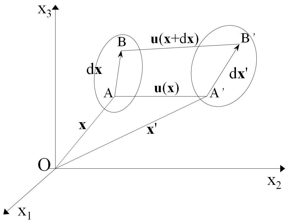
Figure 1 Schematic diagram of displacement and deformation of an infinitesimal line element in an elastic medium (adapted from Aki and Richards, 2002).

2.2 Staggered-grid finite-difference method

To solve the nonlinear wave equation (Eq. 9), we employ a high-accuracy Staggered-Grid Finite-Difference (SGFD) method (Virieux, 1986; Sun et al., 2018). First, by taking the time derivative of the nonlinear constitutive relation (Eq. 7) and combining it with the momentum conservation equation (Eq. 8), we convert the second-order wave equation into a system of first-order velocity-stress partial differential equations. This system includes additional stress-rate terms generated by the second-order products of displacement gradients. These terms update the displacement field through time integration of the velocity field, thereby implementing the nonlinear coupling. The resulting velocity-stress equations are:

$$\begin{array}{}\text{(10)}& \left\{\begin{array}{l}\mathit{\rho }\frac{\partial v_i}{\partial t}=\frac{\partial {\mathit{\sigma }}_{ij}}{\partial x_j}\\ \frac{\partial {\mathit{\sigma }}_{ij}}{\partial t}=\mathit{\lambda }{\mathit{\delta }}_{ij}\frac{\partial E_{kk}}{\partial t}+\mathrm{2}\mathit{\mu }\frac{\partial E_{ij}}{\partial t}\\ =\mathit{\lambda }{\mathit{\delta }}_{ij}\frac{\partial v_k}{\partial x_k}+\mathit{\mu }\left(\frac{\partial v_i}{\partial x_j}+\frac{\partial v_j}{\partial x_i}\right)\\ +\underset{\mathrm{additional}\mathrm{terms}}{\underbrace{\mathit{\lambda }{\mathit{\delta }}_{ij}\left(\frac{\partial v_k}{\partial x_m}\cdot \frac{\partial u_k}{\partial x_m}\right)+\mathrm{2}\mathit{\mu }\frac{\partial v_k}{\partial x_i}\cdot \frac{\partial u_k}{\partial x_j}}}\end{array}\right.,i,j,k,m\in \mathit{\{}x,y,z\mathit{\}}\end{array}$$

where $v_i=\partial u_i/\partial t$. In the SGFD scheme, different physical quantities are staggered on the spatial grid cells. This arrangement naturally satisfies the central-difference approximation for differential operators, effectively suppressing numerical dispersion and enhancing computational stability and accuracy, as illustrated in Fig. 2.

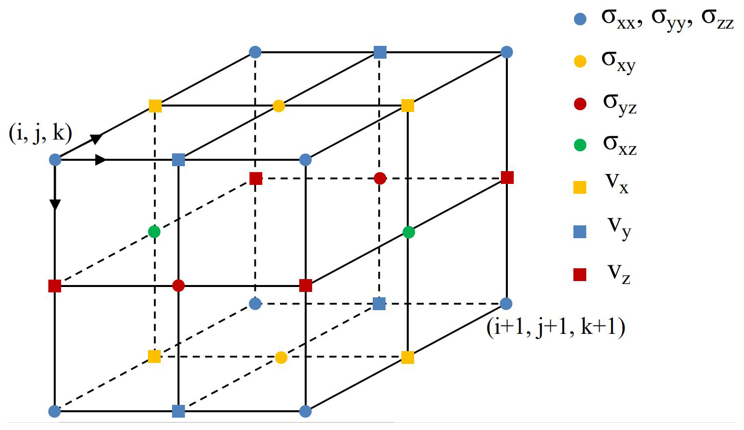
Figure 2 3D staggered-grid configuration for velocity-stress formulations, showing the placement of velocity components and stress components.

To handle the model's truncated boundaries, we employ the Perfectly Matched Layer (PML) absorbing boundary condition (Li et al., 2015). For simulations involving a free surface, the free boundary is implemented at the top of the model by setting the acoustic boundary replacement (Xu et al., 2007; Wang et al., 2012). The numerical code used in this study has been benchmarked against international standard programs, using SPICE/SISMOWINE. The comparison is provided in the supplementary material.

2.3 Source implementation and simulation parameters

The seismic moment tensor M_ij is the complete representation of an equivalent body-force system for a point source (Gilbert, 1970). It can be decomposed into three fundamental components: isotropy (ISO), double couple (DC), and compensated linear vector dipole (CLVD) (Knopoff and Randall, 1970; Jost and Hermann, 1989). These moment tensor expressions can be written as Eq. (11).

$$\begin{array}{}\text{(11)}& \begin{array}{rl}& M^{\mathrm{ISO}}=\left(\begin{array}{ccc}{M}_{xx}& \mathrm{0}& \mathrm{0}\\ \mathrm{0}& M_{yy}& \mathrm{0}\\ \mathrm{0}& \mathrm{0}& M_{zz}\end{array}\right),\\ & M^{\mathrm{DC}}=\left(\begin{array}{ccc}\mathrm{0}& M_{xy}& \mathrm{0}\\ M_{yx}& \mathrm{0}& \mathrm{0}\\ \mathrm{0}& \mathrm{0}& \mathrm{0}\end{array}\right),\\ & M^{\mathrm{CLVD}}=\left(\begin{array}{ccc}{M}_{xx}& \mathrm{0}& \mathrm{0}\\ \mathrm{0}& M_{yy}& \mathrm{0}\\ \mathrm{0}& \mathrm{0}& -\mathrm{2}{M}_{zz}\end{array}\right)\end{array}\end{array}$$

In our SGFD framework, we follow the method proposed by Graves (1996) to implement the moment tensor source by converting the moment rate tensor into equivalent body forces. The equivalent velocity increment Δvⁿ added on the grid can be expressed as:

$$\begin{array}{}\text{(12)}& {\displaystyle }{M}^{\mathrm{ISO}}:\mathrm{\Delta }{v}_i^n={\displaystyle \frac{M_{ij}\cdot dt\cdot f^n}{\mathit{\rho }V}}\cdot {\displaystyle \frac{\partial }{\partial x_j}}\text{(13)}& {\displaystyle }{M}^{\mathrm{DC}}:\mathrm{\Delta }{v}_i^n={\displaystyle \frac{M_{jk}\cdot dt\cdot f^n}{\mathit{\rho }V}}\cdot \left({\mathit{\delta }}_{ij}{\displaystyle \frac{\partial }{\partial x_k}}+{\mathit{\delta }}_{ik}{\displaystyle \frac{\partial }{\partial x_j}}\right)\text{(14)}& {\displaystyle }\begin{array}{rl}{M}^{\mathrm{CLVD}}:\mathrm{\Delta }{v}_i^n& ={\displaystyle \frac{M_{kl}\cdot dt\cdot f^n}{\mathit{\rho }V}}\cdot \left({\mathit{\delta }}_{ik}{\displaystyle \frac{\partial }{\partial x_l}}+{\mathit{\delta }}_{il}{\displaystyle \frac{\partial }{\partial x_k}}\right.\\ & \left.-{\displaystyle \frac{\mathrm{2}}{\mathrm{3}}}{\mathit{\delta }}_{kl}{\displaystyle \frac{\partial }{\partial x_i}}\right)\end{array}\end{array}$$

where i, j, k, $l\in \mathit{\{}x,y,z\mathit{\}}$. Δv is the velocity increment, n is the time-step index, dt is the time step, ρ is the density, V is the grid cell volume, and fⁿ is the value of the source-time function at time n⋅dt.

We conduct simulations in a homogeneous, isotropic, 3D full-space model to isolate the effects of nonlinearity from those of complex media. The model parameters are: P-wave velocity v_p=4400 m s⁻¹, S-wave velocity v_s=3000 m s⁻¹, and density ρ=2600 kg m⁻³. The model space is 14 km × 14 km × 14 km, with a uniform grid spacing of $\mathrm{\Delta }x=\mathrm{\Delta }y=\mathrm{\Delta }z=\mathrm{50}$ m. The source is located at the model center. It uses a Ricker wavelet with a dominant frequency of 4 Hz as the source-time function. Receivers are arranged on a spherical surface with a radius of 5 km centered at the source to sample wavefields at various azimuths. The time step is Δt=0.0015 s.

The shortest wavelength for the 4 Hz dominant frequency is the S-wavelength (λ_S=750 m). Based on the 50 m grid spacing, there are 15 grid points per wavelength, which is well above the threshold required for high-order finite-difference schemes (Virieux, 1986). The Courant–Friedrichs–Lewy (CFL) number is approximately 0.23, which is well below the stability limit for 3D finite-difference methods (Moczo et al., 2007), ensuring the stability and accuracy of the numerical computation.

3 Comparison of simulation results

3.1 Basic characteristics of nonlinear seismic wavefields

Figure 3a displays the 6C wavefield snapshots for the ISO source at t=1.5 s, while Fig. 3b compares the linear and nonlinear waveforms recorded at a specific receiver. Within the framework of linear theory, an ISO source only generates P-waves in homogeneous elastic media. However, a faint signal is still recorded in the P-wave window of the rotational components in the linear simulation (black line). This signal originates from the spatial gradients produced by the wavefront curvature of the near-field P-wave. In the far field, P-wave can be approximated as an irrotational plane wave with no curl in its displacement field. In the near field, however, the spatial gradients of its displacement field can generate weak rotation. This signal is very weak compared to the rotational signals generated by S-waves, and is therefore treated in this study as the baseline background for assessing the nonlinear contributions.

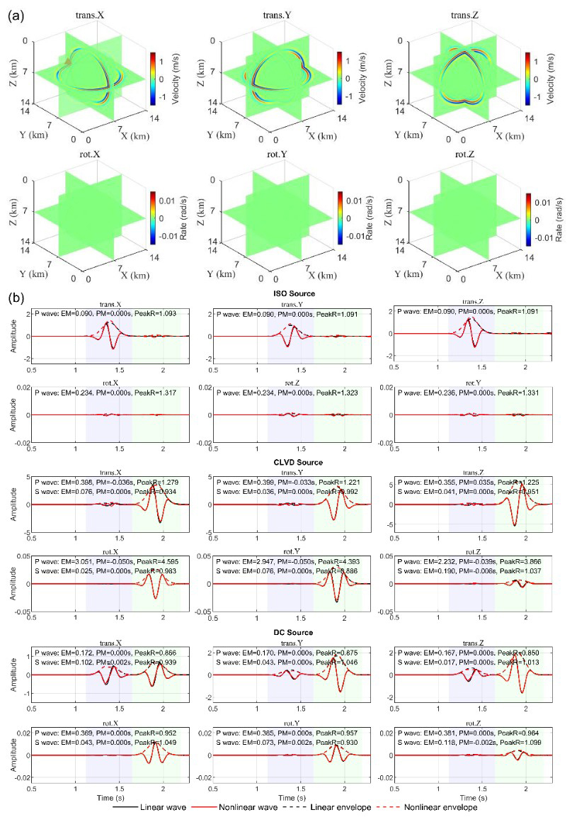
Figure 3 (a) Snapshot of the 6C wavefields from the linear ISO source simulation and the location of the example receiver (indicated by the red triangle on the trans.X component). (b) Comparison of the waveforms and envelope characteristics of the linear and nonlinear simulations at this receiver. The P-wave and S-wave analysis windows are marked. EM: envelope misfit; PM: phase misfit; PeakR: Peak ratio.

The waveform comparison shows that in the S-wave window, the nonlinear simulation exhibits a distinct response with obvious amplitude, whereas the linear simulation is near zero in the ISO results. This vibration is attributed to the P-to-S mode conversion of energy, caused by geometric nonlinearity. Analysis of the waveform characteristics in Fig. 3b reveals that the EM caused by nonlinearity is larger in the rotational components than in the translational ones, while the PM is nearly zero. This indicates that the primary effect of geometric nonlinearity is to modulate the energy distribution and envelope shape of the waves, rather than perturbing their fundamental propagation phase. This effect originates from the higher-order nonlinear terms in the strain-displacement relationship. These terms act as new, endogenous body force terms in the wave equation, equivalent to producing minor secondary perturbations in the wave's propagation. These perturbations interact with the primary wavefield, thereby reallocating energy and ultimately altering the wave's amplitude and shape. For instance, as a P-wave from an ISO source propagates, its non-uniform strain field generates spatial gradients. Through the self-interaction of these gradients via the nonlinear terms, an equivalent body force source with a curl component is generated within the medium, which then radiates S-waves.

We next calculated the energy of the residual waveforms between the linear and nonlinear simulations. Figure 4 shows the projection of this metric in the P-wave and S-wave windows onto three principal planes.

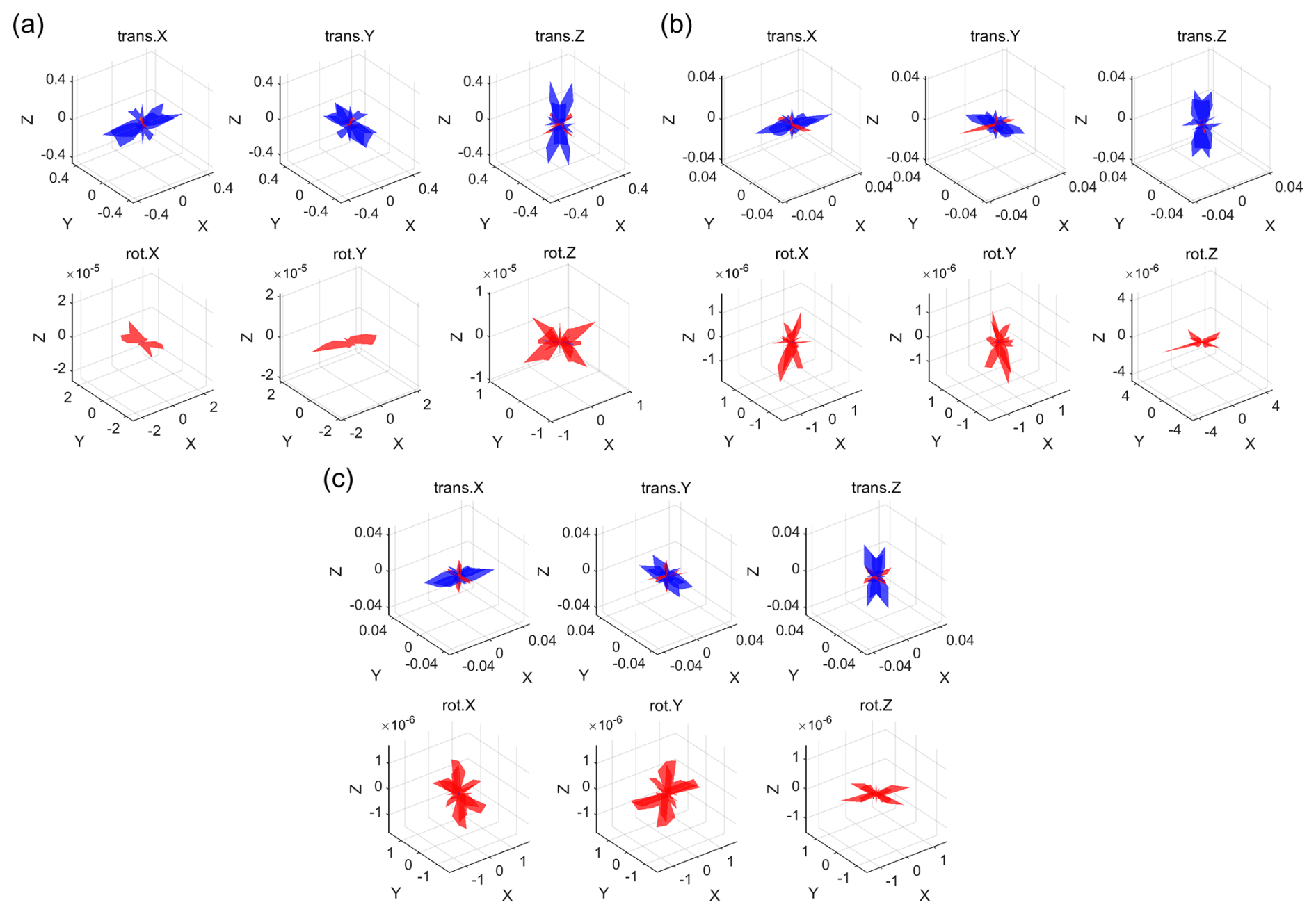
Figure 4 3D spatial projection of the intensity of waveform perturbations generated by nonlinearity. (a)–(c) are the results for CLVD, DC, and ISO sources, respectively. Each subplot shows the projection of the nonlinear effect intensity of the P-wave (blue) and the S-wave (red).

The results indicate that the radiation of the nonlinear effect follows fundamental wave physics principles. In the translational components, the nonlinear effect of the P-wave is much stronger than that of the S-wave, and its dominant direction is consistent with the corresponding coordinate axes, reflecting the direction of the strongest strain gradient in the linear P-wave field. Consequently, the nonlinear effect is strongest in the direction where the theoretical linear P-wave amplitude projects most strongly onto the corresponding Cartesian component (e.g., the x axis direction for the trans.X component). In the rotational components, the nonlinear perturbation in the S-wave is dominant. This is because rotational motion is generated by shear strain gradients, and the S-wave, carrying substantial shear energy, is most effective at producing the shear strain gradients required to drive rotation.

Building on the time-domain analysis, spectral analysis was conducted on waveforms in the P- and S-wave windows of the median and interquartile range (IQR) of the Power Spectral Density (PSD), as shown in Fig. 5. For the CLVD and DC sources, the median nonlinear spectrum is systematically higher than the median linear spectrum in the mid-to-high frequency band (approx. 5–20 Hz) in both P- and S-waves, and this phenomenon is more pronounced in the rotational components. The translational component spectra are nearly identical in the ISO source simulation. In the S-wave comparison for the ISO source, the linear translational and rotational energies are extremely low, essentially at the level of numerical simulation noise. In contrast, the nonlinear spectrum is several orders of magnitude higher, providing frequency-domain evidence for the nonlinear P–S mode conversion. The IQR of the PSD indicates that the nonlinear effects exhibit strong spatial variability, being enhanced in some azimuths while potentially being weakened in others, thus showing significant azimuthal dependence. The spectral comparison reveals a key feature of the nonlinear effect: energy transfer to higher frequencies. The energy injected by the source, primarily concentrated at lower frequencies, is efficiently pumped by the nonlinear secondary source and re-radiated as higher-frequency energy. This redistribution of high-frequency energy, accompanied by the mode conversion of P- and S-waves, collectively causes the nonlinear spectral lines to be systematically higher than the linear ones in the mid-to-high frequency range.

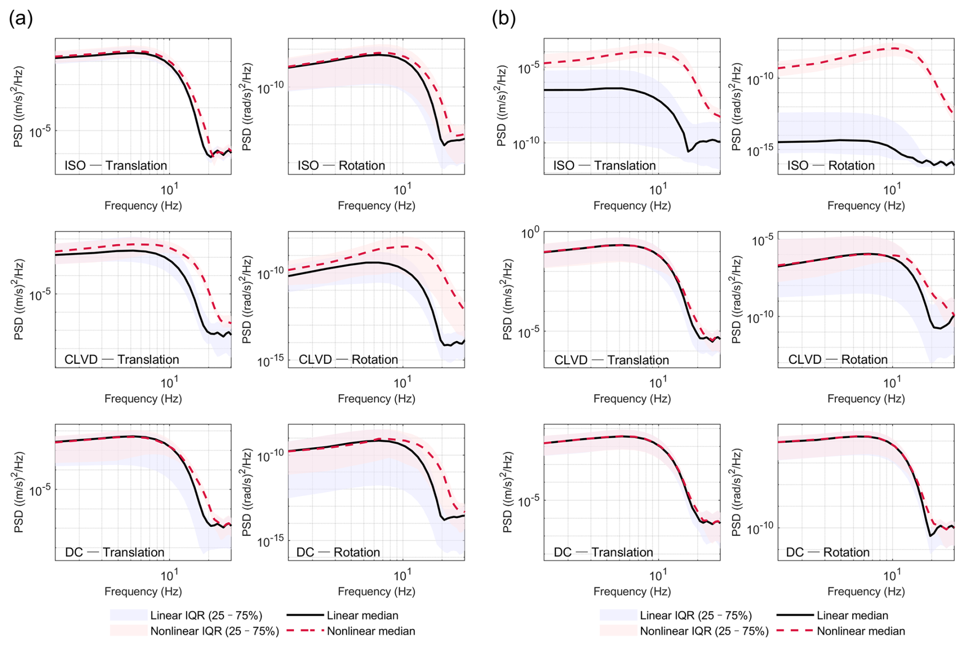
Figure 5 Comparison of the (a) P-wave and (b) S-wave PSD of translational and rotational components. The black solid line is the median PSD from the linear simulations, the red dashed line is from the nonlinear simulations, and the shaded area represents the 25 %–75 % IQR.

3.2 Source-type dependency of nonlinear effects

Figure 6 presents the log-ratio of nonlinear to linear energy ($\log (E_{\mathrm{nl}}/E_{\mathrm{lin}})$) for the tangential energy in the P-wave (E^P) and the radial energy in the S-wave (E^S). The energy E is obtained by time-integrating the square of the wavefield amplitude. Figure 6, through scatter plots and statistics, shows the distribution of the logarithmic energy ratios for the three source types, quantitatively assessing the overall impact of nonlinear effects on the energy of specific wave types.

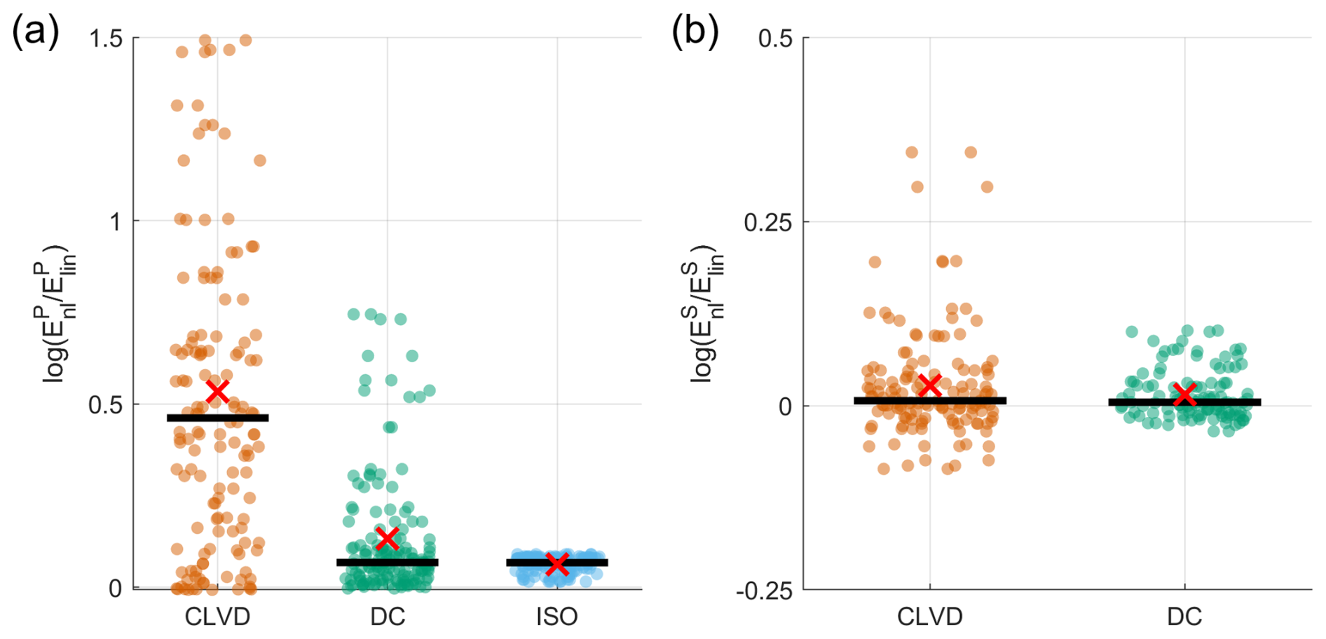
Figure 6 Distribution of the nonlinear/linear log-ratio for (a) tangential energy in the P-wave and (b) radial energy in the S-wave. The dots represent the values for each independent receiver; the black bar indicates the median of the data; the red cross indicates the arithmetic mean.

Regarding the tangential energy in the P-wave (Fig. 6a), the nonlinear enhancement is most significant for the CLVD source, followed by the DC source, while the effect of the ISO source is minimal. This indicates that the CLVD source is the most effective mechanism for exciting the nonlinear growth of P-wave tangential energy. For the radial energy in the S-wave (Fig. 6b), the net effect of nonlinearity for the CLVD and DC sources is not statistically significant, possibly due to the cancellation of azimuthal enhancement and reduction.

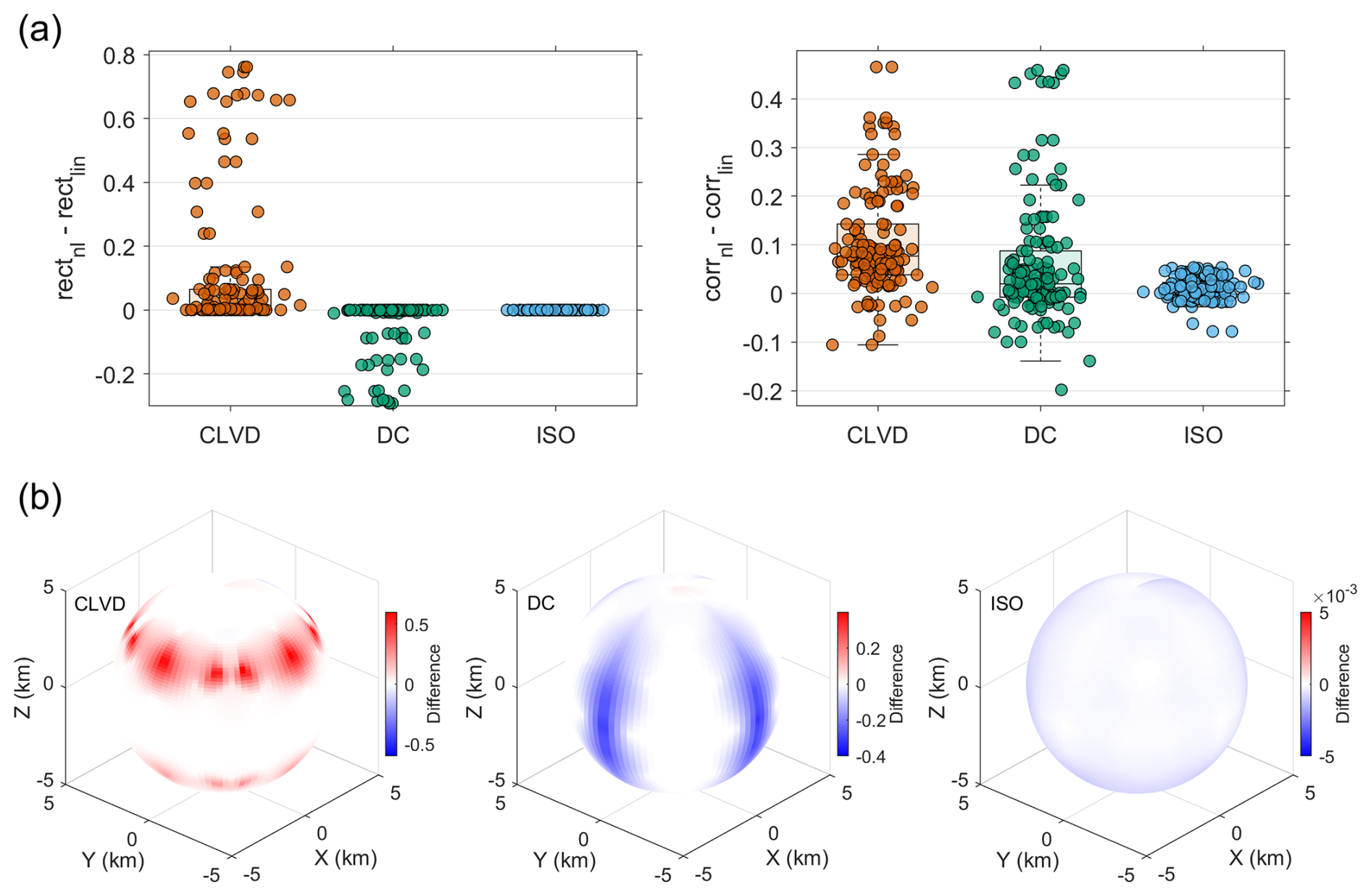
Figure 7 (a) Statistical distribution of the change in P-wave rectilinearity and rotation-translation correlation changes, and (b) spherical spatial distribution of Δ_rect in different receivers.

To further investigate the impact of nonlinearity on the micro-properties of the wavefield, we introduce two quantitative metrics to analyze the waveform attribute changes within the P-wave window. First, we use rectilinearity (rect) to measure the deviation of P-wave particle motion from a straight line. This metric is calculated based on the eigenvalues (${\mathit{\lambda }}_{\mathrm{1}}\ge {\mathit{\lambda }}_{\mathrm{2}}\ge {\mathit{\lambda }}_{\mathrm{3}}$) of the covariance matrix of the three-component particle motion data. While commonly defined as $-\mathrm{1}({\mathit{\lambda }}_{\mathrm{2}}+{\mathit{\lambda }}_{\mathrm{3}})/\mathrm{2}{\mathit{\lambda }}_{\mathrm{1}}$ (Jurkevics, 1988), we use a simplified and sensitive form, $\mathrm{rect}=({\mathit{\lambda }}_{\mathrm{1}}-{\mathit{\lambda }}_{\mathrm{2}})/{\mathit{\lambda }}_{\mathrm{1}}$. In this formulation, a value approaching 1 indicates purely unidirectional motion, whereas a value close to 0 indicates circular or random motion. The sign of the change, ${\mathrm{\Delta }}_{\mathrm{rect}}={\mathrm{rect}}_{\mathrm{nl}}-{\mathrm{rect}}_{\mathrm{lin}}$, reflects whether the nonlinearity promotes or suppresses the leakage of P-wave energy into the tangential direction. Second, to explore the coupling relationship between different motion modes, we introduce the rotation-translation correlation (corr). This metric is the Spearman's rank correlation coefficient between the time series of the tangential velocity magnitude and the rotation rate magnitude. This non-parametric metric was chosen to robustly quantify the synchrony of the time-varying intensity envelopes. It effectively assesses whether the two intensities trend together (i.e., a monotonic relationship), regardless of the specific functional form linking them (Press et al., 1986).

Figure 7a shows the statistical distribution of the differences in these two metrics. For all three sources, Δ_corr is generally positive, indicating that geometric nonlinearity may be a common physical mechanism that enhances the coupling between rotation and translation. In contrast, the distribution of Δ_rect shows a pronounced source dependence: the ISO source causes weak changes, the DC source induces significant negative changes, while the CLVD source primarily causes positive changes. The spatial distribution of Δ_rect in Fig. 7b further reveals its essential connection to the source's strain state. For the ISO source, characterized by pure volumetric strain, the pure volumetric strain excites a very weak shear effect through nonlinearity, leading to a slight decrease in P-wave rectilinearity, but the efficiency of this conversion is extremely low. For the pure-shear DC source, the significant decrease in rectilinearity is concentrated near the P-wave radiation nodes, which are the regions with the strongest linear shear strain gradients. This indicates that in these regions, the efficiency of the nonlinear P–S mode conversion is highest, leading to a noticeable decrease in rectilinearity. For the CLVD source, which combines strong uniaxial compression and axisymmetric shear, the increase in rectilinearity is also concentrated in regions with strong strain gradients. The result reveals that, in a complex stress state with coexisting tension and compression, the nonlinear effect may instead constrain energy to propagate in the radial direction, suppressing leakage into the tangential direction, thereby purifying the P-wave motion.

In summary, the analysis of the wavefield properties demonstrates that the manifestation of nonlinear effects is fundamentally controlled by the type of strain field initialized by the source and the geometry of its spatial gradients. Different source mechanisms, by initializing different strain fields, thus modulate the mode, intensity, and even the effect of the nonlinear response.

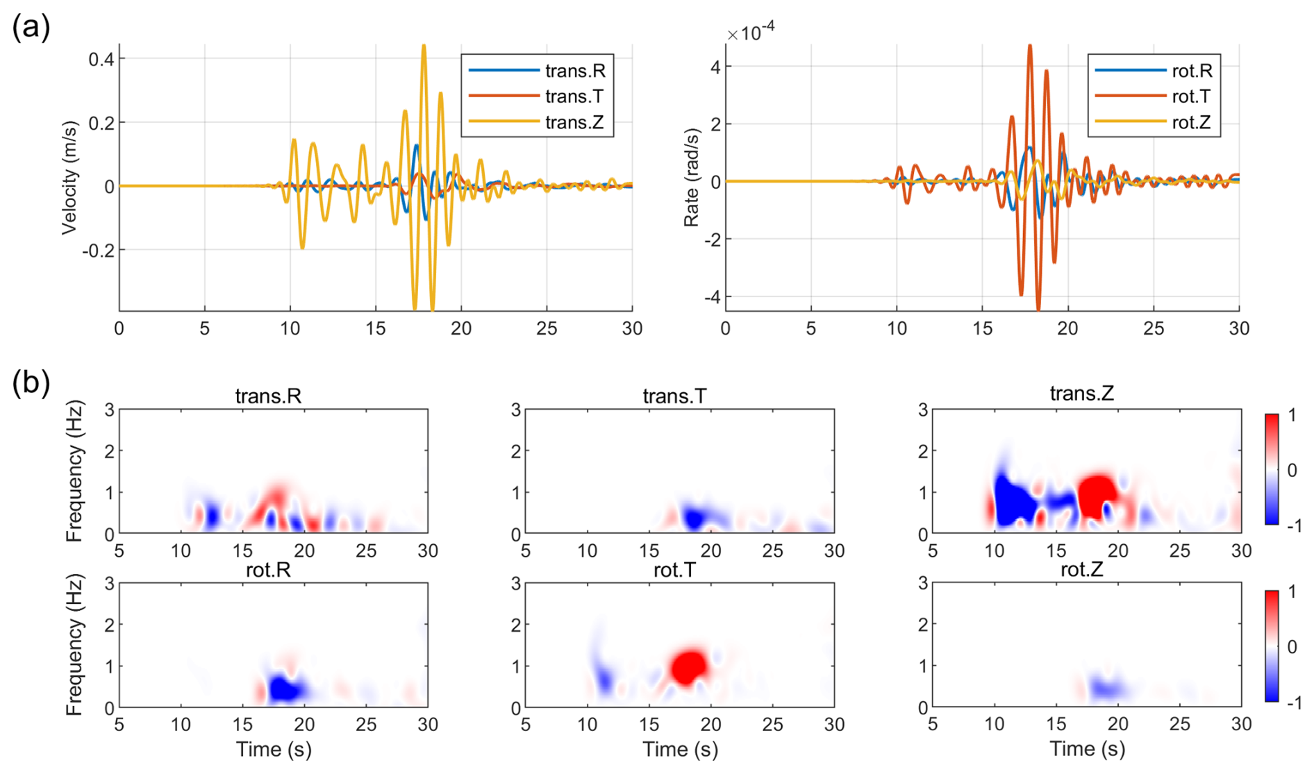
Figure 8 (a) Synthetic linear 6C waveforms (low-pass filtered at 2 Hz) and (b) normalized time-frequency spectral differences (the nonlinear minus the linear) for event E1.

4 Simulation of nonlinear effects for referenced earthquake events

To extend the understanding established in the idealized full-space model to more realistic scenarios involving complex propagation effects, we further simulate two moderate-to-strong referenced earthquakes that occurred in the coastal region of Taiwan: event E1 (M_w 5.4) and event E2 (M_w 6.1). The epicenters and station locations of these two referenced events are shown in Fig. S3. Unlike the preceding basic source simulations, the models in this section employ a layered velocity structure based on the CRUST1.0 model (Laske et al., 2013) to approximate the real Earth's structure (see Table S4). The source mechanisms for both events (Eq. 13) are composite, containing both non-double-couple and double-couple components. Other detailed simulation parameters for the two referenced earthquake simulations are provided in Table S5.

$$\begin{array}{}\text{(15)}& \begin{array}{l}\mathrm{E}\mathrm{1}:\left[\begin{array}{lll}{M}_{xx}=-\mathrm{7.569}\times {\mathrm{10}}^{\mathrm{16}},& M_{yy}=-\mathrm{2.373}\times {\mathrm{10}}^{\mathrm{16}},& M_{zz}=\mathrm{9.942}\times {\mathrm{10}}^{\mathrm{16}}\\ M_{xz}=\mathrm{7.372}\times {\mathrm{10}}^{\mathrm{16}},& M_{yz}=-\mathrm{1.0965}\times {\mathrm{10}}^{\mathrm{17}},& M_{xy}=\mathrm{4.156}\times {\mathrm{10}}^{\mathrm{16}}\end{array}\right.\\ \mathrm{E}\mathrm{2}:\left[\begin{array}{lll}{M}_{xx}=-\mathrm{1.064}\times {\mathrm{10}}^{\mathrm{18}},& M_{yy}=-\mathrm{7.607}\times {\mathrm{10}}^{\mathrm{17}},& M_{zz}=\mathrm{1.8247}\times {\mathrm{10}}^{\mathrm{18}}\\ M_{xz}=\mathrm{3.141}\times {\mathrm{10}}^{\mathrm{17}},& M_{yz}=\mathrm{3.155}\times {\mathrm{10}}^{\mathrm{17}},& M_{xy}=\mathrm{1.114}\times {\mathrm{10}}^{\mathrm{18}}.\end{array}\right.\end{array}\end{array}$$

Figure 8 shows the results for the E1. Compare the waveforms and the time-frequency spectral differences, where the spectra are calculated using a Generalized S-Transform (GST) (Stockwell et al., 1996), as shown in Fig. 8b. These differences are defined as the spectra of the nonlinear simulations minus those of the linear simulations. In the translational components, the energy changes induced by nonlinearity are relatively dispersed in different types of waves. However, most are concentrated during the arrival of S-wave (approx. 15–20 s) and the subsequent surface waves, and faint but persistent nonlinear perturbations are also observed during the P-wave and its subsequent multiple reflections/conversions (approx. 5–15 s). In the rotational components, the nonlinear response energy is more concentrated than in the translational components. Energy perturbations can be observed on the rot.T component before the direct S-wave arrival, which may correspond to nonlinear effects excited by S-waves converted from P-waves or S-waves reflected/transmitted within the layered medium. For the rot.R and rot.Z components, the nonlinear effects are primarily associated with the arrival of the direct S-wave. Different components showing different extents of nonlinearity may stem from the azimuthal location of this receiver.

Numerical simulations of the E2 (Fig. 9) also show nonlinear effects. Combining the time-domain waveforms (Fig. 9a) and the time-frequency spectral energy difference plots (Fig. 9b), it can be seen that significant energy changes occur in all components during the arrival of the direct S-wave (approx. 90 s) and the strong surface waves. A long-duration, very-low-frequency (<0.2 Hz) energy enhancement band appears in the translational components, starting from the surface waves and continuing. This may correspond to long-period perturbations induced by strong surface waves through nonlinear mechanisms, potentially involving P–S coupling in layered media, while the rotational components, as displacement gradients, are not sensitive to it.

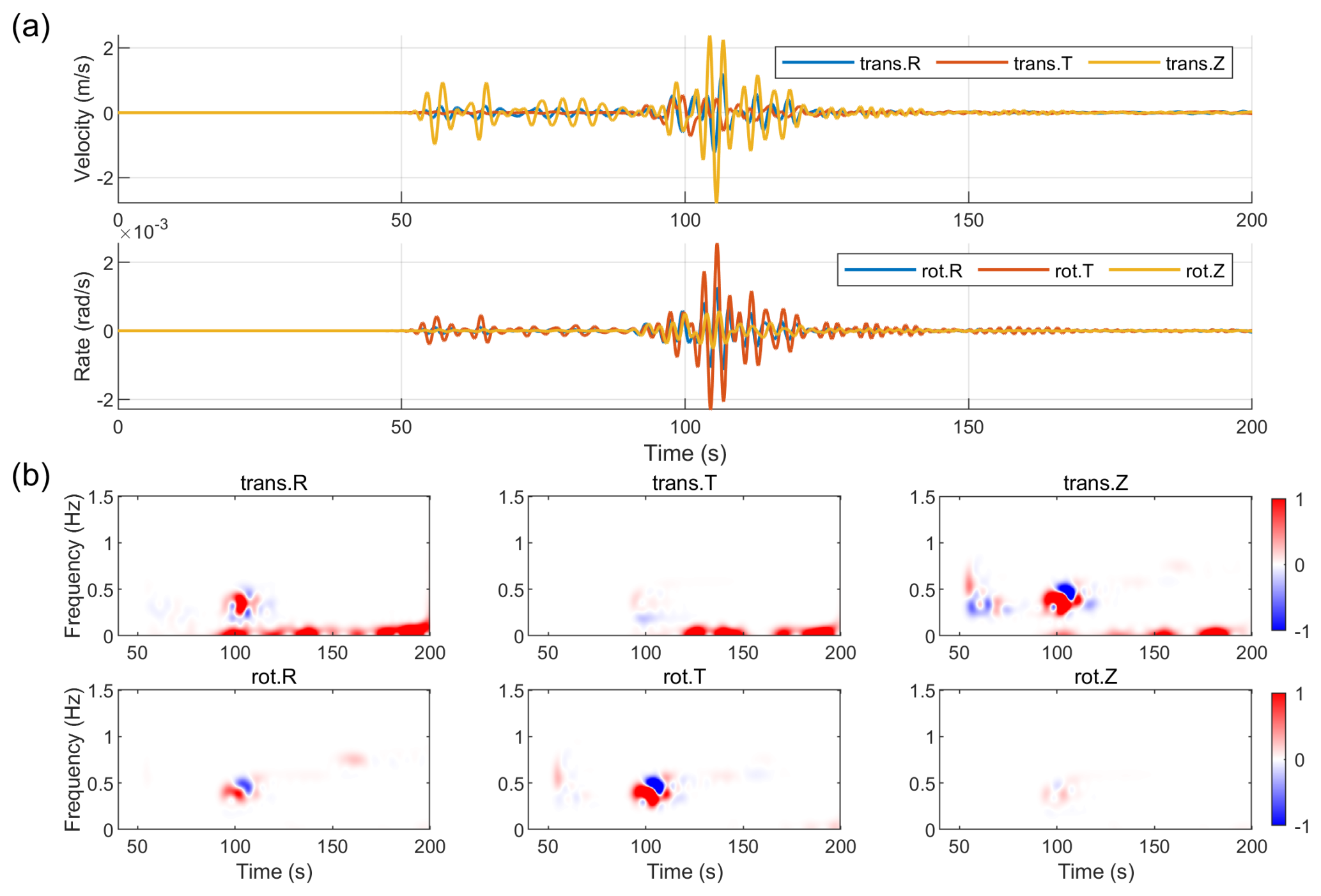
Figure 9 (a) Synthetic linear 6C waveforms (low-pass filtered at 1 Hz) and (b) normalized time-frequency spectral differences (the nonlinear minus the linear) for event E2.

By comparing the simulations of the two events, we find that the surface waves are the primary phases that accumulate and carry nonlinear information. At the same time, the E2 event, with its different source mechanism and further propagation path, exhibits a long-period perturbation not seen in the E1 simulation. This suggests that in more realistic scenarios, the physical mechanisms of nonlinear effects may be more complex and can be influenced by many factors. The different nonlinear characteristics displayed by the two event simulations may also be influenced by the combined effects of their complex, composite source mechanisms and the specific source-station azimuth.

5 Discussion

This study, through systematic simulations of three basic moment-tensor source types and referenced earthquake events, has demonstrated several characteristics of geometric nonlinearity in seismic wavefields. First, it demonstrates that the excitation and manifestation of nonlinear effects are controlled by the strain state of the linear wavefield and its spatial gradients. As predicted by nonlinear elastodynamic theory, geometric nonlinearity acts as an equivalent secondary source term in the wave equation, with its strength being proportional to the quadratic terms of the linear strain field. The radiation of nonlinear effects strictly follows the physical nature of longitudinal and transverse waves. For instance, the nonlinear perturbation generated by the strain gradients of a linear P-wave radiates most strongly along the principal direction of the P-wave, whereas the nonlinear rotational effect generated by the shear-strain gradients of an S-wave is most pronounced in regions of maximum S-wave energy. In addition, different source mechanisms (volumetric, pure shear, axisymmetric shear) modulate the mode, strength, and even the effect of the nonlinear response by initializing different geometries of the strain field.

Second, rotational motion is a sensitive indicator for detecting near-field nonlinear effects driven by S-waves. This stems from the physical nature of rotation – it is the spatial gradient of the displacement field and is therefore more sensitive to the secondary source terms driven by strain gradients. This suggests that the deployment and analysis of six-component seismic data are of irreplaceable value for identifying and quantifying nonlinear geophysical processes in future observational studies.

Finally, the simulations of referenced earthquake events show that surface waves, which are more concentrated in energy and have longer propagation paths, are the primary carriers for accumulating and preserving nonlinear information, thus pointing to a key focus for future observational data analysis. More importantly, in the stronger E2 event, we observed a long-period perturbation not seen in the idealized models. This phenomenon suggests that under realistic strong ground motion conditions, the physical mechanisms of nonlinear effects may be more complex and diverse, potentially involving deeper physical processes such as stress-induced anisotropy. Limitations of this study, such as the use of idealized models, highlight the need for validation with real seismic records. These indicate a direction for future research: how to reliably separate and identify these unique nonlinear signals from collected real seismic records, which is a mixture of complex source effects, 3D heterogeneous propagation effects, and local site responses.

6 Conclusions

By incorporating geometric nonlinearity based on the Green–Lagrange strain tensor, this study has conducted 6C seismic wavefield simulations for three fundamental moment tensor sources and two referenced moderate-to-strong earthquakes. The research aims to investigate the characteristics of near-field nonlinear effects and their dependence on source mechanisms. The main conclusions are as follows:

• i.

  Universal radiation pattern of the nonlinear secondary source and source-dependent efficiency of exciting the effects. On one hand, the radiation pattern of nonlinearity is universal, strictly adhering to the physics of wave motion: the nonlinear perturbation generated by P-wave strain gradients radiates primarily along the axial direction (a longitudinal characteristic), while the perturbation from S-wave shear-strain gradients radiates mainly in the orthogonal plane directions (a transverse characteristic). This pattern is independent of the initial force source type. On the other hand, the overall efficiency of exciting these nonlinear secondary sources exhibits a strong source-type dependency. Simulation results show that sources with significant shear components, such as CLVD and DC sources, are far more efficient in exciting nonlinear effects than the purely volumetric ISO source.

• ii.

  High sensitivity of rotational motion to S-wave-driven nonlinearity. This is primarily because rotational motion directly responds to shear-strain gradients, and S-waves are the primary carriers of shear energy. Consequently, rotational motion becomes an ideal window for detecting the secondary sources excited by S-waves, with its nonlinear response being more pronounced than that of translational components.

• iii.

  Effects of wave type and strain level. The strength of nonlinear effects is correlated with the strain level (which can be approximately related to the moment magnitude). More importantly, surface waves, which have more concentrated energy and longer propagation paths, are more effective carriers of nonlinear information than body waves. In the strong-motion event simulation, long-period perturbations, possibly induced by nonlinearity, were also observed. This may correspond to long-period perturbations induced by strong surface waves through nonlinear mechanisms, potentially involving P–S coupling in layered media.