Multifractal analysis of wind turbine power and rainfall from an operational wind farm – Part 2: Joint analysis of available wind power and rain intensity

In the increasing global transition towards renewable and carbon-neutral energy, understanding the uncertainties associated with wind power production is extremely important. In addition to the widely acknowledged uncertainties from turbulence and wind intermittency, further complexity arises from the influence of rainfall, which only a limited number of studies have addressed so far. To understand this, multiple 3D sonic anemometers, mini meteorological stations, and optical disdrometers were employed on a meteorological mast on the Pays d'Othe wind farm (110 km south-east of Paris, France) in the framework of the Rainfall Wind Turbine or Turbulence (RW-Turb) project (https://hmco.enpc.fr/portfolio-archive/rw-turb/, last access: 26 November 2024). With these simultaneously measured data, wind power and its associated atmospheric fields were studied under various rainy conditions.

Variations of the wind velocity, power available on the wind farm, power produced by wind turbines, and air density are examined here, under rainy and dry conditions, using the scale-invariant framework of universal multifractals (UM). Since rated power acts like an upper threshold in statistical analysis of turbine power (discussed in Part 1), theoretically available power was used as a proxy. From an event-based analysis, differences in UM parameters were observed between rainy and dry conditions for the fields. This is explored further using joint multifractal analysis, which revealed an increase in the correlation exponent between various fields with the rain rate. Here we also examine the possibility of variation in power production by rainy conditions (convective or stratiform) as well as by regimes of wind velocity. While examining time steps according to wind velocity, turbine power curves showed different regions of departure from the state curve according to the rain rate.

1 Introduction

Wind energy is seen as the forerunner in the renewable energy sector, whose rapid growth (4 times greater than the current rate) is highly desirable for a sustainable future (where 57 % of the global power supply is renewable by 2030, up from 26 % in 2019), which ensures climate protection (IRENA, 2020). Wind power production also plays an important role in achieving United Nations Sustainable Development Goal (SDG) 7 – affordable and clean energy for all. According to the IEA (2020) wind overview, global wind power capacity has increased by 14 %, with annual installations increasing by 54 % or 60 GW. This is projected to increase as the UN high-level Dialogue on Energy in 2021 (UN, 2022) called for global doubling of annual investment in renewable energy and energy efficiency by 2025 (triple by 2030, creating 60 million jobs worldwide).

Modern wind turbines extract power from wind in the atmosphere and convert it into electricity, which can be stored and distributed to locations of use via power grids. The popularly known term “windmill” refers to the historic usage where wind power was converted to mechanical energy at the location of the usage (Manwell et al., 2010). According to WindEurope (previously EWEA), an average offshore wind turbine (of capacity 2.5–3 MW; the Vestas V-90 used in this study falls into this category) can produce more than 6 million kilowatt hours a year, which is enough for 1500 average EU households. As per their estimation, by 2050, wind power production is expected to meet 50 % of the European Union's energy demands (EWEA, 2012). In the context of France, wind alone accounts for one-third of the total renewable power production in 2021 (Jørgensen and Holttinen, 2022), which is set to increase as the country aims to have 50 offshore wind farms by 2050 through simplified legislation (Engie, 2022). One of the results from the Cai and Bréon (2021) evaluation of wind power potential in France is that climate change will not significantly impact the statistical properties of the mean load factor, thus making wind a reliable energy source in these changing times.

Small-scale fluctuations and intermittence in wind make their characterization difficult as a field, which in turn shows further spatio-temporal variability. This and the atmospheric turbulence (more complicated owing to the hub location near the boundary layer) are transferred to the power produced. To account for this, a common practice is to use a coarser parameter such as turbulent intensity (standard deviation of wind speed divided by mean wind speed over 10 min), which does not capture the above complexities at smaller scales or affect external turbulent factors such as rain (Johnson, 2004). Only a limited number of studies have tried to address the effect of rain on power production so far. An earlier study by Corrigan and Demiglio (1985) reported a reduction in power production (20 % to 30 %, using a 38 m diameter two-blade turbine); this was later confirmed experimentally (Al et al., 1986). Cohan and Arastoopour (2016) (improving upon Cai et al., 2013) examined the effect of rain on a wind turbine blade aerofoil using multi-phase (air as volatile and rain as liquid) computational fluid dynamics (CFDs) and reported high sensitivity to performance at lower rain rates till a rain rate is high enough to immerse most of the aerofoil surface underwater. Some positive influence of rain was also reported, such as cleaning of blades (Corten and Veldkamp, 2001), increasing power production. Rain can also have long-term effects as the kinetic energy of impacting raindrops can cause leading-edge erosion (LEE) on turbine blades, reducing their aerodynamic performance; this in turn results in lower annual energy and increased downtime (Keegan et al., 2013).

It is hence of interest to quantify the effect of rainfall on wind power (theoretically available and operationally measured). The widely used scale-invariant framework of universal multifractals (UM) is of interest for characterizing wind and its correlation with other atmospheric fields (Schertzer and Lovejoy, 1987). See also Appendix A of the companion paper (Jose et al., 2024) for a comparison with the other formalisms. Calif and Schmitt (2014) illustrated the intermittent and multifractal nature of turbulent wind speed and aggregate power from a wind farm over a wide range of scales and showed coupling with a generalized correlation function (GCF)-based joint multifractal description (Meneveau et al., 1990). The specific framework of UM was used previously (Fitton et al., 2011, 2014) to study the scaling behaviour and multifractal properties of wind velocity and torque fluctuations. Here, continuous high-resolution (100 Hz) measurements of 3D wind velocity along with other atmospheric fields (and rain) from a meteorological mast located on a functional wind farm (Gires et al., 2022) were subjected to multifractal analysis in a two-fold analysis. The first part consisted of multifractal characterization of the fields using UM; this was followed by characterization of the correlation using joint multifractal analysis (JMF), which is derived from UM (Gires et al., 2020a).

Details of the data collection and quality are presented in the second part of the upcoming section on data and methods; the first part of this section briefly recapitulates the frameworks of UM and JMF. In the first part of Sect. 3, individual UM analyses of fields are presented along with the biases encountered. In the second part of Sect. 3, various fields are analysed jointly (using JMF), and the correlations obtained between the various fields are discussed along with possible biases. In Sect. 4, the influences of rain type and wind direction on power production are discussed. Section 5 concludes the study and summarizes the results.

2 Methodology and data

2.1 Scaling analysis and UM framework

Spectral analysis is widely used for characterizing scaling properties. Here, the second-order statistics of rain in the frequency domain were examined for power-law scaling as follows (Mandelbrot, 1982; Schertzer and Lovejoy, 1983):

$$\begin{array}{}\text{(1)}& E\left(k\right)\approx k^{-\mathit{\beta }},\end{array}$$

where k corresponds to the wave number and β is the spectral exponent.

However, to fully characterize the complexity of the process across its intensities and spatio-temporal variations, information on higher- and lower-order statistics is required. For this, we use UM, which rely on the assumption of the field being generated by an underlying cascade process with conserved statistical properties at each scale while inheriting the scale-invariant properties of Navier–Stokes equations (Schertzer and Lovejoy, 1987, 1989; Schertzer and Tchiguirinskaia, 2020). In this framework, the probability of a field exceeding a particular threshold across all the scales is captured using the scale-invariant notion of singularity (γ), and for a multifractal field this scales according to the resolution ($\mathit{\lambda }=L/l$, i.e. the ratio of L, the outer scale, to l, the observational scale) with the corresponding fractal co-dimension as the scaling exponent c(γ) (Schertzer and Lovejoy, 1987, 1988):

$$\begin{array}{}\text{(2)}& p({\mathit{ϵ}}_{\mathit{\lambda }}\ge {\mathit{\lambda }}^{\mathit{\gamma }})\approx {\mathit{\lambda }}^{-c\left(\mathit{\gamma }\right)}.\end{array}$$

This relation implies that statistical moments q of the field scale with the resolution of the moment-scaling function K(q) as (Schertzer and Lovejoy, 1987, 1988)

$$\begin{array}{}\text{(3)}& \langle {{\mathit{ϵ}}_{\mathit{\lambda }}}^q\rangle \approx {\mathit{\lambda }}^{K\left(q\right)}.\end{array}$$

K(q) and c(γ) are equivalent functions related through Legendre transform (Parisi and Frisch, 1985), and they fully characterize the variability of the field across all the scales. For a conservative field in the UM framework, K_c(q) can be fully determined with the help of only two parameters with physical interpretation, a multifractal index α, and a mean intermittency co-dimension C₁ (Schertzer and Lovejoy, 1987, 1988). This yields

$$\begin{array}{}\text{(4)}& K_{\mathrm{c}}\left(q\right)=\left\{\begin{array}{ll}{\displaystyle \frac{C_{\mathrm{1}}}{\mathit{\alpha }-\mathrm{1}}}(q^{\mathit{\alpha }}-q)& \mathit{\alpha }\ne \mathrm{1},\\ C_{\mathrm{1}}q\ln q& \mathit{\alpha }=\mathrm{1}.\end{array}\right.\end{array}$$

C₁ measures clustering of the average intensity across scales ($C_{\mathrm{1}}\in [\mathrm{0},\mathrm{1}]$ for one-dimensional fields): when C₁=0, the field is homogeneous with little variability. α measures how this clustering changes with respect to intensity levels ($\mathit{\alpha }\in [\mathrm{0},\mathrm{2}]$): the higher the value of α, the higher the variability, with α=0 being a mono-fractal field where intermittency of the extreme is the same as that of the mean.

For a non-conservative field ψ_λ, i.e. a field whose average (〈ψ_λ〉) changes with scales, a non-conservative parameter H is used in the expression of scaling (Schertzer and Lovejoy, 1987, 1988):

$$\begin{array}{}\text{(5)}& {\mathit{\psi }}_{\mathit{\lambda }}{=}^{\mathrm{d}}{\mathit{ϵ}}_{\mathit{\lambda }}{\mathit{\lambda }}^{-H},\end{array}$$

where =^d denotes the equality in the distribution ($X{=}^{\mathrm{d}}Y\iff \forall x:\text{Pr}(X>x)=\text{Pr}(Y>x)$) and ϵ is a conservative field characterized by C₁ and α. For a conservative field, H = 0. For a non-conservative field with a positive value of H, fractional differentiation is required to retrieve a conservative field. Similarly, for a non-conservative field with a negative value of H, the conservative field is retrieved through fractional integration. H is related to the spectral slope β (Eq. 1) as (Tessier et al., 1993)

$$\begin{array}{}\text{(6)}& \mathit{\beta }=\mathrm{1}+\mathrm{2}H-K_{\mathrm{c}}\left(\mathrm{2}\right).\end{array}$$

The scaling behaviour of conservative multifractal fields can be examined using a trace moment (TM) where a log–log plot of upscaled fields against a resolution λ is taken for each moment q (Eq. 3). The quality of scaling is given by the estimate r² of the linear regression; the value for q=1.5 is used as a reference. A double trace moment (DTM) is a more robust version of a TM tailored for UM fields, where the moment-scaling function K(q,η) of the field ${{\mathit{ϵ}}_{\mathit{\lambda }}}^{\left(\mathit{\eta }\right)}$ (a field raised to power η at maximum resolution and re-normalized) is expressed as a function of the multifractal index α (Lavallée et al., 1993):

$$\begin{array}{}\text{(7)}& \langle ({{\mathit{ϵ}}_{\mathit{\lambda }}}^{\left(\mathit{\eta }\right)}{)}^q\rangle \approx {\mathit{\lambda }}^{K(q,\mathit{\eta })}={\mathit{\lambda }}^{{\mathit{\eta }}^{\mathit{\alpha }}K\left(q\right)}.\end{array}$$

From the above equation, the value of α can be obtained as the slope of the linear part when K(q,η) is represented for a given q as a function of η in a log–log plot. Both the TM and DTM techniques give reliable estimates as long as H is less than 0.5 for the field analysed.

Since multifractal processes are generated by cascade processes, the average values can become too concentrated over a certain area, leading to spurious estimates of moments above a particular value of q (at q_D, q is above $K\left(q\right)\approx +\mathrm{\infty }$), which is a divergence of moments. The functions K(q) and c(γ) are also limited by the sample size of the data or rather the maximum value of the scale-invariant threshold or singularity (γ_s) and the corresponding moment (q_s). For reliable statistical estimates of the moment-scaling function and hence the UM parameters, the moment orders should not exceed q_s or q_D.

2.2 Framework of JMF

Though not extensive, various methodologies were suggested and used for studying coupling (across scales) between two simultaneously measured fields from their joint moments (like the moments of the individual fields mentioned before but by multiplying both fields under consideration). Schertzer and Tchiguirinskaia (2020), and the references therein considered multivariate multifractals. Meneveau et al. (1990) used joint moment exponents to examine the correlation between velocity and temperature fluctuations in the turbulent wake of a heated cylinder and between the square of vorticity fluctuations and the dissipation of a turbulent velocity component. Seuront and Schmitt (2005a, b) expanded on this by introducing a GCF (re-normalizing the joint moments) and argued for the use case by effectively characterizing biological and physical coupling (using data on phytoplankton concentration, fluorescence, and temperature at various turbulence intensities). Calif and Schmitt (2014) used GCFs to examine coupling between simultaneous data of wind speed and the aggregate power output from a wind farm. Both cases used GCFs on log-normal cascades involving single-parameter and linear correlation functions and explored only two specific coupling cases between fields – a proportional relation or a power law relation. Between the two fields, the GCF is symmetrical with respect to the moment between them; this suggests the possibility of expressing the two quantities with a simple relation of proportionality. Relying on this, Gires et al. (2020a) expanded GCFs to UM by providing a framework (JMF) where related fields can be expressed as a multiplicative power law combination of known UM fields. This framework not only retrieves the proportionality constants between fields but also provides an intuitive indicator that combines most of the information obtained from JMF.

Consider two simultaneously measured multifractal fields ϵ_λ and ϕ_λ of resolution λ. In JMF, we can express ϵ_λ in terms of ϕ_λ and an independent multifractal field Y_λ with the same C₁ as ϕ_λ. Below, both fields are correlated with a and b (relative weight in combination), and Y_λ can be generated if we know its α and C₁. Note that ${{\mathit{\varphi }}_{\mathit{\lambda }}}^a{Y_{\mathit{\lambda }}}^b$ is a single field expressed as a power law combination of ϕ and Y:

$$\begin{array}{}\text{(8)}& {\mathit{ϵ}}_{\mathit{\lambda }}={\displaystyle \frac{{{\mathit{\varphi }}_{\mathit{\lambda }}}^a{Y_{\mathit{\lambda }}}^b}{\langle {{\mathit{\varphi }}_{\mathit{\lambda }}}^a{Y_{\mathit{\lambda }}}^b\rangle }}.\end{array}$$

Before proceeding further, it is important to state the meaning of a and b intuitively for correlation between fields. When a=1 and b=0, ϵ_λ is simply equal to ϕ_λ (maximum correlation), and during the converse ϵ_λ is equal to Y_λ with no connection to ϕ_λ. Intermediate values of a ($\mathrm{1}>a>\mathrm{0}$) show progressive decorrelation between ϵ_λ and ϕ_λ. With a, b, and Y_λ, it is possible to characterize the correlation between two multifractal fields. Along with these parameters, the JMF framework also introduces a simplified indicator of correlation, IC_ϵϕ (≈IC_ϕϵ):

$$\begin{array}{}\text{(9)}& {\mathrm{IC}}_{\mathit{ϵ}\mathit{\varphi }}={\displaystyle \frac{C_{\mathrm{1},\mathit{\varphi }}{a}^{{\mathit{\alpha }}_{\mathit{\varphi }}}}{C_{\mathrm{1},\mathit{ϵ}}}}.\end{array}$$

More information on the intuitive indicator and exponents can be found in Gires et al. (2020a), along with a validation of the framework with real and simulated data and a discussion of some of the limitations. The IC is reported to be relevant for values of α typically greater than 0.8, which is the case for the field studied here.

2.3 Instrumentation, data, and biases

2.3.1 Instrumentation and directly measured fields

As discussed, understanding the long-term and short-term effects of rainfall on wind power production is important, and the Rainfall Wind Turbine or Turbulence project (RW-Turb; https://hmco.enpc.fr/portfolio-archive/rw-turb/, last access: 26 november 2024), supported by the Agence Nationale de la Recherche (ANR, French National Research Agency in English), is designed to address this with simultaneous real-time in situ measurements of rain and wind at the turbine's location. To recap, the RW-Turb measurement campaign (Pay d'Othe, 110 km south-east of Paris, France) consists of a meteorological mast on an operational wind farm (jointly operated by Boralex and JP Énergie Environnement), with two sets of optical disdrometers (OTT Parsivel²), 3D sonic anemometers (ThiesCLIMA), and a mini meteorological station at heights of roughly 45 and 80 m. The finest available measurement time steps are 30, 0.01, and 1 s respectively. Figure 1 briefly summarizes the instrumentation and location of the meteorological mast.

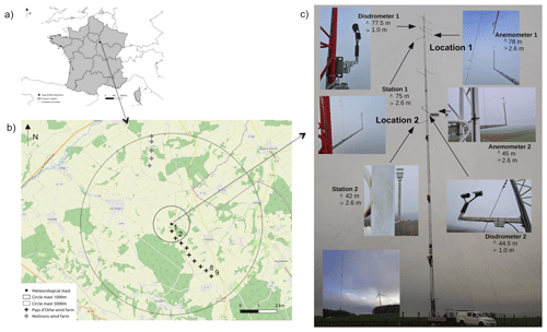
Figure 1 (a) Location of the Pays d'Othe wind farm in France. (b) Map of the surroundings: the meteorological mast is in the centre, and the available turbines are numbered 1, 2, 8, and 9. (c) Summary of the measurement devices on the meteorological mast and their vertical locations. Figures adapted from Gires et al. (2022).

Interested readers are directed to Gires et al. (2022) for an overview of the campaign with data and instrumentation; a 3-month-long dataset is also made publicly available there along with the raw files and scripts required for their usage. The actual sampling rates are discussed in the next section (Sect. 2.3.3). Daily overall information can be accessed through quicklooks on the project's website at https://hmco.enpc.fr/portfolio-archive/rw-turb/ (last access: 26 November 2024​​​​​​​), as mentioned before. A quicklook for a rainy day (8 April 2022) is shown in Fig. 2. The temporal evolution of the rain rate, drop size, velocity curve, and drop size distribution (DSD) curve highlighting the influence of the raindrop volume is shown in the first column (in that order). Unlike the first panel (cumulative rainfall depth vs. time), the second column deals with wind velocity. The total horizontal winds ($\sqrt{u_x^{\mathrm{2}}+u_y^{\mathrm{2}}}$ vs. time at a 1 min time step) for the anemometers and stations are shown in the second panel of this column. The last two panels (third panel, second row; fourth panel, second row) show a wind rose (using the horizontal wind measurements u_x and u_y) and vertical wind (u_z at a 1 min time step) from the anemometers. The missing time steps for all the devices for the day are shown in the third column; the remaining panels of the third column consist of the temporal evolution of the temperature, pressure, and relative humidity from the station (as well as the temperature from the anemometer). The last column consists of the temporal evolution and power curves (power vs. velocity and theoretical curve – i.e. the power state curve provided by the manufacturer – in red) for Turbine 1 and Turbine 9 (the closest and farthest from the mast shown for illustration). The turbine data are not available in an online quicklook or in a data paper since this is private information owned by Boralex.

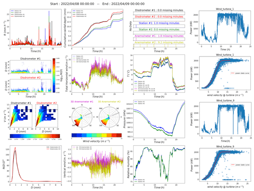
Figure 2 A quicklook of the RW-Turb data on 8 April 2022. The turbine power shown in the rightmost column is the property of Boralex; it is not available in the public database of RW-Turb (online quicklook). Descriptions of the plots can be found in the text.

Technical and working information on the turbines can be found in Vestas Wind Systems A/S (2023). Vestas V-90 was designed with a power configuration of 2.0 MW (rated power) and a pitch regulated with variable speed. The hub height of the turbines is 80 m: this is closer to the vertical height of the upper set of devices on the mast (location 1 at ≈78 m). The power state curves of the turbines can be seen in the last column of Fig. 2. They follow the cut-in, rated, and cut-out wind speeds (4, 12, and 25 m s⁻¹), with the majority of the points being around the rated power. Some clustering of power values can be seen at zero because of the treatment of negative power (power consumed for operation > power produced) as zeroes in data. The power output is sampled with time steps of 15 s.

2.3.2 Derived fields: available wind power and air density

Power production from turbines is analysed at the lowest available time step here of 15 s (4 Vestas V-90 with 2 MW managed by Boralex; see Fig. 1 for the location from the meteorological mast). The available power at the turbine for extraction can be approximated as

$$\begin{array}{}\text{(10)}& P_{\mathrm{a}}={\displaystyle \frac{\mathrm{1}}{\mathrm{2}}}\mathit{\rho }A{v}^{\mathrm{3}}{C}_{\mathrm{p}},\end{array}$$

where ρ is the air density at the wind turbine height (h_hub), A is the swept area of the turbine rotor, v is the wind velocity (m s⁻¹) approximated at the turbine height, and C_p is the power coefficient or Betz coefficient (for the Vestas-90 examined here, h_hub=80 m, A=6362 m², and the rated power is 2 MW). A strong limitation of this widely used formula is that it does not account for the wind spatial variability over the swept area. The value of the air density is often approximated as 1.255 kg m⁻³ (standard value at sea level 15 °C). However, it is known to show fluctuations and has been reported to have an effect on power generation at varying levels (Jung and Schindler, 2019; Ulazia et al., 2018). For the purpose of this analysis, air density was considered a varying quantity and estimated using the current official formula of the International Committee for Weights and Measures (CIPM), referred to as the CIPM-2007 equation that accounts for humidity (Picard et al., 2008):

$$\begin{array}{}\text{(11)}& \begin{array}{rl}\mathit{\rho }(T,P,H_{\mathrm{r}})& ={\displaystyle \frac{P{M}_{\mathrm{a}}}{Z(T,P,H_{\mathrm{r}})RT\left(K\right)}}\\ & \times \left\{\mathrm{1}-x_{\mathrm{v}}(T,P,H_{\mathrm{r}})\left[\mathrm{1}-{\displaystyle \frac{M_{\mathrm{v}}}{M_{\mathrm{a}}}}\right]\right\},\end{array}\end{array}$$

where T (°C), P (Pa), and H_r ($\mathrm{0}\le H_{\mathrm{r}}\le \mathrm{1}$) are the temperature, pressure, and humidity from the meteorological station at h_hub. The other derived parameters are as follows:

• T(K), air temperature (K; from T);

• Z, compressibility factor (a function of T and P);

• R, molar gas constant (J mol⁻¹ K⁻¹);

• x_v, mole fraction of water vapour;

• M_a, molar mass of dry air (g mol⁻¹); and

• M_v, molar mass of water (g mol⁻¹).

2.3.3 Sampling resolution, biases, and filtering of data

As can be seen in the turbine power state curves in Fig. 2 (last column), the vast majority of the turbine power (P_t) values are clustered around the rated value of 2.0 MW. However, when the available power (P_a) is calculated using Eq. (10), the values go far beyond the limitation of the rated power. This upper limit, along with the presence of zeroes, was found to bias the UM estimates of turbine power. This is addressed in Part 1 of this paper (Jose et al., 2024), and since it was possible to retrieve those biased values from the underlying field (P_a) by artificially imposing the biases, it was decided to use P_a as a field to study realistic correlation values. In the presented analysis, P_t is also included. However, this should be considered with the biases detected for which no corrections have been available so far.

Other than this bias from the rated power in the turbine, there were a few more concerns regarding the quality of the remaining data. On the basis of the data presented in Gires et al. (2022), UM analysis of the fields revealed that, even though the data are recorded at a finer resolution, the actual sampling resolution for studying variability may be coarser. Based on this insight, the fields are analysed here at lower resolutions than manufacturers claim (which still have high resolutions as far as the data are concerned). Table 1 summarizes the fields studied and their actual sampling resolution. This is applicable for instruments at locations 1 and 2 on the mast (Fig. 1).

Table 1 Details of the fields studied, their sources, and the actual sampling resolutions at which they were studied (based on results from Gires et al., 2022). The station parameters were taken at 15 s (instead of 16 s) to match the wind turbine power measurements.

Before proceeding to the analysis, the whole dataset was validated (November 2020 to May 2022) by checking for unusual entries and instrument downtime at both locations on the mast as well as the four turbines. Time steps were not considered for all of the fields if any one of the devices was not working. This included 5 months when the anemometer (17 June to 29 November 2021) and station (17 June to 11 November 2021) at location 1 on the mast were struck by lightning and had to be replaced, together with some time steps of turbine downtime (which were given as the interpolation in the unfiltered data) during March and June 2021. There were a few time steps where abnormal values were recorded for T, P, and relative humidity (RH); these were removed using a simple filter that replaced values of station parameters with “nan” (not a number) whenever the pressure was shown to be below 800 hPa. If nan was isolated, it was replaced by the average of the preceding and succeeding entries.

An event was considered strictly rain if there was a cumulative depth greater than 0.5 mm and separated by at least 15 min of a dry condition before and after. The converse of this criterion was employed to get dry events; events shorter than 5 min were discarded, together with events when any of the devices (including turbines) gave more than 30 % nan or 50 % zeroes. After data filtering, a total of 1488 rain events (and 2309 dry events) were obtained; events were identified from 2-year- and 3 month-long data (12 November 2020 to 9 February 2023). Further removal of events was performed in subsequent UM analyses to accommodate event sizes to the closest power of 2.

3 Multifractal analysis of the fields

One major interest of this campaign involving simultaneous measurement of wind and rain was the correlations between them across various scales. In this section, the validity of multifractal characterization of the fields is tested using the framework of UM; this is followed by a correlated multifractal analysis using the framework of JMF.

3.1 UM analysis of fields according to dry and rainy conditions

Before performing the joint analysis, the fields were individually studied for possible differences in behaviour under rainy and dry conditions using UM analysis. Rain and dry events were selected following the criteria mentioned in the previous section, and each of the fields in Table 1 was separately subjected to multifractal analysis for the selected events and ensembles (rain ensemble and dry ensemble). Of the events identified using the criteria mentioned before, the events with more than 30 % nan or zero were removed by checking the data across all the devices; this left 765 rain events (and 1203 dry events). To reduce the influence of the upper and lower thresholds on the turbine power, a further correction was employed where columns with more than 30 % nan or zero were removed equally across all the ensembles. For the UM analysis, sample sizes (N_sam) of 128 (32 min) fields at 15 s and 2048 (≈32 min) fields at 1 Hz were used. If an event was larger than the sample size (powers of 2 greater than N_sam), it was split into ensembles of length N_sam. For example, if the length of an event is 300 (75 min), it is trimmed to the nearest power of 2 (256, 64 min) so as to accommodate the time steps that give the largest rainfall cumulative depth; this was then made into an ensemble of size 128 (32 min) with two columns. To maximize the number of events in the analysis, events of length <N_sam but ≥80 % of N_sam (or powers of 2>N_sam) were included by extending their length to N_sam (or powers of 2>N_sam) from the dataset.

The results of an ensemble analysis of all the rain events are shown in Fig. 3 (fields at 15 s) and Fig. 4 (fields at 1 Hz). Wind velocity (v) was estimated as the horizontal resultant from u_x and u_y provided by the 3D sonic anemometer; P_a was derived from this using Eq. (10). Both quantities were initially estimated at an instrument resolution of 1 Hz (Fig. 3) and were also averaged to 15 s (Fig. 4). Since the air density (ρ) involves station parameters (at 15 s), the finest time step was limited by them to 15 s, which anyway corresponds to the available time step of the power production. For illustration purposes, only Turbine 1 (the turbine closest to the mast; Fig. 1) is shown. The other turbines give similar estimates. The rest of the fields were taken from instruments at location 1 of the mast (≈80 m height), which is on a similar horizontal plane to the turbine hubs.

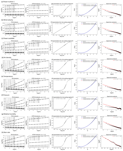
Figure 3 UM plots of rain events from 11 December 2020 to 3 June 2021 (6 months) for all the fields studied at the lowest instrumental resolution of 15 s (except for the rain rate at 30 s). For the ensemble of 756 events at a sample size of 128 (32 min), fluctuations of the field were used for the station fields and the rest for the direct field. The spectral plots here are from direct data.

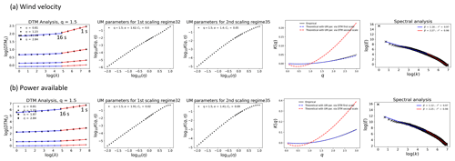
Figure 4 UM plots of rain events from 12 November 2020 to 9 February 2023 (∼ 2 years and 3 months) for the (a) wind velocity and (b) power available studied at the lowest instrumental resolution of 1 Hz. The ensemble of 213 events had a sample size of 2048 (≈ 32 min). α was estimated from the slope of the DTM curve at η=0. The FIF of the field was used. The spectral plots here are from direct data.

The UM plots for each field as an ensemble of all the rain events are given in Figs. 3 and 4 for the time period considered (the corresponding plots of the dry events are given in Appendix Figs. A1 and A2). The value of the non-conservative parameter H was too high for direct UM analysis of the station fields T, P, RH, and ρ (H∼0.9 and β∼2.8). This was reduced along with the spectral slope to conservative values by considering the fluctuations of the fields, which is a common approximation for fractional differentiation (H∼0 and β<1). They all gave similar C₁ values (∼ 0.06). ρ and RH gave similar α values (∼ 1.7) as well, while P and T gave values of 1.39 and 1.2. For the P_a and v 1 Hz data, two scaling regimes were observed with a break closer to 15 s (16 s in actuality; Fig. 4). Direct data gave estimates of H that were acceptable (H<0.5) for performing UM analysis when 15 s was used as the finest time step (Fig. 3: H∼0.2 and β∼1.4), while the smaller scale (1 Hz to 15 s) gave very non-conservative values (H∼0.6 and β∼2.2). For P_a and v at 1 Hz (1 Hz to 15 s), taking the fluctuations reduced H too much (∼ −0.2 and −0.4 respectively). In examining these smaller-scale variations, fractionally integrated flux (FIF) is recommended for retrieving the conservative part: this gave H∼0 (Fitton, 2013; Gago et al., 2022). For P_a and v, the larger-scale (from 16 s to 32 min) values of α and C₁ were 1.91 and 0.021 (α) and 1.62 and 0.0093 (C₁); for finer scales (1 Hz to 16 s), α values were smaller and C₁ values larger: 1.40 and 0.09 (α) and 1.38 and 0.05 (C₁). The possibility of two scaling regimes for 15 s fields is not considered here (Fig. 4), as it was convenient to compare rain and dry conditions in a single regime for consistency.

Figure 5 Comparison between UM parameters of the rain- and dry-event ensemble: (a) α, (b) C₁, and (c) H.

From the ensemble analysis, slightly increased values of α were observed for the rain ensemble in comparison to the dry ensemble (plots shown in Fig. 5) for all the fields. Since C₁ is rather similar, it can be inferred that the fields exhibit more variability when rain is present (Fig. 5a and b). With this insight, rain events are analysed in detail individually.

3.2 Joint analysis of fields according to rain

The scaling and multifractal properties of the fields were examined for rain (and dry) events individually and as an ensemble previously. The influences of some of these fields are obvious by virtue of definition: available wind (and hence the power extracted from the turbines P_t) and air density (ρ) are derived from wind velocity (v) and station fields (T, P, and RH). To understand the influence of rain on wind power, it is essential to understand its natural correlation with wind (and hence P_a). Using the previously defined JMF, it is possible to analyse two conservative fields together and to estimate the correlation exponent between them when one is expressed as a multiplicative combination of the other with an independent multifractal field. For example, the correlation of P_a with v can be explored by expressing them as ${P_{\mathrm{a}}}_{\mathit{\lambda }}=\frac{{v_{\mathit{\lambda }}}^a{Y_{\mathit{\lambda }}}^b}{\langle {v_{\mathit{\lambda }}}^a{Y_{\mathit{\lambda }}}^b\rangle }$, where λ is the resolution of the field, Y_λ is another UM field, and a and b are the correlation exponents between them (see Sect. 2.2).

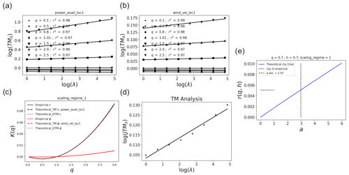
Figure 6 (a) TM plots of P_a, (b) TM plots of v (log–log plots of Eq. 3), (c) K(q) plots for both fields, (d) TM plots for the joint field, and (e) estimation of the JMF parameter a for an ensemble of all moderate rain events at location 1. Rain events were analysed as an ensemble of size 128 from 12 November 2020 to 9 February 2023 (∼ 2 years 3 months).

With this framework, the correlations of P_t, P_a, v, and ρ with each other (and with the station fields) are explored here according to the rain rates. For this purpose, the rain events (12 November 2020 to 9 February 2023) were classified into six groups based on the rain rate (with a 5 min moving average so that events are characterized by their intense portions). For this, the criteria in Tokay and Short (1996) were used (only rain rates), rain events were selected, and separate ensembles (N_sam of 128 time steps or 32 min) were created for each of the six rain groups. Since JMF involves expressing fields as combinations of each other, the finest resolutions of the fields were limited by the highest actual sampling resolution (15 s, Table 1). JMF plots of P_a and v for an ensemble of all moderate rain events at location 1 are shown in Fig. 6 as an illustration for pedagogical purposes. Values of a closer to 3 (as expected from Eq. 10) and good scaling were obtained with an $r_{\mathrm{JMF}}^{\mathrm{2}}$ value of 0.98. The variations of JMF parameters a and IC are given in Fig. 7 for location 1; similar estimates were obtained for location 2 as well. Overall, very small increases in the values of IC and a were observed with an increase in the rain rate (5 min moving average) when correlations of P_a with v and the station fields were considered (Fig. 7b). A similar trend was observed when v was analysed against P_a and the station fields (Fig. 7c) and also when ρ was analysed against the rest of the station fields (Fig. 7d). The quality of scaling $r_{\mathrm{JMF}}^{\mathrm{2}}$ did not show any trend like the values of a or IC. The effect of the previously mentioned thresholds on turbine power (due to rated power and negative power) seems to have a stronger bias in JMF; the JMF of P_t with every field across various rain types gave estimates far lower than that of P_a, with comparatively worse scaling. The estimates were found to be even lower when the 30 % correction was not employed (values of a close to 0); without the correction, P_t also gave inconsistent values of $r_{\mathrm{JMF}}^{\mathrm{2}}$, with values going lower than 0.1 in some cases. This behaviour was consistent across all four turbines. For P_t (Fig. 7a), this poor scaling is not surprising considering the biases established earlier. As a result, the interpretation of trends is not advisable, and it is better not to consider values of JMF parameters from P_t as they are not robust enough.

Here, values were estimated from the joint scaling function r(q,h) at the same moment order ($q=h=\mathrm{0.7}$) for both fields based on sensitivity analysis around various $q/h$ options (for both individual and ensemble analyses). We checked that the values of q_s and q_D (moments corresponding to the sampling limitation and divergence respectively) were above h+q, h, and q for all of the cases analysed here, as desired. This is required to obtain reliable values in JMF (Gires et al., 2020a).

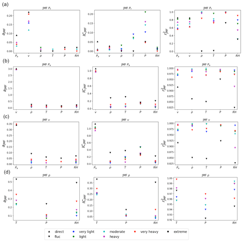
Figure 7 Variation of JMF parameters a, IC, and quality of scaling $r_{\mathrm{JMF}}^{\mathrm{2}}$ between (a) P_t (Turbine 1), (b) P_a, (c) v, and (d) ρ as well as other fields according to the type of rain (on the basis of a 5 min moving average of the rain rate with criteria in Tokay and Short, 1996). The rain events of each class were analysed as an ensemble of size 128 from 12 November 2020 to 9 February 2023 (∼ 2 years and 3 months).

From early UM analysis, it was decided that, for fields at 15 s resolution, all station fields need to be analysed as fluctuations, while wind (v) and wind-derived fields (P_a and P_t) can be studied directly. Though the desired conservative field is retrieved using this choice, it could cause issues in JMF as this could be a combination of a direct field and an indirect field (fluctuations or FIF). For example, in Fig. 7a, P_a is a direct field, while the fields with which its correlations are analysed (ρ, T, P, and RH) are fluctuations. In UM this is discussed in the previously defined Eq. (5). To recap, a non-conservative field ψ_λ (i.e. $\langle {{\mathit{\psi }}_{\mathit{\lambda }}}^{\prime }\rangle \ne$ 1) in UM can be expressed in terms of the underlying conservative field (ε_λ retrieved through fluctuations or FIF 〈ε_λ〉 = 1) as ${\mathit{\psi }}_{\mathit{\lambda }}{=}^{\mathrm{d}}{\mathit{\epsilon }}_{\mathit{\lambda }}{\mathit{\lambda }}^{-H_{\mathit{\epsilon }}}$. Here H_ε is the non-conservative parameter that characterizes the variation of the mean ε_λ across resolutions λ. When two fields ${{\mathit{\epsilon }}_{\mathit{\lambda }}}^{\prime }$ and ${{\mathit{\varphi }}_{\mathit{\lambda }}}^{\prime }$ (^′ suggests their non-conservative nature) are analysed as a multiplicative combination in JMF, only their respective conservative parts can be used (${\mathit{\epsilon }}_{\mathit{\lambda }}=\frac{{{\mathit{\varphi }}_{\mathit{\lambda }}}^a{Y_{\mathit{\lambda }}}^b}{\langle {{\mathit{\varphi }}_{\mathit{\lambda }}}^a{Y_{\mathit{\lambda }}}^b\rangle }$). Hence, the estimated JMF parameter a does not correspond to the full field. If one field is direct and the other is a retrieved conservative part (fluctuation or FIF), the values of a could be biased as the underlying H values (H_ε and H_ϕ) are not considered in its estimation.

To assess the possible influences of this, a sensitivity analysis was performed using two known fields: P_a (ε_λ) and the field it was derived from (ϕ_λ): P_a∝v³ (Eq. 10). The previously used dataset – respective ensembles of rain events from 12 December 2020 to 3 June 2021 (6 months with N_sam 128) – was used for this purpose; the results are displayed in Table 2 while using P_a and v as direct fields, a in the JMF analysis, the exponent value in Eq. (10) (Table 2) with good joint scaling ($r_{\mathrm{JMF}}^{\mathrm{2}}$), and IC. Though H is not non-zero for either of the fields, them being similar gave a difference close to zero (H_ε−H_ϕ). Similarly, a closer value of a (a=2.75) was obtained when both fields were taken as the FIF. From the samples in Fig. 8a and b, it can be seen that the fields follow the same pattern when both are direct or FIF (Fig. 8b follows the same pattern as the direct field in Fig. 8a, while the fluctuations in Fig. 8c do not), with the difference in amplitude from the mean line following the proportionality exponent in Eq. (10). When both fields were taken as fluctuations, values of a closer to 1 were obtained. This is rather consistent as fluctuations take the difference between the time steps and are expected to show a proportional relationship as the fields are already related. However, this also places the analysis at an apparent disadvantage, as using JMF on fluctuations only retains the proportionality but not its order. This can be observed in the sample in Fig. 8c, where both fields appear similar (following P∝v rather than the original P∝v³). In the remaining cases, when neither field had similar values of H, the estimates of a were decreased, except when H_ε was significantly less than H_ϕ (FIF – P_a – and direct – v). This might have to do with ε_λ (P_a) being the field estimated based on ϕ_λ or v ($P_{\mathrm{a}}=\frac{v^a{Y_{\mathit{\lambda }}}^b}{\langle v^a{Y_{\mathit{\lambda }}}^b\rangle }$), while the JMF analysis tries to express it in terms of fluctuations of ϕ_λ, which does not follow the same time step pattern as the direct data or FIF (Fig. 8c).

Table 2 Sensitivity analysis using available power P_a (ε_λ) and wind velocity v (ϕ_λ), where JMF parameters are estimated for different combinations of data – direct (dir), fluctuations (fluc), and FIF (fractionally integrated flux). Data from 12 December 2020 to 3 June 2021 at the 15 s fields were re-normalized for comparison. Time series of fields corresponding to the bold values are shown in Fig. 8.

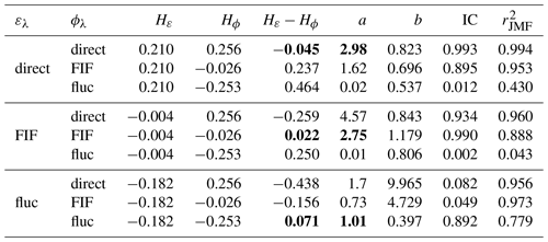
Figure 8 (a) Direct data of the P_a and v. (b) FIF of the P_a and v. (c) Fluctuations of P_a and v for one sample (N_sam=128) of the data analysed (from 12 December 2020 to 3 June 2021 at 15 s, fields re-normalized for comparison). Between the plots, it can be seen that the direct data and FIF follow a similar data pattern, while the fluctuations do not.

Though the biases from the analysis of JMF are acknowledged here, there is no correction available at this point, and this should be investigated further in the future. Of the results presented in Fig. 7, all the JMF analyses except for P_a–v combinations are affected by this. More research is needed to account for this when accurate retrieval of correlation parameters is of interest. Even with biases, the values of a and IC are still strong indicators for comparing two multifractal fields under various atmospheric conditions as illustrated in Fig. 8.

4 Effect of rain type and wind direction on power production

4.1 Possible influence from convective and stratiform rain

The yearly average cumulative depth of rain on the wind farm was found to be ∼ 600 mm and, of the 6 months of rain events (213) studied, only 20 could be classified as heavier rainfall events (heavy, very heavy, and extreme). Because of this, it was speculated that the lack of a very strong correlation between the rain and the power produced could be due to the rainfall events not being strong enough (apart from the known bias from the threshold due to the rated power). To test this hypothesis, efforts were made to identify the rain events as convective or stratiform. While convective rains have highly concentrated intensities, stratiform rains are more horizontally spread with lower intensities (Houze, 2014; Marzano et al., 2010). Several criteria have been used to detect this indirectly in the literature; simple ones are the classification on the basis of the rain rate exceeding a particular value. Popular criteria using the rain rate are in Bringi et al. (2003), where convective rain samples are considered to be those with the rain rate, R, ≥5 mm h⁻¹, and the standard deviation (SD) over five consecutive 2 min samples >1.5 mm h⁻¹ (referred to as BR03 from here on). Tokay and Short (1996) proposed an empirical classification based on DSD parameters by identifying the shift from spectra dominated by small to medium drops (stratiform) to spectra dominated by large drops (convective) for similar rain rates (referred to as TS96 from here on). Attributing a temporal shift in the DSD parameters (shape parameter Λ) to shifts in the rainfall size distribution, they suggested a value of $\mathrm{\Lambda }=\mathrm{17}{R}^{-\mathrm{0.37}}$, above which precipitation can be considered convective (stratiform if below).

To explore this, DSD parameters of rain events on the wind farm were estimated assuming a gamma distribution (following the method of moments used in Jose et al., 2022). From 12 November 2020 to 9 February 2023, from the filtered list of events, a total of 150 was identified as convective (using the TS96 criteria). However, only 37 events were above 32 min and hence among the events subjected to UM and JMF analysis before; 25 events of comparable length were selected from both convective and stratiform sides, where at least 70 % of the time steps followed the TS96 criteria. Two turbines were examined for these events – Turbines 1 and 9 (closest to and farthest from the mast): a possible difference in turbine power between the convective and stratiform events is not obvious from the mean, standard deviation, or state curves (Fig. 9). This obviously comes with the disclaimer that it was a simple test using limited events without considering other complexities. For example, the dispersion being greater at Turbine 9 (as this is farthest from the mast from where the velocity was measured) is ignored. However, considering the predominant stratiform nature of rain at the location studied, the hypothesis of needing stronger rainfall to see the proper correlation between the power produced and rainfall is still worth exploring in the future.

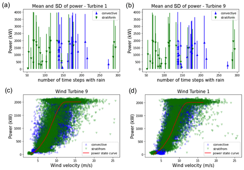
Figure 9 Mean and standard deviation of the power produced, P_t, for (a) Turbine 1 (closest to the mast) and (b) Turbine 8 (farthest from the mast). The power state curve is from selected convective and stratiform events for (c) Turbine 1 (closest to the mast) and (d) Turbine 8 (farthest from the mast).

4.2 Possible influence from the wind direction

The turbines are aligned south-east within a 4 km radius; to the south of the mast a small groove is located at roughly 160 m, and a larger one is located in the east at around 100 m (Fig. 1). To see the effect of these topographical features and the spread of vegetation around the mast, wind directions were identified as shown in Fig. 10, with the mast as the centre. Based on this, the average wind direction was calculated for rain events using u_x and u_y from the 3D anemometer at location 1. Based on the position of immediate vegetation around the mast, the wind was grouped into three zones – least influenced (69), most influenced (60), and turbine direction (7 events). As this was done manually, on the basis of the vicinity and size of the vegetation, not all directions are considered in this classification (specified in Fig. 10).

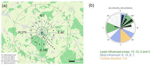
Figure 10 (a) Location of the wind farm and the identified wind directions. (b) Number of events corresponding to the direction (the colours show the direction classes, the lengths of the black arcs correspond to the number of events, and the thickness corresponds to the average magnitude) and the three groups considered.

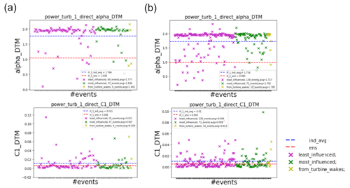
Figure 11 Variation of α and C₁ according to wind direction for (a) rain events and (b) dry events. The values of the ensemble and the average value of the individual events are shown using red and blue lines.

The variations of the UM parameters of turbine power closest to the mast (Turbine 1) according to the wind classes are shown in Fig. 11 for rain and dry events. No obvious difference was observed: similar results were observed for the rest of the turbines as well. Due to the previously identified bias from rated power in the UM analysis, it is not possible to say exactly whether this is exact behaviour or not. This was not explored further in this thesis. Factors known to affect power production at the turbine wake, such as mixing of moist air Obligado et al. (2021) or dynamic effects from inertial particles (Smith et al., 2021), were not considered here either.

4.3 Power state curve under different rain and wind conditions

All the studies so far were event-focused, as this provides the behaviour of a continuous field for a given period of time. In this section, instantaneous (subject to the recording time step) empirical turbine power (P_t) was examined according to the type of rain (same criteria as those of the events) and wind (14 classes at intervals of 2 m s⁻¹). For this, all the individual time steps from 12 November 2020 to 9 February 2023 were grouped according to R and v at that instant at a time step interval of 1 m. A total of 503 085 1 min long time steps were grouped in this way. Figure 12a shows the power curves for each rain class of Turbine 1 alongside the theoretical state curve provided by the manufacturer (dotted red line). Singular values of power were obtained by averaging the empirical power registered at all the time steps corresponding to that particular wind class. This is then visually compared with the state curve of dry (no-rain) time steps (solid yellow line) (Fig. 12a and c) and the percentage change (${\mathrm{Power}}_{\mathrm{rain}}-{\mathrm{Power}}_{\text{no-rain}})/{\mathrm{Power}}_{\text{no-rain}}$ (Fig. 12b).

In lower wind velocity classes (below 10 m s⁻¹), the average power of all the rain classes is above that of the theoretical state curve (except for “extreme”, which only trails the power curve till 8 m s⁻¹). Lower rain class time steps generate more power in this region than heavier ones, together with the dry time steps; this is progressively reduced as we move towards the rated wind speed (from a 60 % difference to almost 0 % near 12 m s⁻¹) and above. Around the rated power, the state curves of all the rain classes go below the state curve of the manufacturer, with the difference regained as the curve moves towards the cut-off speed (25 m s⁻¹). When compared with that of the dry state curve, it can be seen that very light, light, and moderate rain follows more closely, while the rest trails below (more clearly observed in terms of the percentage in Fig. 12b). It can be inferred that there is a general increase in the power produced under low rain and wind conditions. However, this behaviour is observed below the rated velocity of the turbine. For stronger winds (above the rated wind velocity), the power produced during lower rains remains the same, while heavier rains provide much reduced values. It can be roughly said that, the heavier the rainfall, the sooner the fall of power below that expected from the state curve provided by the manufacturer.

However, this observation does not involve the same number of 1 min time steps for all the rain classes. For example, the “no-rain” time steps are far larger in number than the rain events (Fig. 12d): in the case of the rain events, the higher the value of the rain rate, the lower the number of time steps available (Fig. 12d and e). To improve the statistics, the events in and above heavy were combined into one class; the shift observed before can be seen in this case as well (Fig. 12c). This disproportionate number of points is also the reason for the sudden dips in the state curves for the higher rain classes.

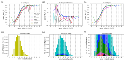
Figure 12 Power state curves from averaging the power values of Turbine 1 at a time step of 1 min: (a) state curves for all the rain classes, (b) percentage change from the state curve corresponding to time steps with no rain, and (c) state curves for rain classes (rain steps in and above “heavy” are considered to be one – heavy). The second column shows histograms of the time steps of different rain classes: (d) no rain, (e) all rain classes, and (f) all rain classes zoomed in for more rain.

Figure 13a shows the same information but at a time step of 10 min. To respect the scale change, rain rates were grouped as per singularities (γ); rainfall singularities (γ_r) for the rates at 1 min were used to categorize rain rates at 10 min (${\mathit{\gamma }}_{\mathrm{r}}=\frac{\log \left(\mathrm{rain}\mathrm{rate}\right)}{\log \left(\mathit{\lambda }\right)}$). This reduces the average rain rates to the corresponding lower values.

However, this also truncates the extreme rain time steps (of 10 min) due to the lack of points; this can be seen in Fig. 13e and f and is reflected in the uneven distribution of the state curves for the higher rain steps. Still, as seen before (Fig. 12a), rain below heavy shifts from the theoretical state curve around the 10–12 m s⁻¹ velocity class here as well. This can be seen in a cleaner way in Fig. 12b, where higher rain time steps are combined into one – heavy. Figure 12b shows the percentage difference of this shift with respect to values for no rain.

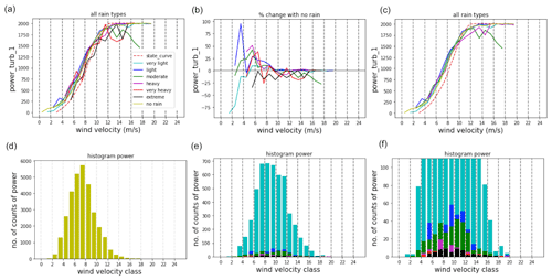
Figure 13 Power state curves by averaging the power values of Turbine 1 at a time step of 10 min: (a) state curves for all the rain classes, (b) percentage change from the state curve corresponding to time steps with no rain, and (c) state curves for rain classes (rain steps in and above “heavy” are considered to be one – heavy). The second column shows histograms of the time steps of different rain classes: (d) “no rain”, (e) all rain classes, and (f) all rain classes zoomed in for higher rain.

To summarize this observation in terms of turbine state curve values, rain steps below heavy fall below the theoretical state curve after 10–12 m s⁻¹, which corresponds to the transition of the power curve to the rated power (12 m s⁻¹). It can be roughly inferred that, the higher the rain rate, the lower the velocity at which the power falls below the expected value for the velocity at that time step. Also, after the cut-in velocity (4 m s⁻¹), heavier rains show a higher percentage difference from those with no rain (Figs. 12b and 13b).

As different shifts from the theoretical state curve were observed for different rain classes, the JMF analysis was re-performed earlier by dividing the events on the basis of wind velocity. Since the shift happened around the rated speed of 12 m s⁻¹, the events were grouped into “<10” and “>10”: 10 m s⁻¹ was selected on the basis of the above-mentioned observations as well as the consideration of some leeway for the shift to rated power. The variation of the JMF parameter a is shown in Fig. 14. The trend observed in Fig. 7 is mostly lost here since splitting the events on the basis of velocity reduced the number of datasets available for analysis, especially for higher rain events. Further, the biases associated with the empirical power (P_t) make meaningful interpretation difficult. It is not possible to characterize the behaviour observed from time-step-based analysis of events with the current data and methodology. Furthermore, since the velocity is averaged over larger time periods when it comes to events, the information is diluted to some extent as well.

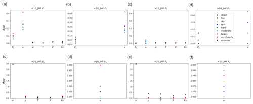
Figure 14 Variation of the JMF parameter a for an ensemble of events (dry and various rain classes) at a sample length of 32 min. The first row shows events with average wind velocity <10 m s⁻¹ (a) P_t (Turbine 1), (b) P_a, (c) v, and (d) ρ and other fields according to the type of rain (on the basis of a 5 min moving average of the rain rate with criteria in Tokay and Short, 1996). The rain events of each class were analysed as an ensemble of size 128 from 12 November 2020 to 9 February 2023 (∼ 2 years and 3 months).

5 Conclusion

From Gires et al. (2022), it was seen that the actual sampling resolutions relevant for studying the variability of meteorological fields measured with the help of a mini station (T, P, RH, and $\mathit{\rho }=f(T,P,\mathrm{RH})$) and that for 3D anemometer fields (v and P_a) were 15 and 1 s respectively (instead of 1 and 0.01 s). Using the data averaged to these reliable frequencies, UM behaviour, together with the JMF correlation between P_t, P_a, v, ρ, T, and RH, was analysed to gain insights into the correlation with rainfall, which is poorly understood. However, direct analysis of turbine power was found to be difficult since the output from wind turbines is limited by a maximum or rated power; in time series analysis this acts as an upper threshold, resulting in reduced estimates of UM parameters. This bias is identified in the theoretical framework of UM and is also illustrated using discrete cascades of numerical simulations of conservative multifractal fields in Part 1 of this joint paper. Due to the presence of these biases in P_t, the actual wind power available at the turbine hub for extraction ($P_{\mathrm{a}}=f(v,\mathit{\rho })$) was primarily used instead as the main field for joint analysis.

For UM analysis, fluctuations of the fields were required for the station fields to retrieve conservative fields so that estimates of TM and DTM were not biased. For the anemometer fields, direct field analysis was acceptable in large-scale regimes (from 15 s), while small scales (0.01 to 15 s) required retrieval of conservative fields through FIF. From UM analysis of rain and dry events as ensembles, it was found that almost all the fields showed a slight increase in variability with rain (larger α and similar C₁) in the scale range from 15 s to 32 min, over which a unique scaling behaviour is identified. An opposite trend was observed for finer scales of P_a and v (0.01 to 15 s). Joint analysis of P_a, v, and ρ with each other and with the station meteorological fields (all fields at 15 s) revealed an increasing trend in the value of the JMF correlation exponent a and IC with the rain rate. However, this is not without biases, since the station fields fluctuated, while the anemometer fields were directly in the analysed scaling regime. The influence of this bias is identified and commented on. Also, detailed sensitivity analyses were performed to identify the possible effects of wind direction and rainfall type on the power production in turbines. No clear trends in the results were identified. Grouping of instantaneous time steps of power according to velocity and rain revealed an interesting departure from the state curves for different rain classes. With lower velocities (below the rated power) and lighter rains, the turbines provided more power than expected from their theoretical state curve. At higher velocities, lighter rain time steps more or less provided expected values of empirical power, while those of heavier rains provided much less. However, it was not possible to identify this in an event-based analysis in the current study (Fig. 14).

Future methodological developments in the JMF framework are proposed here to handle the biases when analysing the direct and indirect fields. Though the effect of the upper threshold is identified in the framework, further work is required to precisely quantify the bias. Also, considering the predominant stratiform nature of rain at the measurement location, studying the correlations under convective conditions is encouraged, for the future, to expand the understanding of correlations between rainfall and wind power production. The trend observed with the power state curve needs more careful future examination as well. The results here are from instantaneous data analysis: this needs to be complemented with simulations and a better understanding of the physical process leading to this. Though the changes in atmospheric conditions are considered here to some extent, the effects due to the physical nature of the blade (weight, roughness) and its aerodynamic interaction in flow are missing.

Appendix A: UM plots of dry events as an ensemble for all the fields

The UM plots of dry events at the RW-Turb mast, location 1, are all at a resolution of 15 s.

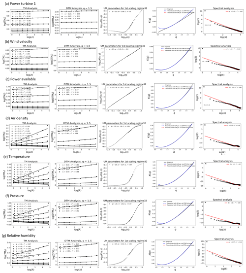
Figure A1 UM plots of rain events from 11 December 2020 to 3 June 2021 (6 months) for all fields studied at the lowest instrumental resolution of 15 s (except for the rain rate at 30 s). An ensemble of 213 events at a sample size of 128 (32 min) and fluctuations of the field were used for the station fields, while direct field was used for the rest. The spectral plots here are from the direct data.

Figure A2 UM plots of dry events from 11 December 2020 to 3 June 2021 (6 months) for (a) wind velocity and (b) power available studied at the lowest instrumental resolution of 1 Hz. The ensemble of 213 events at a sample size of 2048 (≈32 min) α was estimated from the slope of the DTM curve at η=0. The FIF of the field was used; the spectral plots here are from the direct data.