the Creative Commons Attribution 4.0 License.
the Creative Commons Attribution 4.0 License.
 | 19 Sep 2024
Characterisation of Dansgaard–Oeschger events in palaeoclimate time series using the matrix profile method
Susana Barbosa
Maria Eduarda Silva
Denis-Didier Rousseau
Palaeoclimate time series, reflecting the state of Earth's climate in the distant past, occasionally display very large and rapid shifts showing abrupt climate variability. The identification and characterisation of these abrupt transitions in palaeoclimate records is of particular interest as this allows for understanding of millennial climate variability and the identification of potential tipping points in the context of current climate change. Methods that are able to characterise these events in an objective and automatic way, in a single time series, or across two proxy records are therefore of particular interest. In our study the matrix profile approach is used to describe Dansgaard–Oeschger (DO) events, abrupt warmings detected in the Greenland ice core, and Northern Hemisphere marine and continental records. The results indicate that canonical events DO-19 and DO-20, occurring at around 72 and 76 ka, are the most similar events over the past 110 000 years. These transitions are characterised by matching transitions corresponding to events DO-1, DO-8, and DO-12. They are abrupt, resulting in a rapid shift to warmer conditions, followed by a gradual return to cold conditions. The joint analysis of the δ18O and Ca2+ time series indicates that the transition corresponding to the DO-19 event is the most similar event across the two time series.
- Article
(2561 KB) - Full-text XML
- BibTeX
- EndNote


Palaeoclimate time series reflect Earth's climate in the distant past based mainly on proxies derived from records such as sediments, ice cores, or speleothems. One of the most extensively studied palaeoclimate time series is that of oxygen isotope ratios (δ18O) retrieved from Greenland ice cores in the context of the North Greenland Ice Core Project (NGRIP) (Andersen et al., 2004; Rasmussen et al., 2014). The concentration of δ18O, as measured in the ice, serves as an indirect proxy of the air temperature at the ice core location.
The ice cores retrieved from the Greenland ice sheet revealed the occurrence of rapid warming events, which occurred over a few decades. Such abrupt transitions are designated Dansgaard–Oeschger (DO) events, during which climate conditions alternated between fully glacial (so-called stadial) and relatively mild (interstadial) conditions (Dansgaard et al., 1982; Johnsen et al., 1992; Rasmussen et al., 2014). These abrupt transitions, on average, are approximately 12 °C, with a range of 5 to 16 °C (Kindler et al., 2014). They exhibit a distinctive sawtooth shape, with rapid, decadal, increases in δ18O from Greenland stadial (GS) to Greenland interstadial (GI) conditions, followed by slow relaxations back to GS conditions on timescales of centuries or millennia. However, it should be noted that not all DO events have the same shape or duration (Rousseau et al., 2017; Lohmann, 2019).
DO events are particularly observable in the Greenland ice core records, but similar transitions were identified in diverse palaeoclimate records (e.g. Rousseau et al., 2017; Corrick et al., 2020; Bagniewski et al., 2023; Held et al., 2024), and thus DO events have been used for “wiggle matching” of records with no accurate dating information (e.g. Peterson et al., 2000; Lauterbach et al., 2011). The objective identification of DO events, other than by visual inspection, is then of critical importance.
The original identification of DO events was conducted by visual inspection of the NGRIP δ18O time series. These “canonical DOs” (Rousseau et al., 2022) and further transitions were also identified visually by Rasmussen et al. (2014), who resorted to not only the δ18O record, but also the concurrent Ca2+ proxy record. An algorithm was developed by Lohmann and Ditlevsen (2019) for the characterisation of DO events based on their sawtooth shape. However, the approach does not identify the events themselves. Rather, it relies on the previous visual identification by Rasmussen et al. (2014). A method based on the Kolmogorov–Smirnov (KS) test was developed by Bagniewski et al. (2021), which allows the identification of the canonical DO events in addition to other transitions that were previously unidentified by visual inspection. Although the method allows for the detection of individual jumps in the records towards either cold–warm or dry–wet conditions, it does not provide any information on their magnitude. Recurrence plots (e.g. Marwan et al., 2007) and measures of recurrence quantification analysis such as the recurrence rate (Marwan et al., 2013) allow on the other hand for the identification of the dominant changes in a record's characteristic timescale (Bagniewski et al., 2021; Rousseau et al., 2023a, b).
Given that DO events can be considered a recurring pattern in a palaeoclimate time series, algorithmic methods for the extraction of similar patterns from a time series can be applied to characterise these particular patterns. In this study the matrix profile approach (Yeh et al., 2016) is employed to describe DO patterns in the Greenland ice core records. The methodology and data are described in Sects. 2 and 3, respectively. The results of the matrix profile approach applied to palaeoclimate time series are presented in Sect. 4. Methodological and interpretative constraints are discussed in Sect. 5, and concluding remarks are given in Sect. 6.
The matrix profile approach is described in detail in Yeh et al. (2016, 2018) and the references therein. This overview provides only a brief summary of the methodology. Readers are referred to the original references for further details.
For a real-value time series of length n, a sub-sequence Ti,m of length m is a continuous subset of the values of T: . The matrix profile is an ordered vector of the Euclidean distances between the most similar (shortest distance) sub-sequences, considering all possible sub-sequences of T obtained by sliding a window of length m across T. The distance is measured using the Euclidean distance between z-normalised sub-sequences with a mean of 0 and a standard deviation of 1 (Agrawal et al., 1993). The matrix profile is defined as the distance between a sub-sequence and its most similar sub-sequence, regardless of its location. That location is stored in the profile index. The profile index is a companion vector that stores the position of the nearest neighbour of each sub-sequence. The matrix profile and the matrix profile index are two data structures that annotate a time series with the distance and location, respectively, of the nearest neighbours of all its sub-sequences (in itself or in another time series).
The brute-force obvious algorithm to compute the matrix profile requires the computation of a large number of Euclidean distances equal to . While this complexity 𝒪((n−m)2) is not a problem in the case of the typical short lengths of palaeoclimate time series, it can easily become prohibitive for even modestly sized time series. Scalable and fast algorithms have been developed to tackle this issue, reducing the complexity of matrix profile calculations to 𝒪(n) (Yeh et al., 2018). The scalability and computational efficiency of the matrix profile are not what makes it an attractive tool in itself, but the variety of useful analytical tasks that can be performed based on the matrix profile is (Zhu et al., 2020).
The matrix profile enables the identification of motifs in the time series, corresponding to sub-sequences that are highly similar to each other. The (tying) lowest points in the matrix profile correspond to the locations of the optimal time series motif pair, i.e. the pair of sub-sequences that are most similar (Mueen et al., 2009): and dist dist, with , and dist the z-normalised Euclidean distance between the sub-sequences. The parameter w imposes a constraint on the relative positions of the sub-sequences in the motif, ensuring a gap between the sub-sequences of at least w values. This exclusion zone is intended to exclude trivial motifs as described in Lin et al. (2002). The exclusion zone thus defined enables the avoidance of trivial matches of a sub-sequence with itself or of largely overlapping sub-sequences. For a top motif of the most similar sub-sequences, which are separated by D1,min, neighbouring similar sub-sequences can be obtained by considering the sub-sequences within distances, where R is a small integer value (typically ≤2). The definition of a first-order motif can be generalised to that of a kth-order subsequent motif (where k is an integer number) by considering the following nearest pair of sub-sequences after excluding all sub-sequences belonging to prior motifs.
For a single time series T, the matrix profile stores the Euclidean distance from a sub-sequence Ti,m to its most similar sub-sequence. The concept can be extended to two time series TA and TB (which may have different lengths), with the join matrix profile containing the Euclidean distances between all sub-sequences in TA and their most similar sub-sequence in TB. The join motifs reflect the most similar patterns between the two time series (Yeh et al., 2017, 2018).
The Python code stumpy (Law, 2019) is employed to perform the matrix profile analysis. The R statistical software (version 4.1.3, R Core Team, 2022) is employed for the visualisation of the matrix profile results.
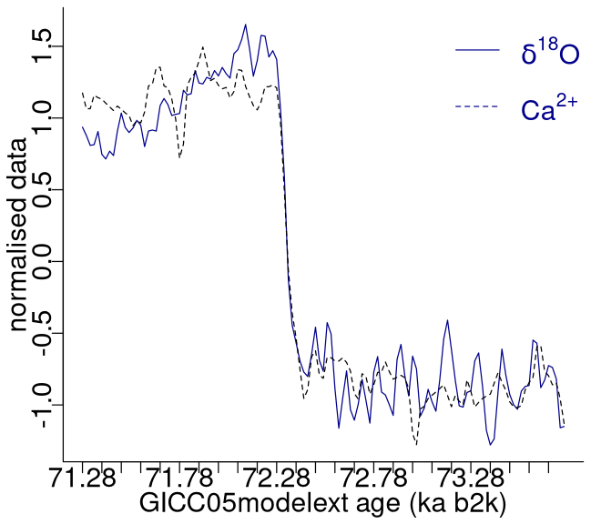
The analysis presented here applies to the 20-year-resolution time series of δ18O and calcium ion (Ca2+) concentrations from the NGRIP ice core on the GICC05modelext timescale (Rasmussen et al., 2014; Seierstad et al., 2014). The time series encompasses the interval from 107.6 to 10.2 ka b2k (before AD 2000), with 4869 data points in total. While the oxygen isotope ratio is a proxy for air temperature, calcium is a proxy of atmospheric dust (Fuhrer et al., 1999), reflecting changes in dust sources and transport pathways (Fischer et al., 2007). The time series are presented in Fig. 1, with the Ca2+ record represented on a reverse logarithmic scale, in line with the approach outlined by Rasmussen et al. (2014). A small number of missing values in the Ca2+ time series, <1%, were linearly interpolated.
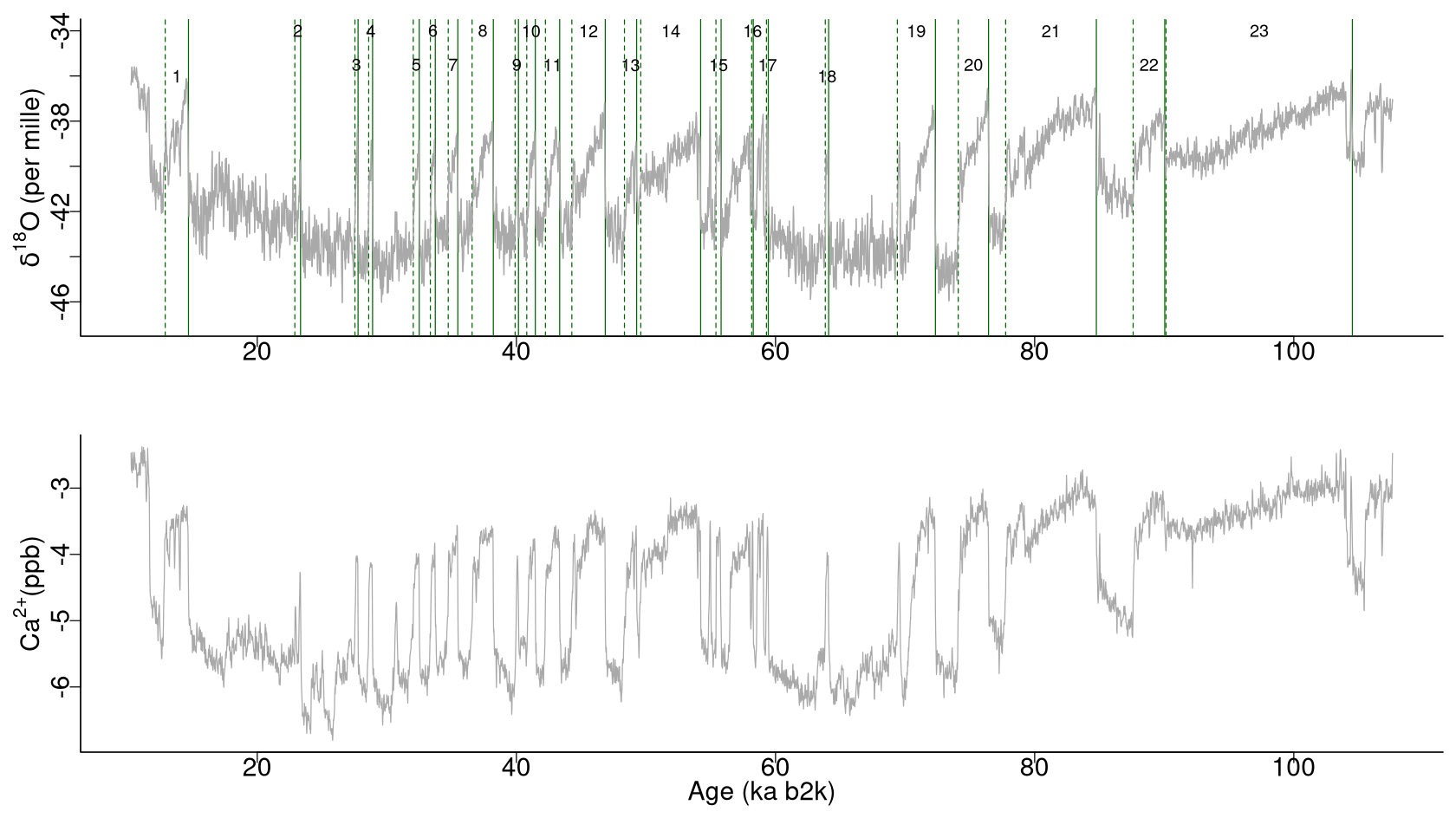
Figure 1Time series of δ18O and Ca2+ concentrations on the GICC05modelext timescale. Note that Ca2+ is on the inverse logarithmic scale. The vertical solid and dashed lines represent, respectively, the start and end times of canonical DO events (Dansgaard et al., 1993; Rasmussen et al., 2014).
The results of the matrix profile analysis of the palaeoclimate time series are presented initially in terms of the characterisation of DO events from a single time series, the δ18O Greenland record, in Sect. 4.1, and the Ca2+ record, in Sect. 4.2. Subsequently, the joint analysis of DO events from multiple time series is documented in Sect. 4.3 using both the δ18O and Ca2+ proxy records.
4.1 Matrix profile analysis of the δ18O record
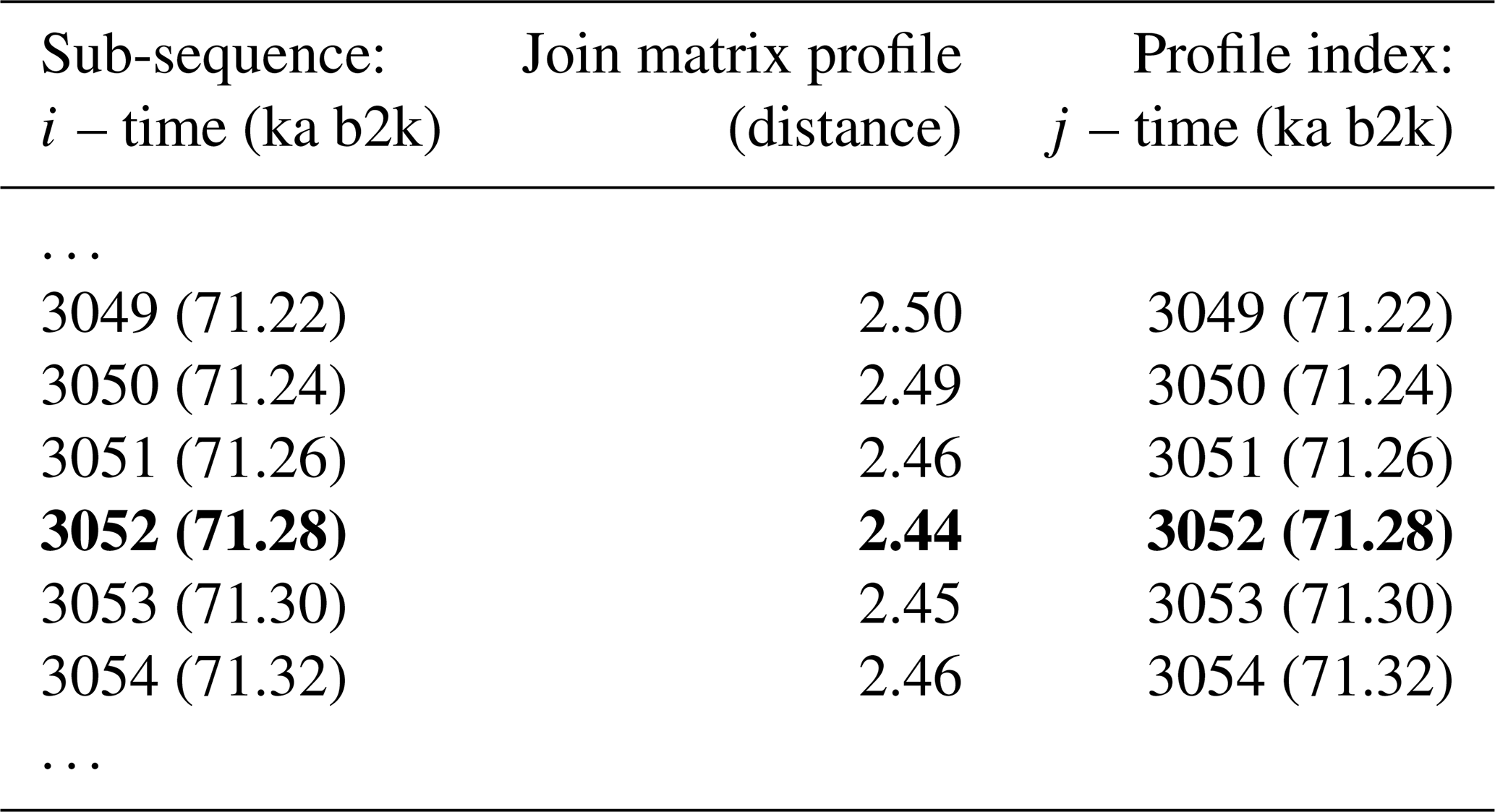
The matrix profile of the δ18O time series is computed using the stomp (Scalable Time series Ordered-search Matrix Profile) algorithm (Zhu et al., 2016) with a sub-sequence length (window size m) of 2500 years (125 data points). The exclusion zone , defined as a proportion of the sub-sequence length, is set to 1, which is equal to the size of the sub-sequence length, in order to exclude trivial matches (similarity of a sub-sequence to another sub-sequence with data values in common). For each ith sub-sequence consisting of the time series values from i to with , its z-normalised Euclidean distance to every other jth sub-sequence is computed. The matrix profile is defined as the smallest value from that set of distances, while the profile index records the location of the most similar (non-trivial) sub-sequence, or in other words the value of j. Table 1 provides an illustrative example of the matrix profile and the corresponding profile index computed for the δ18O time series. The first column contains the data point corresponding to the start of the sub-sequence, i.e. the 3044th value of the time series (and the corresponding time) and so forth. The middle column contains the matrix profile, i.e. the minimum value of all the distances between sub-sequence 3044 and all other sub-sequences in the time series. The third column gives the profile index, which for the first row indicates that the most similar sub-sequence to sub-sequence 3044 is the sub-sequence starting at the 3250th value of the time series – all other sub-sequences in the time series are separated from sub-sequence 3044 by a value higher than 2.37.
Table 1Snippet of the matrix profile and profile index of the δ18O time series. Values corresponding to the global minimum of the matrix profile are represented in bold.
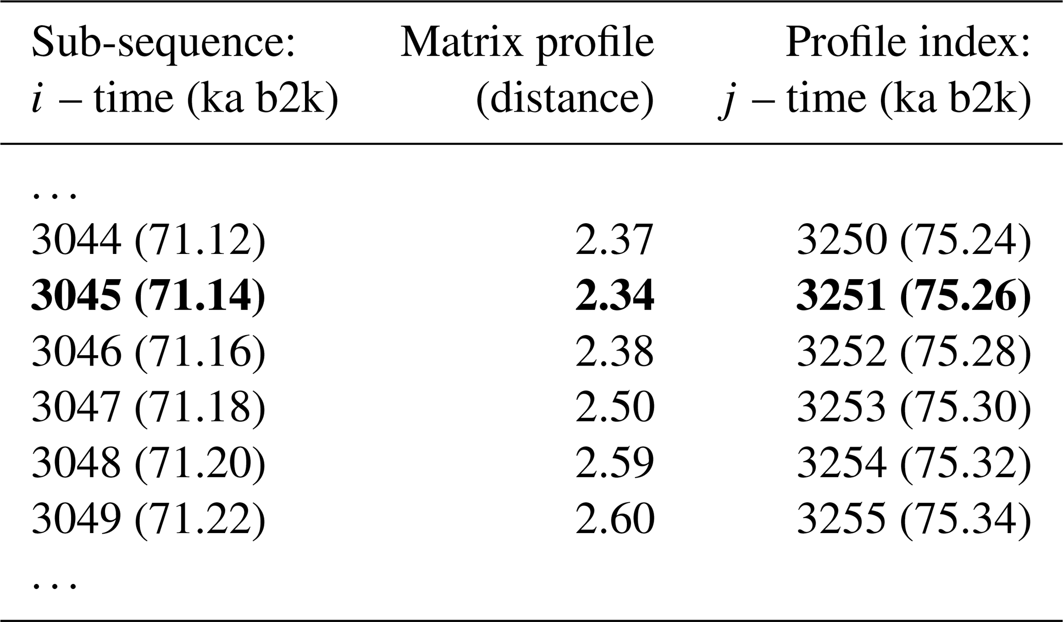
Figure 2 depicts the complete matrix profile for the δ18O time series, which represents the distance of each sub-sequence to its most similar (non-trivial) sub-sequence (same as the middle column in Table 1). The global minimum value of the matrix profile is 2.34, occurring at 71.14 ka (indicated by the vertical dashed line in Fig. 2 and the bold numbers in Table 1). Of all the sub-sequences in the δ18O time series, the one starting at 71.14 ka exhibits the shortest distance to its most similar sub-sequence, i.e. the one starting at 75.26 ka (Table 1). It should be noted that this sub-sequence does not necessarily correspond to the next minimum value of the matrix profile. Rather, it is the sub-sequence that is most similar to the one extracted from the global minimum and not necessarily the sub-sequence with the second-lowest matrix profile distance.
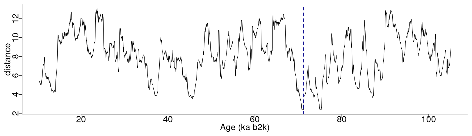
Figure 2Matrix profile of the NGRIP δ18O time series using a window size of 2500 years (125 data points). The dashed vertical line indicates the minimum value of the matrix profile corresponding to the top motif: same age model as in Fig. 1.
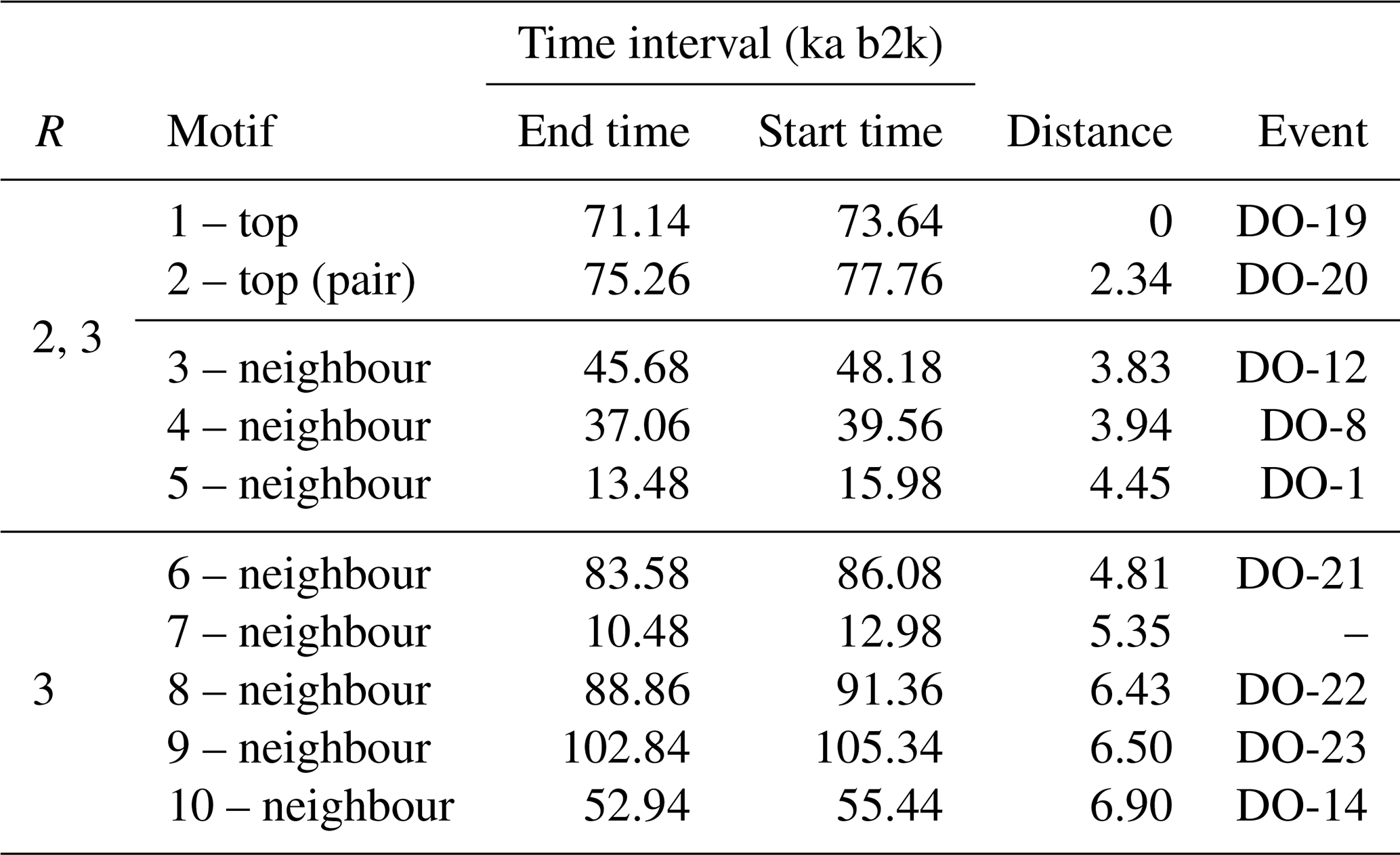
The top motif pair, representing the two most similar sub-sequences in the time series starting at 71.14 and 75.26 ka, respectively, is displayed in Fig. 3. This motif pair corresponds to the canonical DO events DO-19 and DO-20, which are most similar to each other. While the sub-sequence starting at 75.26 ka is most similar to the top sub-sequence corresponding to the matrix profile minimum, at 71.14 ka, other sub-sequences, while not the most similar ones, are still not far off. All the sub-sequences for which the distance to the top sub-sequence at 71.14 ka is within R times the distance from the top motif pair can be considered neighbouring motifs. Table 2 presents the motifs obtained for the δ18O time series using values of R equal to 2 and 3. Setting a value of R=2 enables the extraction of three neighbour motifs to the top motif, while setting R=3 allows for the additional extraction of five further neighbours. It should be noted that the distance represented in Table 2 is the distance of the motif sub-sequence to the top motif and not its matrix profile distance. An alternative approach to the use of a fixed value of the parameter R is to set a maximum distance between a neighbour motif and the main motif based on the variability of the matrix profile. In this study, neighbouring motifs are considered to be separated by less than twice the global standard deviation of the matrix profile (equal to ), which in this case corresponds to the neighbours that would be extracted by considering R=2 (Fig. 3). This aspect of selecting neighbour sequences to the main motif is further discussed in Sect. 5. The last column of Table 2 indicates the canonical DO event that coincides with each motif. The seventh motif (12.98–10.48 ka) does not correspond to a DO event, but it does include the Younger Dryas cooling event (GS-1) and the transition to the Holocene.
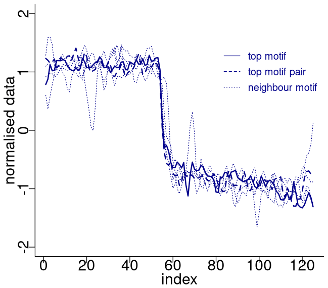
Figure 4 depicts the normalised sub-sequences corresponding to the motifs extracted from the δ18O time series. The top motif represents the patterns corresponding to the canonical DO-19 and DO-20. These aforementioned sub-sequences and their neighbour motifs represent abrupt transitions to warmer conditions, preceded by an approximately stable stadial level and followed by a slow decrease towards stadial conditions.
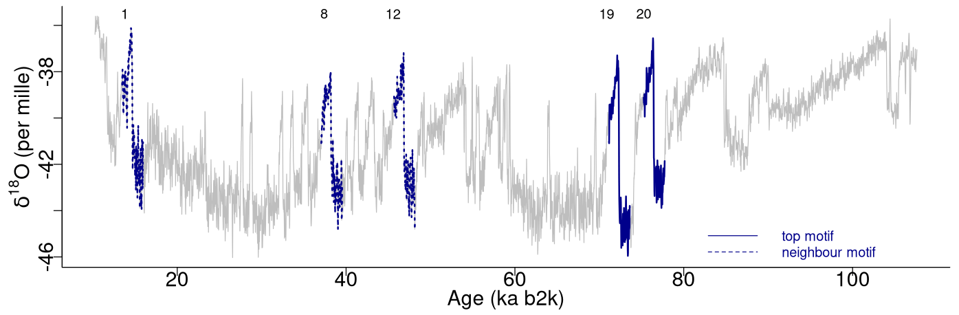
Figure 3Top motifs for the NGRIP δ18O time series and neighbour motifs. The horizontal top numbers indicate the canonical DO events: same age model as in Fig. 1.
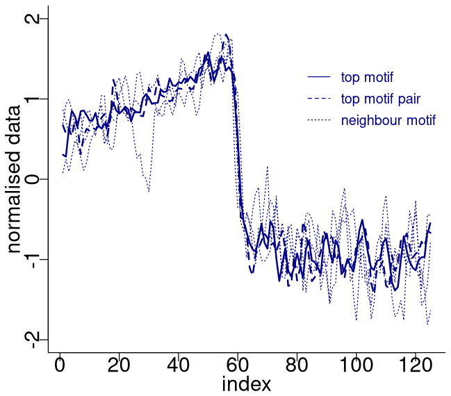
Figure 4Normalised motifs for the NGRIP δ18O time series. The index is the order of the δ18O values in each sub-sequence of 125 values (2500 years). The top motif pair corresponds to DO-19 and DO-20, and the neighbour motif corresponds to DO-12, DO-8, and DO-1.
Table 2Motifs extracted from the matrix profile of the δ18O time series using a window size of 2500 years. The columns display the value of the radius parameter R for neighbouring sub-sequences, the type of motif, the end and start times of the motif, the distance to the top motif, and the corresponding canonical DO event.
4.2 Matrix profile analysis of the Ca2+ record
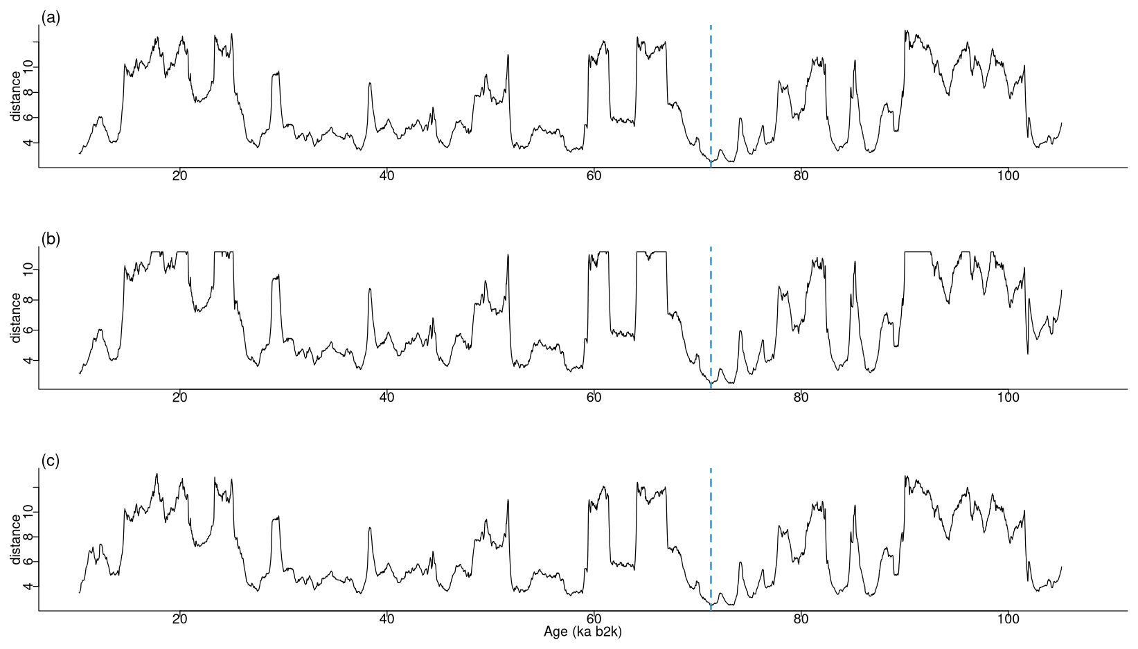
A comparable analysis is conducted for the Ca2+ record employing the same methodology as that employed for the δ18O time series. Figure 5 depicts the matrix profile for the Ca2+ record. While the overall pattern of the Ca2+ series is similar to that of the matrix profile of the δ18O record in Fig. 2, the peaks are sharper due to the lower noise level of the Ca2+ series. Moreover, the minimum value of the matrix profile for the Ca2+ series, indicated by the vertical dashed line in Fig. 5, occurs at a different time (at 37.14 ka) than for δ18O. Consequently, the sub-sequence with the shortest distance to its most similar sub-sequence in the Ca2+ record starts at 37.14 ka, corresponding to DO-8. From the profile index, the most similar sub-sequence, which constitutes the top motif pair for the Ca2+ time series, starts at 45.78 ka, corresponding to DO-12. The aforementioned top motif and its neighbour motifs are summarised in Table 3. The criterion of selecting as neighbour motifs the sub-sequences separated from the main motif by less than twice the matrix profile's standard deviation () yields all neighbour motifs for a radius of R=2 and the first neighbour motif for a value of R=3. This is illustrated in Fig. 6.
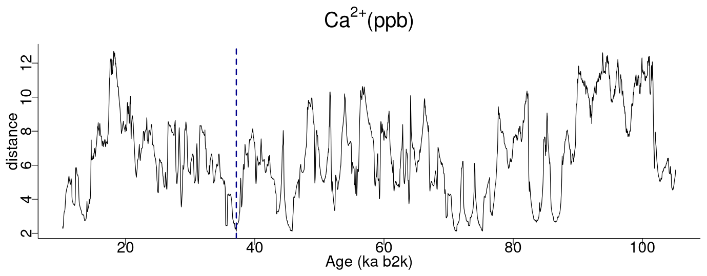
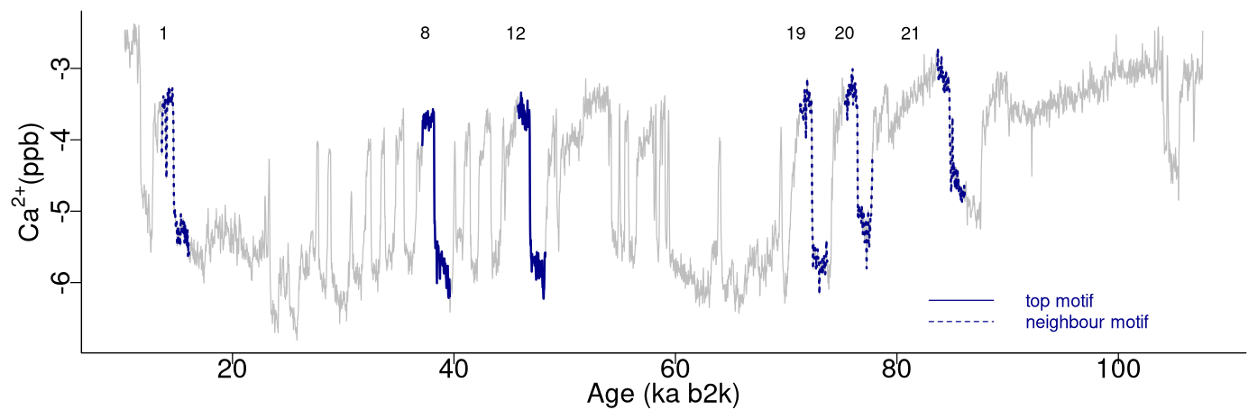
Table 3Motifs extracted from the matrix profile of the Ca2+ record: same conventions as in Table 2.
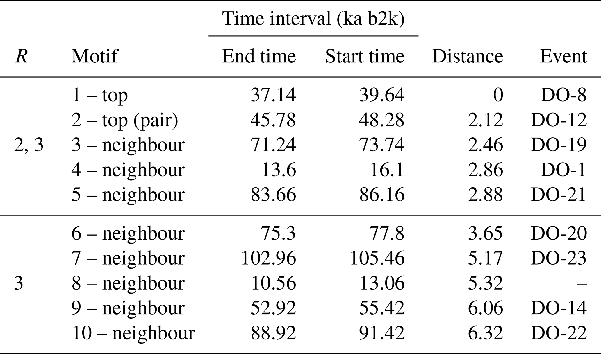
Figure 7 displays the normalised motifs for the Ca2+ time series. These motifs correspond to the same canonical DOs as the motifs of the δ18O time series, with the addition of DO-21. However, the ordering of the motifs differs. In the case of the Ca2+ record, considered on the reverse logarithmic scale, the recurring patterns, constituted by the top motif and its neighbour motifs, represent abrupt decreases in the atmospheric dust concentration. These decreases are preceded by slightly decreasing stadial normalised values and are followed by an approximately stable interstadial level.
4.3 Join matrix profile analysis of the δ18 and Ca2+ records
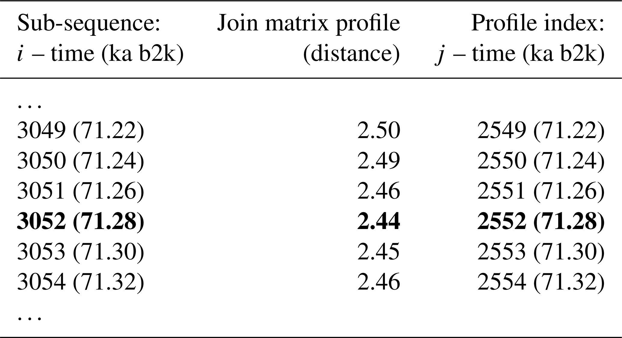
Figure 8 depicts the join matrix profile of the δ18O and Ca2+ time series, which is defined as the distance between each sub-sequence in the δ18O record and its most similar sub-sequence in the Ca2+ record. In this join case, the necessity for an exclusion zone to avoid trivial matches is negated by the fact that the sub-sequences originate from different time series. The join matrix profile (Fig. 8) differs from the previously defined individual profiles but exhibits similarities to the matrix profile for the single δ18O time series (Fig. 2). This is not unexpected given that the temporal variability of the Ca2+ series closely follows that of the δ18O series. For illustrative purposes, a snippet of the join matrix profile and the profile index is presented in Table 4.
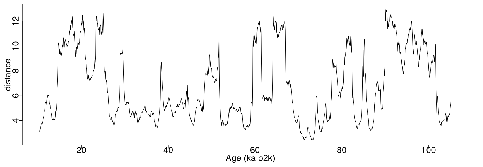
Figure 8Join matrix profile for the δ18O and Ca2+ time series using a window size of 2500 years (125 data points). The dashed vertical line indicates the minimum value of the matrix profile corresponding to the top motif (sub-sequence of the δ18O time series most similar to a sub-sequence in the Ca2+ time series). Same age model than in Fig. 1.
Table 4Snippet of the join matrix profile and the profile index of the δ18O and Ca2+ time series. Values corresponding to the global minimum of the matrix profile are represented in bold.
The minimum value of the join matrix profile indicates the location of the top motif, i.e. the sub-sequence in the δ18O time series which is most similar (distance-wise) to a sub-sequence in the Ca2+ time series (whatever it is). The global minimum of the join matrix profile occurs at 71.28 ka, which is in close proximity to the previously defined minimum for δ18O at 71.14 ka. Table 4 indicates that the sub-sequence in the δ18O time series starting at 71.28 ka exhibits the greatest similarity to the sub-sequence in the Ca2+ record also starting at 71.28 ka. The most analogous sub-sequences across the δ18O and Ca2+ records are presented in Fig. 9, still with Ca2+ displayed on the reverse logarithmic scale. In this particular case, the location (time) of the top motif is the same for the two records, and thus normalised motifs are represented on the temporal scale rather than plotted as a function of the index value from m=1 to m=125, as in Figs. 4 and 7. This motif is identical to the previously identified motif in the individual analysis of the δ18O time series (Sect. 4.1). This transition, occurring approximately 70 000 years ago (the canonical DO-19), exhibits the most analogous patterns of warming and cooling across δ18O and less dusty or dustier Ca2+ records. Additionally, it bears the closest resemblance in shape to the transition in the δ18O record immediately after, approximately 73 000 years ago.
While the matrix profile is an algorithmic approach that enables the extraction of recurring patterns in a time series, its results are dependent on parameters that are prescribed empirically, often through a trial-and-error process, and they are dependent on the specific application and purpose of the analysis. These constraints are discussed in Sect. 5.1, while Sect. 5.2 discusses the extraction of the most similar pattern across two time series. In the case of short time series, such as the ones analysed here, the utility of the matrix profile approach is more obvious when applied to two time series. However, finding motifs in a single long and high-frequency time series is a very common need in data-mining contexts, for which the matrix profile of a single time series is considered to be an extremely useful tool (Zhu et al., 2020).
5.1 Matrix profile parameters
The matrix profile is dependent on a single parameter, the sub-sequence length m. Consequently, it is a method that can be readily applied to any time series, as it only requires the appropriate specification of a window size (see Sect. 4.1). However, the matrix profile results are highly contingent upon the value selected for m. There are no universal formulas or rigorous criteria for selecting the window size, as this depends on the objective of the analysis and the type of motif being investigated. The sub-sequence length is typically determined by considering the length of the patterns of interest in the time series being analysed. In the absence of prior knowledge regarding the length of the motif of interest in a time series, an extension of the matrix profile, which computes nearest-neighbour information for all sub-sequences of all lengths, can be considered (Madrid et al., 2019).
In our study, a window size of 2500 years was selected as adequate for the extraction of motifs with durations typical of DO events. The matrix profile obtained with this window size is compared in Fig. 10 with the matrix profile for window sizes of 3000 and 3500 years. The matrix profile values increase with increasing values of m, yet the results remain remarkably consistent across this range of window sizes, exhibiting a similar overall pattern and the lowest distance at around 70 ka. The highest values of the matrix profile (at around 90, 66, and 26 ka) reflect the flatter parts of the δ18O time series, which lack discernible features and thus comprise more disparate sub-sequences. The motifs obtained for the different window sizes are presented in Fig. 11, which provides further evidence of the robustness of the recurring patterns extracted in the considered window range.
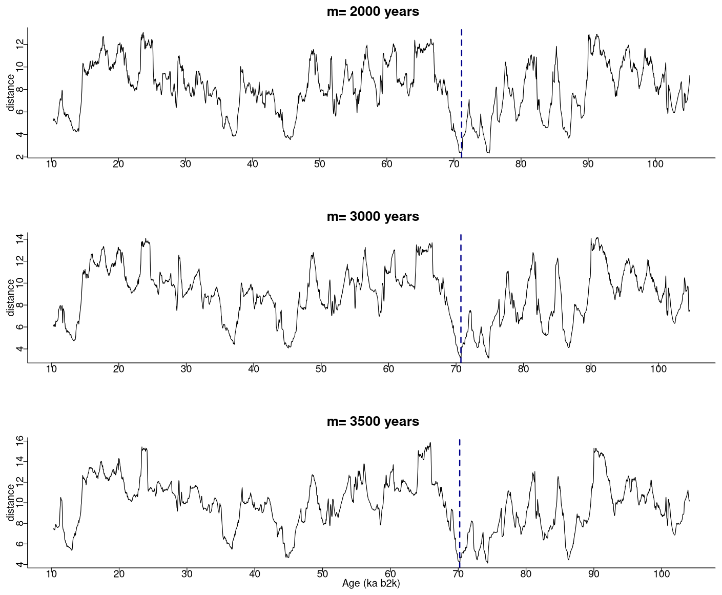
Figure 10Matrix profile of the NGRIP δ18O time series for different window sizes. The dashed vertical line indicates the minimum value of the matrix profile: same age model as in Fig. 1.
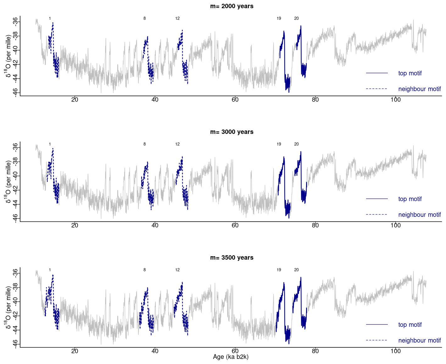
Figure 11Motifs extracted from the matrix profile of the NGRIP δ18O time series for different window sizes: same age model as in Fig. 1.
The top motif is derived directly from the lowest values of the matrix profile and therefore depends only on the specified sub-sequence length. However, the extraction of neighbouring sequences to the top motif and of other motifs depends not only on the window size, but also on the tolerance (distance-wise) with which a sub-sequence is considered to match a pattern given by the value of parameter R. Once more, there are no specific criteria for specifying R, other than it should be a small integer value. The larger the value of R, the greater the distance between sub-sequences considered to match the motif and therefore the lower the similarity between potential matches. The use of smaller values of R reduces the potential for considering as matching sub-sequences that are dissimilar. This is demonstrated in Fig. 12, which depicts the normalised motifs for the NGRIP δ18O time series using R=2 and the supplementary motifs obtained using R=3. To facilitate visualisation, the first two neighbour motifs for R=3 are plotted separately from the subsequent neighbour motifs (see Table 2). The discrepancy between the top motif pattern and the neighbour motifs assigned increases with the higher-order motifs indicating a value of R=3 is not optimal in this case. Notwithstanding, the neighbour motifs 6 and 7, derived from the use of R=3, remain in close proximity to the primary motif. An alternative approach to enhance the flexibility of the extraction of neighbour motifs is to consider a maximum distance calculated not from a radius R but rather from a metric computed from the overall matrix profile variability. In this study we adopt this approach, whereby neighbour motifs are selected as the patterns that are separated from the top motif by less than twice the standard deviation of the matrix profile. For the δ18O time series, the motifs obtained using this criterion are identical to those obtained by setting R=2. However, this approach yields the same neighbour motifs for the Ca2+ time series as for R=2, in addition to the first neighbour motif corresponding to R=3.
The identification of higher-order motifs, other than the top (global) motif corresponding to the matrix profile minimum, is more challenging due to the dependence on the constraints that must be set in terms of the maximum distance for which sub-sequences are taken as matching. As illustrated in the preceding section, varying the radius parameter yields both matching and dissimilar patterns. Therefore, we have adopted a more flexible criterion than the radius parameter R in order to ensure appropriately constrained results and interpretable motifs. While the matrix profile calculation is only dependent on the sub-sequence length and the top motif is objectively obtained from the global minimum value of the matrix profile, subsequent motifs or neighbours depend on the adopted distance constraints. To circumvent this limitation, this study focuses on the extraction of the top motif from the palaeoclimate records. In general, the extraction of motifs has to take into account the purpose of the analysis and is very much problem-dependent in terms of what the patterns of interest are in a time series (which may differ, even for the same time series, depending on the goal of the analysis). In the case of very large datasets for which information on the patterns of interest is not available, the statistical significance of motifs can be assessed to evaluate which additional motifs are significant, other than the top motif (Castro and Azevedo, 2011).
The comparison of sub-sequence similarity is performed here based on the Euclidean distance metric. An alternative would be to consider instead dynamic time warping (DTW) as a more robust distance measure for time series (Keogh and Ratanamahatana, 2005). However, empirical comparisons showed that the Euclidean distance is competitive with or superior to more complex measures (Ding et al., 2008). Therefore, the Euclidean distance between z-normalised sub-sequences is employed as the similarity measure in this study.
Here we only discuss the influence on matrix profile results of methodological options in terms of parameters and metric selection. A further extension would be to assess how differences in the time series data would impact the matrix profile results, e.g. by applying surrogate time series methods such as the approach of Nakamura and Small (2005). Extending the methodology to account for uncertainty in dating and proxy values would be a further methodological extension particularly relevant for palaeoclimate time series.
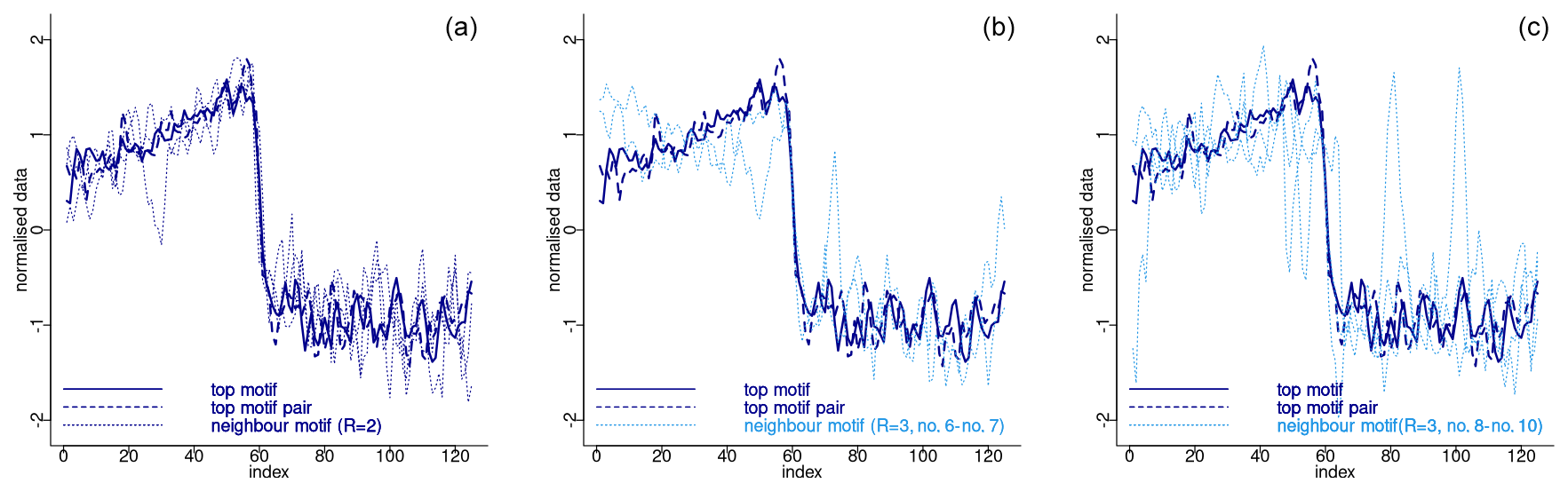
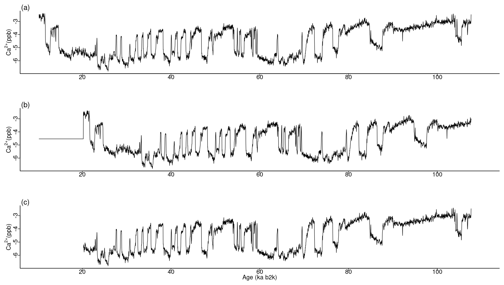
Figure 13Various time series of Ca2+ concentration. (a) Original values, (b) version shifted by 10 ka with the same size, and (c) version trimmed by 10 ka with a smaller size: same age model as in Fig. 1.
5.2 Extraction of the dominant motif across the two time series
The most analogous pattern (top motif) across two time series does not need to occur at the same time in the two series. This fact is illustrated by considering the same δ18O and Ca2+ proxy records but artificially changing the Ca2+ time series in two distinct ways. The first case introduces an artificial shift in time of 500 data points (10 ka) by adding to the beginning of the record 500 points with the same value as the mean of the Ca2+ time series. The second case removes the first 500 data points of the Ca2+ series, thus obtaining a shorter record of a different length than the δ18O series. The time series are displayed in Fig. 13, and the join matrix profile between the δ18O series and these versions of the Ca2+ series is presented in Fig. 14. The outcomes are largely analogous, with only minor discrepancies in the join matrix profile for the different versions of the Ca2+ time series. In the case of the shifted version of the Ca2+ series (Fig. 14b), the difference between this version and the original is observed in the highest values of the join matrix profile, which are flatter. The matrix profile peaks correspond to parts of the series with no discernible temporal structure, typically a featureless noise level. In such cases the most similar sub-sequences are the stable level values (equal to the mean of the time series) that were introduced at the beginning of the record. In the case of the trimmed version of the Ca2+ series (Fig. 14c), it should be noted that the join matrix profile has the same length, despite the reduced length of the Ca2+ series. This is because the join matrix profile contains the distance of every sub-sequence in the δ18O series to the trimmed Ca2+ series (of a smaller size). Consequently, the number of sub-sequences (in the δ18O series) remains constant, yet the distances are calculated between each of these sub-sequences and a smaller number of sub-sequences in the Ca2+ series. The principal distinction between the join matrix profile values in this particular case is observed at the beginning of the record, as the initial sub-sequences of the δ18O series are most similar to the initial sub-sequences in the Ca2+ series, which no longer exist, having been matched to other sub-sequences in the Ca2+ time series.
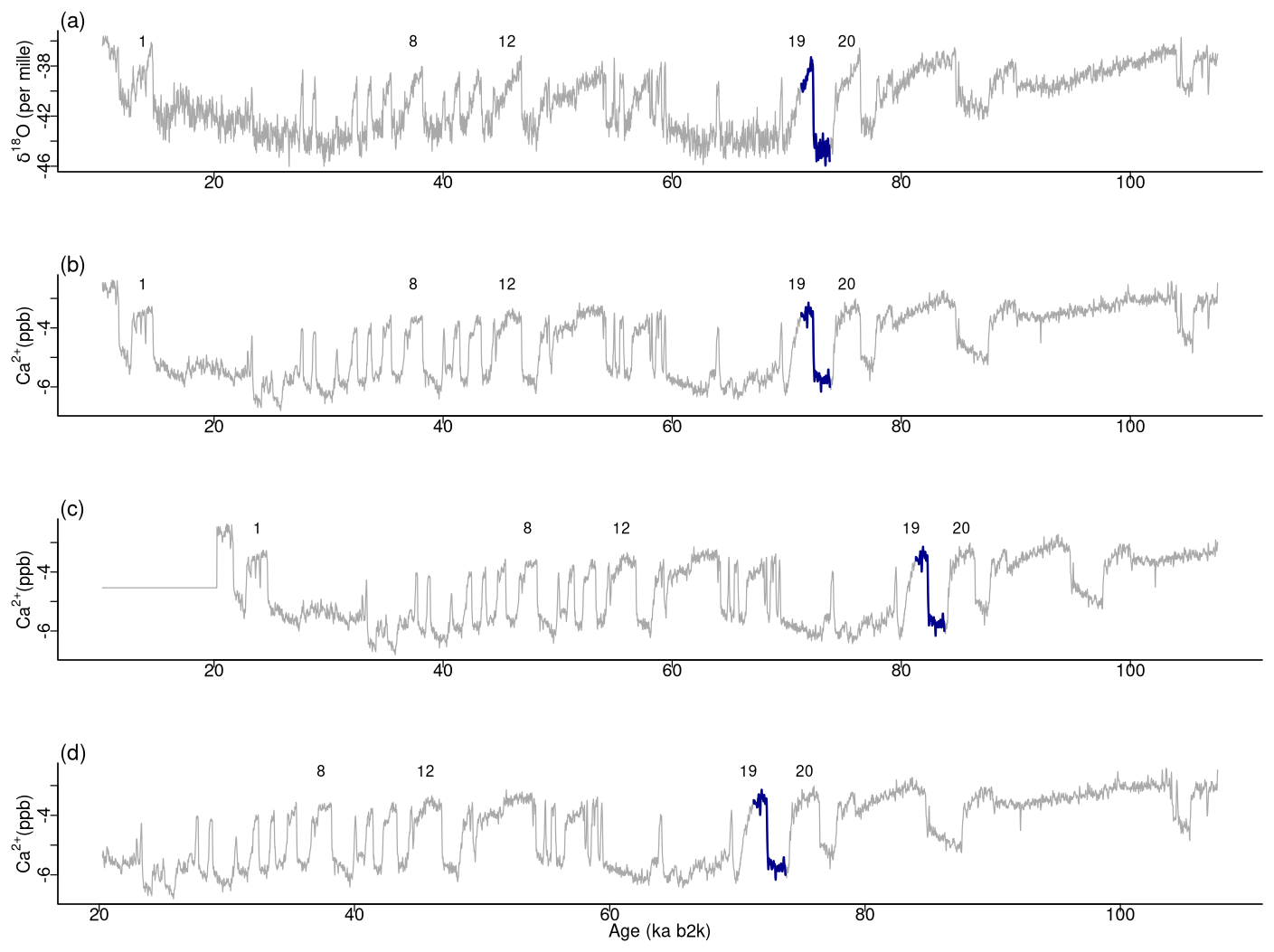
Figure 15Top motif across δ18O and the Ca2+ time series. (a) δ18O record, (b) original Ca2+ time series, (c) shifted version, and (d) trimmed version: same age model as in Fig. 1.
For the original version and the two versions of Ca2+ under consideration, the minimum value of the join matrix profile occurs at the same time corresponding to the top motif previously identified in the δ18O record at around 71 ka. Tables 5 and 6 present excerpts of the join matrix profile and profile index for the shifted and trimmed Ca2+ time series, respectively. In the former case, the minimum value of the matrix profile occurs at the same index value of the δ18O time series as previously defined. However, the most similar sub-sequence in the Ca2+ record is no longer coincidental, although it is correctly identified at 10 ka later. A comparable outcome is observed in the latter case. The profile index indicates that the most similar sub-sequence occurs at the index value of the time series corresponding to the correct time. Figure 15 displays the top motif across the δ18O time series and the different versions of the Ca2+ series. It can be seen that the most similar sub-sequence across the two records corresponds to the canonical DO-19. Furthermore, the same results are obtained with shifted and trimmed versions of the Ca2+ time series, demonstrating the robustness of the approach.
Table 5Snippet of the matrix profile and profile index for the shifted Ca2+ time series: same convention as for Table 4.
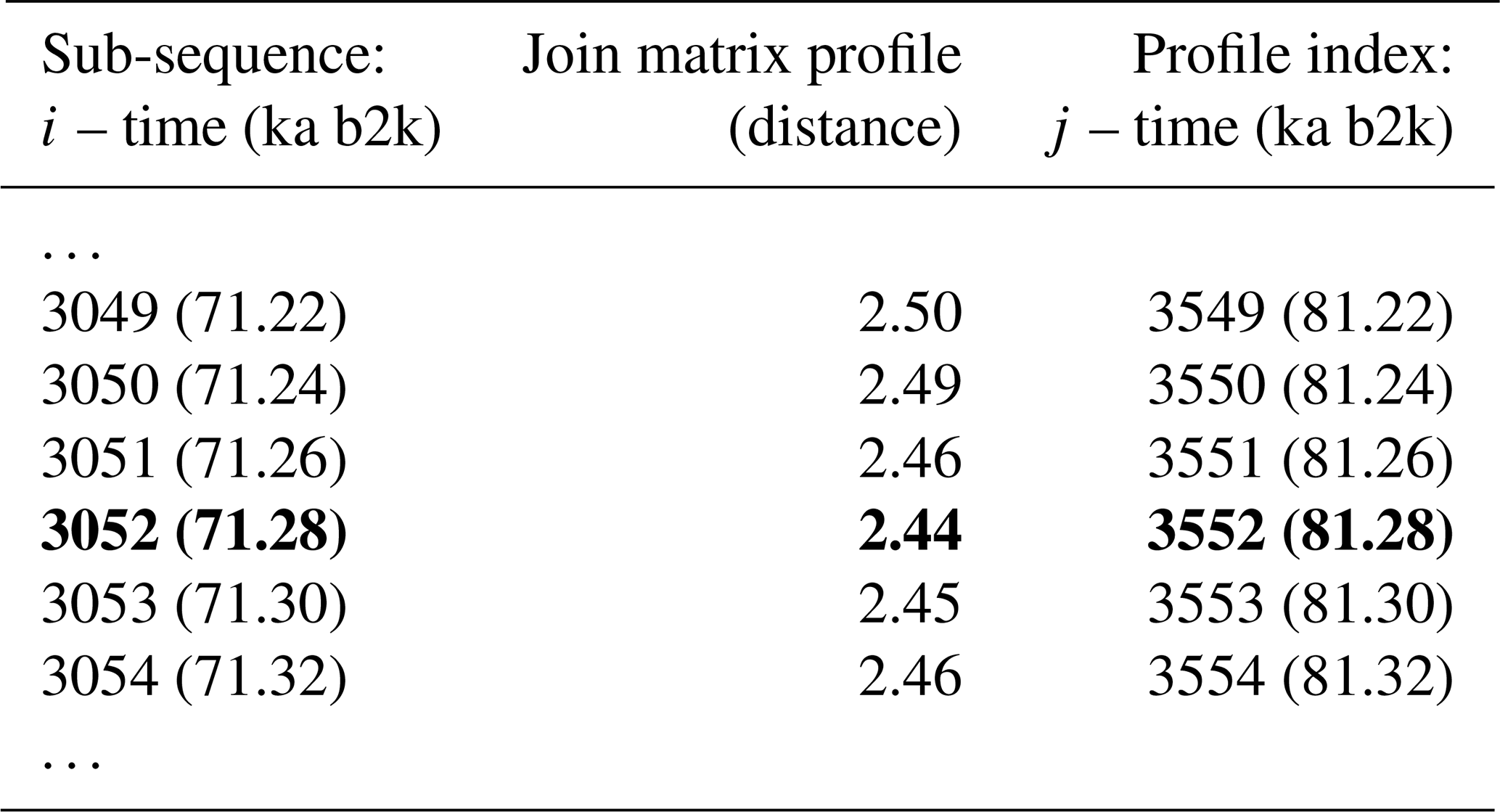
Table 6Snippet of the matrix profile and profile index for the trimmed Ca2+ time series: same convention as for Table 4.
In this study, the algorithmic matrix profile approach was employed to identify recurring patterns in the well-studied NGRIP palaeoclimate record. The matrix profile is dependent on a single parameter, the sub-sequence length. This is generally set by considering the typical duration of the patterns of interest, as there are no stringent criteria for its specification. In this analysis, a window size of 2500 years was considered. Shorter patterns exist in the time series and are of interest, but short-length sub-sequences can be harder to identify in terms of recurring patterns, and thus this study focused on patterns spanning around 2500 years. Consistent patterns were obtained for window sizes of 3000 and 3500 years, indicating that the results are robust to window sizes within this range.
The objective of the matrix profile approach was not to identify the abrupt DO transitions or to determine their precise timing. Rather, the objective was to characterise the abrupt transitions in a purely data-driven manner, based on the shape of the corresponding DO patterns. For the δ18O time series, the transitions corresponding to the canonical events DO-19 and DO-20, occurring at around 72 and 76 ka, respectively, are identified as the most similar ones. These form the most prominent top motif pair in the time series, indicating that analogous mechanisms may have been responsible for these abrupt climate transitions. Further transitions corresponding to the DO-12, DO-8, and DO-1 events are established as neighbouring transitions, with a similar shape characterised by an abrupt transition to warm conditions, preceded by approximately stable stadial conditions and followed by a slow return to cold conditions. The same transitions are identified in the Ca2+ time series, but their ordering differs. The transitions corresponding to events DO-8 and DO-12 are identified as the most similar ones in the Ca2+ record. These events are distinguished by an abrupt decrease in the terrestrial dust concentration, followed by a period of stable dust conditions.
The matrix profile method has also been employed to identify the most analogous pattern across the two different δ18O and Ca2+ time series, despite their disparate lengths. Given the high degree of similarity between the two records, the assumption of their simultaneous change, within the 20-year resolution of the records, serves as the basis for the definition of stratigraphic events in Rasmussen et al. (2014). The join matrix profile identifies a coincident top motif, which also corresponds to the DO-19 canonical event. When considering a shifted version of the Ca2+ timescale, the join matrix profile is able to identify the same sub-sequence as the most similar pattern across the two time series, though they are not coincident in time. This allows for accurate identification of the time shift that was introduced. A shorter version of the Ca2+ time series also demonstrates the ability of the join matrix profile to correctly identify matching patterns across the δ18O and Ca2+ records. This indicates the potential of the join matrix profile as an objective quantitative approach for matching palaeoclimate time series as an alternative to visual wiggle matching. The identification of similarities in events across distinct proxy records can assist the investigation of the key factors affecting the marine (δ18O) and continental (dust) hydrological cycles during the last 130 000 years. This can be tested by Earth system models.
All the data and software code used in this work are publicly available at https://doi.org/10.25747/T9GX-9729 (Barbosa et al., 2024).
SB: conceptualisation; formal analysis; writing – original draft preparation. MES: writing – review and editing. DDR: writing – review and editing.
The contact author has declared that none of the authors has any competing interests.
Publisher's note: Copernicus Publications remains neutral with regard to jurisdictional claims made in the text, published maps, institutional affiliations, or any other geographical representation in this paper. While Copernicus Publications makes every effort to include appropriate place names, the final responsibility lies with the authors.
This work is TiPES contribution no. 281.
This research has been supported by the European Union's Horizon 2020 research and innovation programme (grant no. 820970) and the Fundação para a Ciência e a Tecnologia (grant no. LA/P/0063/2020).
This paper was edited by Kira Rehfeld and reviewed by two anonymous referees.
Agrawal, R., Faloutsos, C., and Swami, A.: Efficient similarity search in sequence databases, in: Foundations of Data Organization and Algorithms: 4th International Conference, FODO'93 Chicago, Illinois, USA, October 13–15, 1993 Proceedings 4, 69–84, Springer, https://doi.org/10.1007/3-540-57301-1_5, 1993. a
Andersen, K. K., Azuma, N., Barnola, J.-M., Bigler, M., Biscaye, P., Caillon, N., Chappellaz, J., Clausen, H. B., Dahl-Jensen, D., Fischer, H., Flückiger, J., Fritzsche, D., Fujii, Y., Goto-Azuma, K., Grønvold, K., Gundestrup, N. S., Hansson, M., Huber, C., Hvidberg, C. S., Johnsen, S. J., Jonsell, U., Jouzel, J., Kipfstuhl, S., Landais, A., Leuenberger, M., Lorrain, R., Masson-Delmotte, V., Miller, H., Motoyama, H., Narita, H., Popp, T., Rasmussen, S. O., Raynaud, D., Rothlisberger, R., Ruth, U., Samyn, D., Schwander, J., Shoji, H., Siggard-Andersen, M.-L., Steffensen, J. P., Stocker, T., Sveinbjörnsdóttir, A. E., Svensson, A., Takata, M., Tison, J.-L., Thorsteinsson, T., Watanabe, O., Wilhelms, F., and White, J. W. C.: High-resolution record of Northern Hemisphere climate extending into the last interglacial period, Nature, 431, 147–151, https://doi.org/10.1038/nature02805, 2004. a
Bagniewski, W., Ghil, M., and Rousseau, D. D.: Automatic detection of abrupt transitions in paleoclimate records, Chaos, 31, 113129, https://doi.org/10.1063/5.0062543, 2021. a, b
Bagniewski, W., Rousseau, D.-D., and Ghil, M.: The PaleoJump database for abrupt transitions in past climates, Sci. Rep., 13, 4472, https://doi.org/10.1038/s41598-023-30592-1, 2023. a
Barbosa, S., Silva, M., and Rousseau, D.-D.: Matrix profile analysis of Dansgaard-Oeschger events in palaeoclimate time series, INESC TEC [data set], https://doi.org/10.25747/T9GX-9729, 2024. a
Castro, N. and Azevedo, P. J.: Time Series Motifs Statistical Significance, 687–698, https://doi.org/10.1137/1.9781611972818.59, 2011. a
Corrick, E. C., Drysdale, R. N., Hellstrom, J. C., Capron, E., Rasmussen, S. O., Zhang, X., Fleitmann, D., Couchoud, I., and Wolff, E.: Synchronous timing of abrupt climate changes during the last glacial period, Science, 369, 963–969, https://doi.org/10.1126/science.aay5538, 2020. a
Dansgaard, W., Clausen, H. B., Gundestrup, N., Hammer, C. U., Johnsen, S. F., Kristinsdottir, P., and Reeh, N.: A new Greenland deep ice core, Science, 218, 1273–1277, https://doi.org/10.1126/science.218.4579.1273, 1982. a
Dansgaard, W., Johnsen, S. J., Clausen, H. B., Dahl-Jensen, D., Gundestrup, N. S., Hammer, C. U., Hvidberg, C. S., Steffensen, J. P., Sveinbjörnsdottir, A., Jouzel, J., and Bond, G.: Evidence for general instability of past climate from a 250-kyr ice-core record, Nature, 364, 218–220, https://doi.org/10.1038/364218a0, 1993. a
Ding, H., Trajcevski, G., Scheuermann, P., Wang, X., and Keogh, E.: Querying and mining of time series data: experimental comparison of representations and distance measures, Proc. VLDB Endowment, 1, 1542–1552, https://doi.org/10.14778/1454159.1454226, 2008. a
Fischer, H., Fundel, F., Ruth, U., Twarloh, B., Wegner, A., Udisti, R., Becagli, S., Castellano, E., Morganti, A., Severi, M., Wolff, E., Littot. G., Röthlisberger, R., Mulvaney, R., Hutterli, M., Kaufmann, P., Federer, U., Lambert, F., Bigler, M., Hansson, M., Jonsell, U., de Angelis, M., Boutron, C., Siggaard-Andersen, M.-L., Steffensen, J. P., Barbante, C., Gaspari, V., Gabrielli, P., and Wagenbach, D.: Reconstruction of millennial changes in dust emission, transport and regional sea ice coverage using the deep EPICA ice cores from the Atlantic and Indian Ocean sector of Antarctica, Earth Planet. Sc. Lett., 260, 340–354, https://doi.org/10.1016/j.epsl.2007.06.014, 2007. a
Fuhrer, K., Wolff, E. W., and Johnsen, S. J.: Timescales for dust variability in the Greenland Ice Core Project (GRIP) ice core in the last 100,000 years, J. Geophys. Res-Atmos., 104, 31043–31052, https://doi.org/10.1029/1999JD900929, 1999. a
Held, F., Cheng, H., Edwards, R., Tüysüz, O., Koç, K., and Fleitmann, D.: Dansgaard-Oeschger cycles of the penultimate and last glacial period recorded in stalagmites from Türkiye, Nat. Commun., 15, 1183, https://doi.org/10.1038/s41467-024-45507-5, 2024. a
Johnsen, S., Clausen, H., Dansgaard, W., Fuhrer, K., Gundestrup, N., Hammer, C., Iversen, P., Jouzel, J., Stauffer, B., and Steffensen, J.: Irregular glacial interstadials recorded in a new Greenland ice core, Nature, 359, 311–313, https://doi.org/10.1038/359311a0, 1992. a
Keogh, E. and Ratanamahatana, C. A.: Exact indexing of dynamic time warping, Knowl. Inf. Syst., 7, 358–386, https://doi.org/10.1007/s10115-004-0154-9, 2005. a
Kindler, P., Guillevic, M., Baumgartner, M., Schwander, J., Landais, A., and Leuenberger, M.: Temperature reconstruction from 10 to 120 kyr b2k from the NGRIP ice core, Clim. Past, 10, 887–902, https://doi.org/10.5194/cp-10-887-2014, 2014. a
Lauterbach, S., Brauer, A., Andersen, N., Danielopol, D. L., Dulski, P., Hüls, M., Milecka, K., Namiotko, T., Obremska, M., Von Grafenstein, U., and Participants, D.: Environmental responses to Lateglacial climatic fluctuations recorded in the sediments of pre-Alpine Lake Mondsee (northeastern Alps), J. Quaternary Sci., 26, 253–267, https://doi.org/10.1002/jqs.1448, 2011. a
Law, S. M.: STUMPY: A Powerful and Scalable Python Library for Time Series Data Mining, The Journal of Open Source Software, 4, 1504, https://doi.org/10.21105/joss.01504, 2019. a
Lin, J., Keogh, E., Patel, P., and Lonardi, S.: Finding Motifs in Time Series, in: 6ACM SIGKDD'02, SIGKDD '02, 23–26 July 2002, Edmonton, Alberta, Canada, 23–26, https://cs.gmu.edu/~jessica/publications/motif_tdm02.pdf (last access: 10 May 2024), 2002. a
Lohmann, J.: Prediction of Dansgaard-Oeschger Events From Greenland Dust Records, Geophys. Res. Lett., 46, 12427–12434, https://doi.org/10.1029/2019GL085133, 2019. a
Lohmann, J. and Ditlevsen, P. D.: Objective extraction and analysis of statistical features of Dansgaard–Oeschger events, Clim. Past, 15, 1771–1792, https://doi.org/10.5194/cp-15-1771-2019, 2019. a
Madrid, F., Imani, S., Mercer, R., Zimmerman, Z., Shakibay, N., and Keogh, E.: Matrix profile xx: Finding and visualizing time series motifs of all lengths using the matrix profile, in: 2019 IEEE ICBK, 175–182, https://doi.org/10.1109/ICBK.2019.00031, 2019. a
Marwan, N., Romano, M. C., Thiel, M., and Kurths, J.: Recurrence plots for the analysis of complex systems, Phys. Rep., 438, 237–329, https://doi.org/10.1016/j.physrep.2006.11.001, 2007. a
Marwan, N., Schinkel, S., and Kurths, J.: Recurrence plots 25 years later – Gaining confidence in dynamical transitions, Europhys. Lett., 101, 20007, https://doi.org/10.1209/0295-5075/101/20007, 2013. a
Mueen, A., Keogh, E., Zhu, Q., Cash, S., and Westover, B.: Exact discovery of time series motifs, in: Proc. SIAM International conference on data mining, 30 April–2 May 2009, Sparks, Nevada, 473–484, https://doi.org/10.1137/1.9781611972795.41, 2009. a
Nakamura, T. and Small, M.: Small-shuffle surrogate data: Testing for dynamics in fluctuating data with trends, Phys. Rev. E, 72, 056216, https://doi.org/10.1103/PhysRevE.72.056216, 2005. a
Peterson, L. C., Haug, G. H., Hughen, K. A., and Rohl, U.: Rapid changes in the hydrologic cycle of the tropical Atlantic during the last glacial, Science, 290, 1947–1951, https://doi.org/10.1126/science.290.5498.1947, 2000. a
R Core Team: R: A Language and Environment for Statistical Computing, R Foundation for Statistical Computing, Vienna, Austria, https://www.R-project.org/ (last access: 12 May 2024), 2022. a
Rasmussen, S. O., Bigler, M., Blockley, S. P., Blunier, T., Buchardt, S. L., Clausen, H. B., Cvijanovic, I., Dahl-Jensen, D., Johnsen, S. J., Fischer, H., Gkinis, V., Guillevic, M., Hoek, W. Z., Lowe, J. J., Pedro, J. B., Popp, T., Seierstad, I. K., Steffensen, J. P., Svensson, A. M., Vallelonga, P., Vinther, B. M., Walker, M. J., Wheatley, J. J., and Winstrup, M.: A stratigraphic framework for abrupt climatic changes during the Last Glacial period based on three synchronized Greenland ice-core records: refining and extending the INTIMATE event stratigraphy, Quaternary Sci. Rev., 106, 14–28, https://doi.org/10.1016/j.quascirev.2014.09.007, 2014. a, b, c, d, e, f, g, h
Rousseau, D.-D., Boers, N., Sima, A., Svensson, A., Bigler, M., Lagroix, F., Taylor, S., and Antoine, P.: (MIS3 & 2) millennial oscillations in Greenland dust and Eurasian aeolian records – A paleosol perspective, Quaternary Sci. Rev., 169, 99–113, https://doi.org/10.1016/j.quascirev.2017.05.020, 2017. a, b
Rousseau, D.-D., Bagniewski, W., and Ghil, M.: Abrupt climate changes and the astronomical theory: are they related?, Clim. Past, 18, 249–271, https://doi.org/10.5194/cp-18-249-2022, 2022. a
Rousseau, D.-D., Bagniewski, W., and Cheng, H.: A reliable benchmark of the last 640,000 years millennial climate variability, Sci. Rep., 13, 22851, https://doi.org/10.1038/s41598-023-49115-z, 2023a. a
Rousseau, D.-D., Bagniewski, W., and Lucarini, V.: A punctuated equilibrium analysis of the climate evolution of cenozoic exhibits a hierarchy of abrupt transitions, Sci. Rep., 13, 11290, https://doi.org/10.1038/s41598-023-38454-6, 2023b. a
Seierstad, I. K., Abbott, P. M., Bigler, M., Blunier, T., Bourne, A. J., Brook, E., Buchardt, S. L., Buizert, C., Clausen, H. B., Cook, E., Dahl-Jensen, D., Davies, S. M., Guillevic, M., Johnsen, S. J., Pedersen, D. S., Popp, T. J., Rasmussen, S. O., Severinghaus, J. P., Svensson, A., and Vinther, B. M.: Consistently dated records from the Greenland GRIP, GISP2 and NGRIP ice cores for the past 104 ka reveal regional millennial-scale δ18O gradients with possible Heinrich event imprint, Quaternary Sci. Rev., 106, 29–46, https://doi.org/10.1016/j.quascirev.2014.10.032, 2014. a
Yeh, C.-C. M., Zhu, Y., Ulanova, L., Begum, N., Ding, Y., Dau, H. A., Silva, D. F., Mueen, A., and Keogh, E.: Matrix profile I: all pairs similarity joins for time series: a unifying view that includes motifs, discords and shapelets, in: 2016 IEEE ICDM, 12–15 December 2016, Barcelona, Spain, 1317–1322, https://doi.org/10.1109/ICDM.2016.0179, 2016. a, b
Yeh, C.-C. M., Kavantzas, N., and Keogh, E.: Matrix profile VI: Meaningful multidimensional motif discovery, in: 2017 IEEE ICDM, 18–21 November 2017, New Orleans, LA, USA, 565–574, https://doi.org/10.1109/ICDM.2017.66, 2017. a
Yeh, C.-C. M., Zhu, Y., Ulanova, L., Begum, N., Ding, Y., Dau, H. A., Zimmerman, Z., Silva, D. F., Mueen, A., and Keogh, E.: Time series joins, motifs, discords and shapelets: a unifying view that exploits the matrix profile, Data Min. Knowl. Disc., 32, 83–123, https://doi.org/10.1007/s10618-017-0519-9, 2018. a, b, c
Zhu, Y., Zimmerman, Z., Senobari, N. S., Yeh, C.-C. M., Funning, G., Mueen, A., Brisk, P., and Keogh, E.: Matrix profile II: Exploiting a novel algorithm and gpus to break the one hundred million barrier for time series motifs and joins, in: 2016 IEEE ICDM, 12–15 December 2016, Barcelona, Spain, 739–748, https://doi.org/10.1109/ICDM.2016.0085, 2016. a
Zhu, Y., Gharghabi, S., Silva, D. F., Dau, H. A., Yeh, C.-C. M., Shakibay Senobari, N., Almaslukh, A., Kamgar, K., Zimmerman, Z., Funning, G., Mueen, A., and Keogh, E.: The Swiss army knife of time series data mining: ten useful things you can do with the matrix profile and ten lines of code, Data Mining and Knowledge Discovery, 34, 949–979, 2020. a, b