Approximate multifractal correlation and products of universal multifractal fields, with application to rainfall data

Universal multifractals (UMs) have been widely used to simulate and characterize, with the help of only two physically meaningful parameters, geophysical fields that are extremely variable across a wide range of scales. Such a framework relies on the assumption that the underlying field is generated through a multiplicative cascade process. Derived analysis techniques have been extended to study correlations between two fields not only at a single scale and for a single statistical moment as with the covariance, but across scales and for all moments. Such a framework of joint multifractal analysis is used here as a starting point to develop and test an approach enabling correlations between UM fields to be analysed and approximately simulated.

First, the behaviour of two fields consisting of renormalized multiplicative power law combinations of two UM fields is studied. It appears that in the general case the resulting fields can be well approximated by UM fields with known parameters. Limits of this approximation will be quantified and discussed. Techniques to retrieve the UM parameters of the underlying fields as well as the exponents of the combination have been developed and successfully tested on numerical simulations. In a second step tentative correlation indicators are suggested.

Finally the suggested approach is implemented to study correlation across scales of detailed rainfall data collected with the help of disdrometers of the Fresnel platform of Ecole des Ponts ParisTech (see available data at https://hmco.enpc.fr/portfolio-archive/taranis-observatory/, last access: 12 March 2020). More precisely, four quantities are used: the rain rate (R), the liquid water content (LWC) and the total drop concentration (N_t) along with the mass weighed diameter (D_m), which are commonly used to characterize the drop size distribution. Correlations across scales are quantified. Their relative strength (very strong between R and LWC, strong between DSD features and R or LWC, almost null between N_t and D_m) is discussed.

1 Introduction

Numerous geophysical fields exhibit intermittent features with sharp fluctuations across all scales, skewed probability distribution and long-range correlations. A common framework to analyse and simulate such fields is multifractals. The underlying idea of this framework is that these fields are the result of an underlying multiplicative cascade process. It is physically based in the sense that it is assumed the fields inherit the scale-invariant properties of the governing Navier–Stokes equations and hence should exhibit scale invariant features as well. The reader is referred to the reviews by Schertzer and Lovejoy (2011) and Schertzer and Tchiguirinskaia (2017) for more details. In the large class of universal multifractals (UMs), which are the stable and attractive limits of non-linearly interacting multifractal processes and correspond to a broad, multiplicative generalization of the central limit theorem (Schertzer and Lovejoy, 1987, 1997), a conservative field is fully described with the help of only two parameters with a physical interpretation. The UM framework was initially developed to address wind fluctuations and has also been implemented on numerous other geophysical fields ranging from rainfall, discharge, temperature or humidity to soil properties and phytoplankton concentration, for example.

Much less work has been devoted to the analysis of the correlations and couplings between two fields exhibiting multifractal properties. A framework was originally presented by Meneveau et al. (1990), who suggested studying the properties of joint moments of two multifractal fields (i.e. the product of the two fields raised to two different powers) across scales. The behaviour of the scaling exponent as a function of the two moments provides information on the correlations between the two fields. They tested their framework on velocity and temperature as well as velocity and vorticity. Such a framework has been implemented in many other contexts. Bertol et al. (2017) used it to extract information on the tillage technique by joint analysis of water and soil losses. Siqueira et al. (2018) studied the correlations between soil properties (e.g. pH, organic carbon, exchangeable cations and acidity) and altitude. Wang et al. (2011) focused on joint properties of soil water retention parameters and soil texture, while Jiménez-Hornero et al. (2011) focused on the links between wind patterns and surface temperature. Xie et al. (2015) used this framework in a non-geophysical domain to better understand the cross-correlation between stock market indexes and the index of volatilities.

Seuront and Schmitt (2005a, 2005b) suggested a refinement of this framework and introduced a re-normalization of these joint moments to define an exponent called “generalized correlation function” and used the properties of this function to better understand the coupling between fluorescence (which is related to phytoplankton concentration) and temperature for various levels of turbulence. A similar formalism is used by Calif and Schmitt (2014) to study the coupling between wind fluctuations and the aggregate power output from a wind farm. The generalized correlation function is found to be symmetrical with regard to the chosen moments for the two studied fields, suggesting a simple relation of proportionality between the two quantities.

Actually the previously discussed frameworks have only been implemented for log-normal cascades, for which computations basically boil down to a single parameter and correlation functions are represented by linear ones. Furthermore only two specific cases have been primarily studied, either a proportional or a power law relation between the two studied fields. In this paper, we suggest relying on this theoretical framework and extending its use to UMs and to relations between fields consisting of multiplicative power law combinations.

In Sect. 2, the theoretical framework of UM and joint multifractal analysis is presented. Its theoretical consequences on the analysis of multiplicative power law combinations of UM fields are explored in Sect. 3. Numerical simulations are used to confirm the validity of the suggested analysis techniques. A new indicator of correlation is presented in Sect. 4 and its limitations discussed. Finally the framework is implemented on rainfall data to study the correlation between rain rate, liquid water content and quantities characterizing the drop size distribution.

2 Theoretical framework

2.1 Universal multifractals

The goal is to represent the behaviour of a field ϵ_λ across scales. The resolution λ is defined as the ratio between the outer scale L (i.e. the duration or size of studied event) and the observation scale l ($\mathit{\lambda }=L/l$). In practice, the field at resolution λ is computed by averaging over adjacent time steps or pixels of the field measured or simulated at a maximum resolution (λ_max). Multifractal fields exhibit a power law relation between their statistical moment of order q and the resolution λ:

$$\begin{array}{}\text{(1)}& \langle {\mathit{ϵ}}_{\mathit{\lambda }}^q\rangle \approx {\mathit{\lambda }}^{K\left(q\right)},\end{array}$$

where K(q) is the scaling moment function that fully characterizes the variability across scales of the field. UMs are a specific case towards which multiplicative cascade processes converge (Schertzer and Lovejoy, 1987, 1997). Only two parameters with physical interpretation are needed to define K(q) for conservative fields:

• C₁, the mean intermittency co-dimension, which measures the clustering of the (average) intensity at smaller and smaller scales (C₁=0 for a homogeneous field);

• α, the multifractality index ($\mathrm{0}\le \mathit{\alpha }\le \mathrm{2}$), which measures the clustering variability with regard to the intensity level.

For UM, we have

$$\begin{array}{}\text{(2)}& K\left(q\right)={\displaystyle \frac{C_{\mathrm{1}}}{\mathit{\alpha }-\mathrm{1}}}(q^{\mathit{\alpha }}-q).\end{array}$$

K(q) is computed through trace moment (TM) analysis which basically consists of plotting Eq. (1) in log–log and estimating the slope of the retrieved straight line. Double trace moment (DTM) analysis, specifically designed for UM fields, is commonly used to estimate UM parameters (Lavallée et al., 1993). One can also note that UM parameters characterize the first and second derivatives of K(q) near q=1:

$$\begin{array}{ll}{\displaystyle }& {\displaystyle }{K}^{\prime }\left(\mathrm{1}\right)=C_{\mathrm{1}},\\ \text{(3)}& {\displaystyle }& {\displaystyle }{K}^{\prime \prime }\left(\mathrm{1}\right)=C_{\mathrm{1}}\mathit{\alpha }.\end{array}$$

When doing a multifractal analysis, one should keep in mind that such fields can be affected by multifractal phase transitions (Schertzer and Lovejoy, 1992). One is associated with sampling limitations. It results from the fact that due to the limited size of studied samples, estimates of statistical moments greater than a given moment q_s are not reliable (see Hubert et al., 1993, and Douglas and Barros, 2003, for some examples of implementation). In practice, the empirical curve of K(q) will become linear from q_s and hence depart (being below) from the theoretical curve. The second one is trickier and associated with the divergence of moments (Schertzer and Lovejoy, 1987). The issue was also mentioned in Mandelbrot (1974) and Kahane (1985) but they did not address the quantification of the spurious statistical estimates on finite samples and their dependence on their size (Schertzer and Lovejoy, 1992). This is due to the fact the field generated by a cascade process can become so concentrated that its average over a given area can diverge. This results in $K\left(q\right)\approx +\mathrm{\infty }$ for q>q_D. In practice the K(q) will obviously be computed but its value will be an overestimation of the theoretical K(q) (hence it will be greater).

2.2 Joint multifractal analysis

Let us consider two fields, ϕ_λ and ϵ_λ, that exhibit multifractal properties. In order to study the correlation across scales Seuront and Schmitt (2005a) refined the initial framework of Meneveau et al. (1990) and suggested performing a joint multifractal analysis as follows:

$$\begin{array}{}\text{(4)}& {\displaystyle \frac{〈{\mathit{ϵ}}_{\mathit{\lambda }}^q{\mathit{\varphi }}_{\mathit{\lambda }}^h〉}{〈{\mathit{ϵ}}_{\mathit{\lambda }}^q〉〈{\mathit{\varphi }}_{\mathit{\lambda }}^h〉}}\approx {\mathit{\lambda }}^{S(q,h)-K_{\mathit{ϵ}}\left(q\right)-K_{\mathit{\varphi }}\left(h\right)}\approx {\mathit{\lambda }}^{r(q,h)},\end{array}$$

where r(q,h) is a “generalized correlation exponent”. If ϕ_λ and ϵ_λ are lognormal multifractal processes (i.e. α=2), then r(q,h) is linear with regard to both h and q. $r(q,h)=\mathrm{0}$ for independent fields. If they are power law combinations related with ${\mathit{\varphi }}_{\mathit{\lambda }}=c{\mathit{ϵ}}_{\mathit{\lambda }}^d$, then r(q,h) is symmetric in the dp–q plane.

3 Multiplicative combinations of two fields

Let us consider two independent UM fields X_λ and Y_λ, with their respective characteristic parameters α_X, C_1,X, α_Y and C_1,Y. The goal of this section is to understand the behaviour of a field ϵ_λ consisting of renormalized multiplicative power law combinations of X_λ and Y_λ. ϵ_λ is then defined by

$$\begin{array}{}\text{(5)}& {\mathit{ϵ}}_{\mathit{\lambda }}={\displaystyle \frac{X_{\mathit{\lambda }}^a{Y}_{\mathit{\lambda }}^b}{〈X_{\mathit{\lambda }}^a{Y}_{\mathit{\lambda }}^b〉}},\end{array}$$

where a and b are exponents characterizing the relative weight of X_λ and Y_λ in the combination.

3.1 Intuitive understanding of a and b

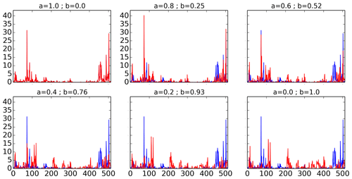
Let us first discuss intuitively the influence of the parameters a and b. Figure 1 displays the fields ϵ_λ (in red) and X_λ (in blue) for a realization of X_λ and Y_λ with α_X=1.8, $C_{\mathrm{1},X}=\mathrm{0.3}$, α_Y=0.8 and $C_{\mathrm{1},Y}=\mathrm{0.3}$ (Eq. 5 is used). Values of a ranging from 1 to 0 are shown. b was tuned to ensure the same C₁ is retrieved on all the fields. For a=1 and b=0 (upper left), the two fields are obviously equal and hence superposed. The opposite case is a=0 and b=1 (lower right), for which ϵ_λ is simply equal to Y_λ, and hence fully independent of X_λ. In the intermediate cases, the progressive decorrelation between the two fields is visible with decreasing values of a. In that sense the parameters a and b characterize the level of correlation between the two fields.

Figure 1 ϵ_λ (in red) and X_λ (in blue) for a realization of X_λ and Y_λ with α_X=1.8, $C_{\mathrm{1},X}=\mathrm{0.3}$, α_Y=0.8 and $C_{\mathrm{1},Y}=\mathrm{0.3}$. Definition of Eq. (5) is used. Various values of a are shown; b is tuned to ensure the same C₁ is retrieved on all the fields.

3.2 Theoretical expectations

In order to evaluate the expected multifractal behaviour of ϵ_λ, its statistical moments of order q are computed to evaluate K_ϵ(q). Given that X_λ and Y_λ are independent, it yields

$$\begin{array}{ll}{\displaystyle }\langle {\mathit{ϵ}}_{\mathit{\lambda }}^q\rangle ={\mathit{\lambda }}^{K_{\mathit{ϵ}}\left(q\right)}& {\displaystyle }={\displaystyle \frac{〈X_{\mathit{\lambda }}^{qa}〉〈Y_{\mathit{\lambda }}^{qb}〉}{{〈X_{\mathit{\lambda }}^a〉}^q{〈Y_{\mathit{\lambda }}^b〉}^q}}\\ \text{(6)}& {\displaystyle }& {\displaystyle }={\mathit{\lambda }}^{K_X\left(qa\right)-q{K}_X\left(a\right)+K_Y\left(qb\right)-q{K}_Y\left(b\right)},\end{array}$$

which means we have

$$\begin{array}{ll}{\displaystyle }{K}_{\mathit{ϵ}}\left(q\right)& {\displaystyle }=a^{{\mathit{\alpha }}_X}{K}_X\left(q\right)+b^{{\mathit{\alpha }}_Y}{K}_Y\left(q\right)\\ {\displaystyle }& {\displaystyle }=a^{{\mathit{\alpha }}_X}{\displaystyle \frac{C_{\mathrm{1},X}}{{\mathit{\alpha }}_X-\mathrm{1}}}(q^{{\mathit{\alpha }}_X}-q)+b^{{\mathit{\alpha }}_Y}{\displaystyle \frac{C_{\mathrm{1},Y}}{{\mathit{\alpha }}_Y-\mathrm{1}}}(q^{{\mathit{\alpha }}_Y}-q)\\ \text{(7)}& {\displaystyle }& {\displaystyle }\approx {\displaystyle \frac{C_{\mathrm{1},\mathit{ϵ}}}{{\mathit{\alpha }}_{\mathit{ϵ}}-\mathrm{1}}}(q^{{\mathit{\alpha }}_{\mathit{ϵ}}}-q).\end{array}$$

The exact computation of K_ϵ(q) is written in the second line of Eq. (7). The third line is not exact and corresponds the form K_ϵ(q) would have if ϵ_λ was actually a UM. This is not true in the general case. In order to assess pseudo-UM parameters C_1,ϵ and α_ϵ, we suggest to use the properties of Eq. (3) and equalize the first and second derivatives of the two last lines of Eq. (7) for q=1. This yields

$$\begin{array}{ll}{\displaystyle }{C}_{\mathrm{1},\mathit{ϵ}}& {\displaystyle }=C_{\mathrm{1},X}{a}^{{\mathit{\alpha }}_X}+C_{\mathrm{1},Y}{b}^{{\mathit{\alpha }}_Y},\\ \text{(8)}& {\displaystyle }{\mathit{\alpha }}_{\mathit{ϵ}}& {\displaystyle }={\displaystyle \frac{C_{\mathrm{1},X}{a}^{{\mathit{\alpha }}_X}{\mathit{\alpha }}_X+C_{\mathrm{1},Y}{b}^{{\mathit{\alpha }}_Y}{\mathit{\alpha }}_Y}{C_{\mathrm{1},X}{a}^{{\mathit{\alpha }}_X}+C_{\mathrm{1},Y}{b}^{{\mathit{\alpha }}_Y}}}.\end{array}$$

It should be noted that in the specific case of α_X=α_Y, α_ϵ is also equal to this value and ϵ_λ is actually an exact UM field.

Figure 2 displays the scaling moment functions of the previously discussed fields for various sets of parameters. Similar results are found for other sets of UM parameters and combinations of a and b exponents. In Fig. 2a, the same α is used for both X_λ and Y_λ, and the expected exact UM behaviour is correctly retrieved. When α_X≠α_Y, ϵ_λ is not exactly a UM. As it is illustrated in Fig. 2b and c, the smaller the differences, the better the UM approximation for ϵ_λ. In the extreme case when α_Y=0 (Fig. 2c), the approximation remains valid only for q ranging from ∼0.6 to 1.6. This range is much wider when the α values are closer. It should be noted that for great moments, some discrepancies are visible, with the exact value of K_ϵ(q) always being greater than its UM approximation. This could wrongly be interpreted suggesting that a multifractal phase transition associated with the divergence of moments is occurring, whereas it is merely an illustration of the limits of validity of the approximation of ϵ_λ as a UM field. Indeed, the values of q_D are much greater than the moment for which the discrepancies start to be visible. In the cases of Fig. 2, we have q_D=5.96 for panel (a), q_D=4.58 for panel (b) and q_D=119 for panel (c), for which the approximation as a UM field is less valid. These values are obtained by looking for the solution >1 to the equation $K\left(q_D\right)=(q_D-\mathrm{1})D$ using the pseudo-UM parameters of ϵ_λ (D is the dimension of the embedding space and is equal to 1 for time series). When confronted with such behaviour, keeping in mind this sort of interpretation could be interesting.

Figure 2 Illustration of the scaling moment functions K(q) of X_λ, Y_λ and ϵ_λ, along with the UM approximation for ϵ_λ (fitted around q=1). Three possible sets of parameters are displayed.

3.3 Techniques for retrieving parameters

In this sub-section an empirical technique to estimate the UM parameters of Y_λ and the exponents a and b from a joint multifractal analysis of X_λ and ϵ_λ is presented. The following steps should be implemented:

• Step 1: performing a UM analysis of each field X_λ and ϵ_λ independently. This enables the quality of the scaling behaviour to be confirmed and α_X, C_1,X, α_ϵ and C_1,ϵ to be estimated. Without any loss of generality, we can assume that $C_{\mathrm{1},Y}=C_{\mathrm{1},X}$. Indeed C_1,Y is a rather arbitrary quantity that can be changed while the one that actually matters is $C_{\mathrm{1},Y}{b}^{{\mathit{\alpha }}_Y}$.

• Step 2: estimating a. This is actually the trickiest portion of the process and requires a joint multifractal analysis. More precisely Eq. (4) is implemented with X_λ and ϵ_λ. In that case, it turns out that the ratio does not depend any more on Y_λ but only on X_λ. One obtains

  $$\begin{array}{ll}{\displaystyle }r(q,h)& {\displaystyle }=K_X(ha+q)-K\left(ha\right)-K\left(q\right)\\ \text{(9)}& {\displaystyle }& {\displaystyle }={\displaystyle \frac{C_{\mathrm{1},X}}{{\mathit{\alpha }}_X-\mathrm{1}}}\left(\right(ha+q{)}^{{\mathit{\alpha }}_X}-(ha{)}^{{\mathit{\alpha }}_X}-(q{)}^{{\mathit{\alpha }}_X}).\end{array}$$

  Hence, for a given value of h and q, r(q,h) is an increasing function of a. This property is used to compute an estimate of a. The simplest approach is to set h and q, compute an empirical value of r_emp(q,h), and find the a that yields this value. When implementing this technique, one should keep in mind that empirical fields are subject to multifractal phase transitions affecting their scaling behaviour. This means that ha+q, ha and q should remain within the range of values for which the estimations of the scaling moment functions remain reliable, i.e. smaller that the corresponding q_s and q_D.

• Step 3: estimating α_Y. Using Eq. (8), one can easily obtain the following (noting that ${\mathit{\alpha }}_{\mathit{ϵ}}{C}_{\mathrm{1},\mathit{ϵ}}=C_{\mathrm{1},X}{a}^{{\mathit{\alpha }}_X}{\mathit{\alpha }}_X+C_{\mathrm{1},Y}{b}^{{\mathit{\alpha }}_Y}{\mathit{\alpha }}_Y$, and that the term $C_{\mathrm{1},Y}{b}^{{\mathit{\alpha }}_Y}$ is simply equal to $C_{\mathrm{1},\mathit{ϵ}}-C_{\mathrm{1},X}{a}^{{\mathit{\alpha }}_X}$, which enables the non-linear part of the equation to be removed):

  $$\begin{array}{}\text{(10)}& {\mathit{\alpha }}_Y={\displaystyle \frac{\frac{C_{\mathrm{1},\mathit{ϵ}}}{C_{\mathrm{1},X}}{\mathit{\alpha }}_{\mathit{ϵ}}-a^{{\mathit{\alpha }}_X}{\mathit{\alpha }}_X}{\frac{C_{\mathrm{1},\mathit{ϵ}}}{C_{\mathrm{1},X}}-a^{{\mathit{\alpha }}_X}}}.\end{array}$$

• Step 4: computing b. Once α_Y is known, Eq. (8) (top) can be used to estimate b as follows (noting that $C_{\mathrm{1},Y}{b}^{{\mathit{\alpha }}_Y}=C_{\mathrm{1},\mathit{ϵ}}-C_{\mathrm{1},X}{a}^{{\mathit{\alpha }}_X}$ and that we have $C_{\mathrm{1},Y}=C_{\mathrm{1},X}$):

  $$\begin{array}{}\text{(11)}& b={\left({\displaystyle \frac{C_{\mathrm{1},\mathit{ϵ}}}{C_{\mathrm{1},X}}}-a^{{\mathit{\alpha }}_X}\right)}^{\mathrm{1}/{\mathit{\alpha }}_Y}.\end{array}$$

3.4 Implementation on numerical simulations (discrete UM)

The approach presented above is tested on numerical simulations obtained with discrete in-scale cascades. It consists of iteratively repeating a cascade step with a non-infinitesimal scale ratio in which a “parent” structure is divided into “daughter” structures whose affected value is the one of the “parent” structure multiplied by a random factor, ensuring that Eqs. (1) and (2) remain valid. Such a simple field generation process is sufficient for the purposes of this paper. The recent introduction of multifractal operators and vectors paves the way for physically based, continuous (in-scale) multivariate analysis of multifractal fields or measures (Schertzer and Tchiguirinskaia, 2015, 2020).

A set of 10 000 realizations of 512 long 1D discrete cascades is used, and analyses are carried out on ensemble averages.

Before starting, let us clarify the objective of this section. X_λ and Y_λ are first simulated and then ϵ_λ is built with some values of a and b. The purpose is to retrieve the values of a, b and α_Y by simply analysing X_λ and ϵ_λ, which are assumed to be known.

The parameters used for these simulations are α_X=1.8, $C_{\mathrm{1},X}=\mathrm{0.3}$, α_Y=0.8, $C_{\mathrm{1},Y}=\mathrm{0.3}$, a=0.6 and b=0.2. As a consequence we expect to find α_ϵ=1.39 and $C_{\mathrm{1},\mathit{ϵ}}=\mathrm{0.20}$. Other sets of parameters have been tested and yield similar results.

Results of this analysis are displayed in Fig. 3. As expected, the scaling behaviour observed on both X_λ and ϵ_λ is excellent. TM analysis, i.e. Eq. (1) in a log–log plot, for ϵ_λ is shown in Fig. 3a and all the coefficients of determination of the straight lines used to compute K(q) are greater than 0.99. With regard to the estimates of UM parameters retrieved via the DTM technique, for X_λ they are equal to 1.79 and 0.27 for α and C₁ respectively, which is close to the values input in the simulations. The small discrepancy in C₁ has already been noted with such discrete simulations. The respective estimates for ϵ_λ are 1.35 and 0.18, which are in agreement with the theoretical expectations. These small differences are visible in Fig. 3b, which displays the empirical and theoretical fitting of K(q). For X_λ, it can be noted that the empirical estimate of K(q) is smaller that its theoretical value (using UM estimates retrieved from the DTM analysis) for q greater than ∼1.7. This is consistent with a behaviour affected by the multifractal phase transition associated with sampling limitations (q_s=1.95 for the input UM parameters). It can be noted that for ϵ_λ we have a greater q_s equal to 1.95, while it is even greater for Y_λ(=4.5). The values of q_D are greater in all cases, meaning that the multifractal phase transition associated with divergence of moment will not bias our analysis.

In order to estimate a (step 2 of the process described in the previous sub-section), we consider the two moments $q=h=\mathrm{0.7}$. Note that with these values we have $ha+q=\mathrm{1.12}$, which is much smaller than the minimum q_s for the chosen values of UM parameters. This means that the estimates should not be affected by expected biases associated with multifractal phase transitions. Figure 3c shows the output of the joint multifractal (Eq. 4 in log–log plot). It appears that the scaling is excellent and the slope gives an estimate of r(0.7,0.7). It is then used to estimate a by adjusting the value of a so that r(0.7,0.7)(a) equals the computed empirical value (Fig. 3d). This yields a=0.59. Finally (Eqs. 10 and 11) we obtain an estimate of b equal to 0.20 and an estimate of α_Y equal to 0.77. These values are very close to those input in the simulations. In summary, there is a very good agreement between theoretical expectations and numerical simulations, which confirms the validity of the framework presented in this section.

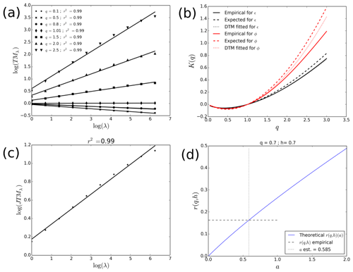
Figure 3 Results of numerical analysis with α_X=1.8, $C_{\mathrm{1},X}=\mathrm{0.3}$, α_Y=0.8, $C_{\mathrm{1},Y}=\mathrm{0.3}$, a=0.6 and b=0.2 as input parameters. (a) TM analysis i.e. Eq. (1) in log–log plot, for ϵ_λ. (b) Scaling moment functions K(q) for ϵ_λ and X_λ. (c) Joint multifractal analysis (Eq. 4 in log–log plot) for $q=h=\mathrm{0.7}$. (d) Illustration of the estimation of a with the values r(0.7,0.7) computed in  (c).

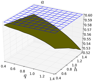
Finally, let us discuss the uncertainties in the estimates of a. Fig. 4 displays the estimates of a on the simulated fields (see Fig. 3) as a function of the moment orders q and h used in the joint multifractal analysis. It appears that as long as the studied moments remain within the range of reliability of the multifractal analysis (i.e. $ha+q<q_s$ as previously discussed), the estimates are rather stable. For greater values, there is an underestimation of a.

Figure 4 Estimate of a on the simulated fields (see Fig. 3) as a function of the moment orders q and h used in the joint multifractal analysis. The blue grid at the constant value of 0.6 corresponds to the value of a inputted in the simulations.

4 Toward an indicator of correlation

Let us consider two fields ϵ_λ and ϕ_λ. It is assumed that they both exhibit UM properties, with known UM parameters. The purpose of this section is to present a framework to study the correlations across scales between the two fields. This relies on the joint multifractal analysis presented in Sect. 2.1, with the suggestion of a simplified indicator. It furthermore opens the path to numerical simulations of one field from the other.

More precisely, the consequences of describing each field as a multiplicative power law combination of the other and an independent one will be explored. The notations are

$$\begin{array}{ll}{\displaystyle }{\mathit{ϵ}}_{\mathit{\lambda }}& {\displaystyle }={\displaystyle \frac{{\mathit{\varphi }}_{\mathit{\lambda }}^a{Y}_{\mathit{\lambda }}^b}{〈{\mathit{\varphi }}_{\mathit{\lambda }}^a{Y}_{\mathit{\lambda }}^b〉}},\\ \text{(12)}& {\displaystyle }{\mathit{\varphi }}_{\mathit{\lambda }}& {\displaystyle }={\displaystyle \frac{{\mathit{ϵ}}_{\mathit{\lambda }}^{a^{\prime }}{Z}_{\mathit{\lambda }}^{b^{\prime }}}{〈{\mathit{ϵ}}_{\mathit{\lambda }}^{a^{\prime }}{Z}_{\mathit{\lambda }}^{b^{\prime }}〉}},\end{array}$$

where a, b, a^′ and b^′ characterize the level of correlation between the two fields, while Y_λ and Z_λ are independent random UM fields. As shown in the previous section, without any loss of generality it can be assumed that $C_{\mathrm{1},Y}=C_{\mathrm{1},\mathit{\varphi }}$ and $C_{\mathrm{1},Z}=C_{\mathrm{1},\mathit{ϵ}}$. This enables the following calculations to be simplified.

4.1 Limitations of this symmetric framework

If both lines of Eq. (12) were to be correct, then the joint multifractal correlation of ϵ_λ and ϕ_λ could be computed in two equivalent ways:

$$\begin{array}{ll}{\displaystyle \frac{〈{\mathit{ϵ}}_{\mathit{\lambda }}^q{\mathit{\varphi }}_{\mathit{\lambda }}^h〉}{〈{\mathit{ϵ}}_{\mathit{\lambda }}^q〉〈{\mathit{\varphi }}_{\mathit{\lambda }}^h〉}}& {\displaystyle }={\displaystyle \frac{〈{\mathit{\varphi }}_{\mathit{\lambda }}^{aq+h}{Y}_{\mathit{\lambda }}^{bq}〉}{〈{\mathit{\varphi }}_{\mathit{\lambda }}^{ah}〉〈Y_{\mathit{\lambda }}^{bq}〉〈{\mathit{\varphi }}_{\mathit{\lambda }}^q〉}}={\displaystyle \frac{〈{\mathit{\varphi }}_{\mathit{\lambda }}^{aq+h}〉}{〈{\mathit{\varphi }}_{\mathit{\lambda }}^{aq}〉〈{\mathit{\varphi }}_{\mathit{\lambda }}^h〉}}\\ {\displaystyle }& {\displaystyle }={\mathit{\lambda }}^{r_{\mathit{ϵ}\mathit{\varphi }}(q,h)}={\mathit{\lambda }}^{\frac{C_{\mathrm{1},\mathit{\varphi }}}{{\mathit{\alpha }}_{\mathit{\varphi }}-\mathrm{1}}\left[\right(aq+h{)}^{{\mathit{\alpha }}_{\mathit{\varphi }}}-(aq{)}^{{\mathit{\alpha }}_{\mathit{\varphi }}}-(h{)}^{{\mathit{\alpha }}_{\mathit{\varphi }}}]},\\ {\displaystyle \frac{〈{\mathit{ϵ}}_{\mathit{\lambda }}^q{\mathit{\varphi }}_{\mathit{\lambda }}^h〉}{〈{\mathit{ϵ}}_{\mathit{\lambda }}^q〉〈{\mathit{\varphi }}_{\mathit{\lambda }}^h〉}}& {\displaystyle }={\displaystyle \frac{〈{\mathit{ϵ}}_{\mathit{\lambda }}^{q+a^{\prime }h}{Z}_{\mathit{\lambda }}^{h{b}^{\prime }}〉}{〈{\mathit{ϵ}}_{\mathit{\lambda }}^q〉〈{\mathit{ϵ}}_{\mathit{\lambda }}^{a^{\prime }h}〉〈Z_{\mathit{\lambda }}^{h{b}^{\prime }}〉}}={\displaystyle \frac{〈{\mathit{ϵ}}_{\mathit{\lambda }}^{q+a^{\prime }h}〉}{〈{\mathit{ϵ}}_{\mathit{\lambda }}^q〉〈{\mathit{ϵ}}_{\mathit{\lambda }}^{a^{\prime }h}〉}}\\ \text{(13)}& {\displaystyle }& {\displaystyle }={\mathit{\lambda }}^{r_{\mathit{\varphi }\mathit{ϵ}}(q,h)}={\mathit{\lambda }}^{\frac{C_{\mathrm{1},\mathit{ϵ}}}{{\mathit{\alpha }}_{\mathit{ϵ}}-\mathrm{1}}\left[\right(q+a^{\prime }h{)}^{{\mathit{\alpha }}_{\mathit{ϵ}}}-(q{)}^{{\mathit{\alpha }}_{\mathit{ϵ}}}-(a^{\prime }h{)}^{{\mathit{\alpha }}_{\mathit{ϵ}}}]},\end{array}$$

leading to

$$\begin{array}{ll}{\displaystyle }\forall h,q& {\displaystyle \frac{C_{\mathrm{1},\mathit{\varphi }}}{{\mathit{\alpha }}_{\mathit{\varphi }}-\mathrm{1}}}\left[\right(qa+h{)}^{{\mathit{\alpha }}_{\mathit{\varphi }}}-(qa{)}^{{\mathit{\alpha }}_{\mathit{\varphi }}}-(h{)}^{{\mathit{\alpha }}_{\mathit{\varphi }}}]\\ \text{(14)}& {\displaystyle }& {\displaystyle }={\displaystyle \frac{C_{\mathrm{1},\mathit{ϵ}}}{{\mathit{\alpha }}_{\mathit{ϵ}}-\mathrm{1}}}\left[(q+a^{\prime }h{)}^{{\mathit{\alpha }}_{\mathit{ϵ}}}-(q{)}^{{\mathit{\alpha }}_{\mathit{ϵ}}}-(a^{\prime }h{)}^{{\mathit{\alpha }}_{\mathit{ϵ}}}\right].\end{array}$$

In the general case, Eq. (14) is not valid for any q and h. To better understand this, let us consider a given level of correlation by setting the parameters a and b. The goal is to compute a^′ and b^′ from the available parameters. The left-hand side of Eq. (14) is known, and after setting given values of q and h it is possible to implement the same process as in Sect. 3.3 to determine a^′, b^′ and α_Z. Figure 5 displays the outcome of this analysis, according to the values of h and q used, for a=0.2 in the case α_ϵ=0.8, $C_{\mathrm{1},\mathit{ϵ}}=\mathrm{0.4}$, α_ϕ=0.8, $C_{\mathrm{1},\mathit{\varphi }}=\mathrm{0.2}$ (meaning that b=0.30 and α_Y=0.68). As can be seen, the estimates of a^′ exhibit a dependency on q and h. The dependency is stronger on q than on h and estimates remain rather stable as long as q<0.8. Both sides of Eq. (14) are plotted in Fig. 6 for this set of UM parameters with a=0.2 and estimates of $a^{\prime }=\mathrm{0.19}$ obtained with $h=q=\mathrm{0.7}$. Expected differences are visible for the larger values of h and q. It should be mentioned that these results are presented for a bad case with strong differences between α_ϵ and α_ϕ. They are actually much smaller if both values are closer to 2. For the specific case, ${\mathit{\alpha }}_{\mathit{ϵ}}={\mathit{\alpha }}_{\mathit{\varphi }}=\mathrm{2}$, Eq. (14) becomes

$$\begin{array}{}\text{(15)}& \forall h,q{C}_{\mathrm{1},\mathit{\varphi }}ahq=C_{\mathrm{1},\mathit{ϵ}}{a}^{\prime }hq,\end{array}$$

meaning that once hq has been removed, a^′ is deterministically obtained once a is set and $r_{\mathit{ϵ}\mathit{\varphi }}(q,h)=r_{\mathit{ϵ}\mathit{\varphi }}(q,h)=C_{\mathrm{1},\mathit{\varphi }}ahq$ is linear with regard to h and q.

Figure 5 Estimates of a^′ as a function of h and q using Eq. (14) and the process described in Sect. 3.3. Computations are carried out with α_ϵ=0.8, $C_{\mathrm{1},\mathit{ϵ}}=\mathrm{0.4}$, α_ϕ=0.8, $C_{\mathrm{1},\mathit{\varphi }}=\mathrm{0.2}$ and a=0.2. The blue horizontal grid corresponds to the value obtained with Eq. (17).

Figure 6 Both sides of Eq. (14) for α_ϵ=0.8, $C_{\mathrm{1},\mathit{ϵ}}=\mathrm{0.4}$, α_ϕ=0.8 and $C_{\mathrm{1},\mathit{\varphi }}=\mathrm{0.2}$ in the case a=0.2 and $a^{\prime }=\mathrm{0.19}$. r_ϵϕ(q,h) is in red and corresponds to the left-hand side of Eq. (14) while r_ϕϵ(q,h) is the right-hand side and is in blue. Two views of the same figure are provided to improve visualization.

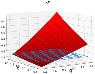
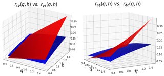
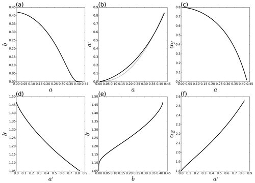
Figure 7 illustrates the relation between the parameters retrieved by setting different values of a in the same case α_ϵ=0.8, $C_{\mathrm{1},\mathit{ϵ}}=\mathrm{0.4}$, α_ϕ=0.8, $C_{\mathrm{1},\mathit{\varphi }}=\mathrm{0.2}$. First it should be mentioned that for a given set of UM parameters, not all values of a are possible. Indeed the inequality $\mathrm{0}\le {\mathit{\alpha }}_Y\le \mathrm{2}$ must be respected, leading to $a\le min\left[\right(\frac{C_{\mathrm{1},\mathit{ϵ}}{\mathit{\alpha }}_{\mathit{ϵ}}}{C_{\mathrm{1},\mathit{\varphi }}{\mathit{\alpha }}_{\mathit{\varphi }}}{)}^{\mathrm{1}/{\mathit{\alpha }}_{\mathit{\varphi }}},\left(\frac{C_{\mathrm{1},\mathit{ϵ}}(\mathrm{2}-{\mathit{\alpha }}_{\mathit{ϵ}})}{C_{\mathrm{1},\mathit{\varphi }}(\mathrm{2}-{\mathit{\alpha }}_{\mathit{\varphi }})}{)}^{\mathrm{1}/{\mathit{\alpha }}_{\mathit{\varphi }}}\right]$. In this case we must have a≤0.43. We retrieved the expected behaviour and are able to quantify it: b decreases with increasing a (Fig. 7a), a^′ increases with increasing a (Fig. 7b), α_Y decreases with increasing a (Fig. 7c), and similar behaviour is found in terms of dependency in a^′ for the symmetric case.

Figure 7 Illustration of the relations between the various parameters characterizing the correlation across scales between two UM fields in the case α_ϵ=0.8, $C_{\mathrm{1},\mathit{ϵ}}=\mathrm{0.4}$, α_ϕ=0.8 and $C_{\mathrm{1},\mathit{\varphi }}=\mathrm{0.2}$. The dash line in (b) corresponds to the relation obtained by implementing Eq. (17).

4.2 A simplified indicator

In Sect. 4.1, limitations of this fully symmetric framework are highlighted. However, it is possible to suggest a rather intuitive indicator enabling most of the information obtained from the joint multifractal correlation analysis (i.e. the computation of r(q,h)) to be extracted. This corresponds to the portion of intermittency C₁ of one field explained by the other:

$$\begin{array}{ll}{\displaystyle }{\text{IC}}_{\mathit{ϵ}\mathit{\varphi }}& {\displaystyle }={\displaystyle \frac{C_{\mathrm{1},\mathit{\varphi }}{a}^{{\mathit{\alpha }}_{\mathit{\varphi }}}}{C_{\mathrm{1},\mathit{ϵ}}}},\\ \text{(16)}& {\displaystyle }{\text{IC}}_{\mathit{\varphi }\mathit{ϵ}}& {\displaystyle }={\displaystyle \frac{C_{\mathrm{1},\mathit{ϵ}}{a}^{\prime {\mathit{\alpha }}_{\mathit{ϵ}}}}{C_{\mathrm{1},\mathit{\varphi }}}}.\end{array}$$

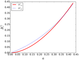
Both “indicators of correlation” (ICs) are displayed in Fig. 8 for the data corresponding to Fig. 7. Both curves are close, and this symmetric behaviour is what is wanted for such an indicator of correlation. Again, much closer curves are obtained with greater values of α and identical curves are retrieved when the α of ϵ and ϕ are both equal to 2. Forcing IC_ϵϕ=IC_ϕϵ can actually be a way to find an estimate of a^′ once a is known without having to implement the process described above. It yields

$$\begin{array}{}\text{(17)}& {\displaystyle }{a}^{\prime }={\left({\displaystyle \frac{C_{\mathrm{1},\mathit{\varphi }}}{C_{\mathrm{1},\mathit{ϵ}}}}\right)}^{\mathrm{2}/{\mathit{\alpha }}_{\mathit{ϵ}}}{a}^{{\mathit{\alpha }}_{\mathit{\varphi }}/{\mathit{\alpha }}_{\mathit{ϵ}}}.\end{array}$$

Equation (17) is actually plotted in a dashed line in Fig. 7b and provides very good estimates. Hence this IC appears to be a good candidate for characterizing in a simple way the correlations across scales between two fields. One should keep in mind that it is mainly relevant in the case where the studied fields do not exhibit values of α that are too small (typically <0.8).

Figure 8 Plot of IC_ϵϕ and IC_ϕϵ as a function of a (Eq. 17) for the same data that is presented in Fig. 7.

5 Implementation on rainfall data

5.1 Presentation of the data

The rainfall data used in this paper were collected by a OTT Parsivel² disdrometer (Battaglia et al., 2010; OTT, 2014) located on the roof of the Carnot building of the Ecole des Ponts ParisTech campus near Paris between 15 January 2018 and 9 December 2018. It is part of the TARANIS observatory of the Fresnel Platform of École des Ponts ParisTech (https://hmco.enpc.fr/portfolio-archive/fresnel-platform/, last access: 12 March 2020). Data are collected with 30 s time steps. Data will only be briefly presented in this paper and interested readers are referred to Gires et al. (2018b), who discusses available database in detail along with some data samples for a similar measurement campaign.

In this paper four quantities are studied:

• R, the rain rate (mm h⁻¹);

• LWC, the liquid water content (g m⁻³);

• N_t, the total drop concentration (m⁻³);

• D_m, the mass weight diameter (mm).

N_t and D_m are used to characterize the drop size distribution (DSD, N(D), ${\mathrm{m}}^{-\mathrm{3}}{\mathrm{mm}}^{-\mathrm{1}}$) of the rainfall. N(D)dD is the number of drops per unit volume (in m⁻³) with an equivolumic diameter between D and D+dD (in mm). DSDs are commonly written in the form N(D)=N_tf(D_m), with D_m being an indicator of the shape of the DSD and N_t an indicator of the total intensity. They can be computed from the DSD as follows (Leinonen et al., 2012; Jaffrain and Berne, 2012):

$$\begin{array}{}\text{(18)}& {\displaystyle }& {\displaystyle }{N}_{\mathrm{t}}=\underset{D_{min}}{\overset{D_{max}}{\int }}N\left(D\right)\mathrm{d}D,\text{(19)}& {\displaystyle }& {\displaystyle }{D}_{\mathrm{m}}={\displaystyle \frac{{\int }_{D_{min}}^{D_{max}}N\left(D\right)D^{\mathrm{4}}\mathrm{d}D}{{\int }_{D_{min}}^{D_{max}}N\left(D\right)D^{\mathrm{3}}\mathrm{d}D}}.\end{array}$$

It should be noted that the disdrometer provides data binned per class of equivolumic diameter and fall velocity, from which a discrete DSD is computed and then used to evaluate the integrals of Eqs. (18) and (19) (see Gires et al., 2018b, for more details).

Multifractal analyses are carried out on ensemble analyses, i.e. on average over various samples. Once rainfall events (an event is defined as a rainy period during which more than 1 mm is collected and that is separated by more than 15 min of dry conditions before and after) have been selected within the longer time series, a process similar to in Gires et al. (2016) and Gires et al. (2018a) is implemented to extract the various samples of data: “for each event (i) a sample size is chosen (a power of two, if possible); (ii) the maximum number of samples for this event is computed; (iii) the portion of the event of length equal to the sample size multiplied by the number of samples found in (ii) with the greatest cumulative depth is extracted; (iv) the extracted series is cut into various samples.” Since D_m is not defined when there is no rain, only samples with no zeros are used.

Dyadic sample sizes are simpler to use for multifractal analysis, which results in some data not being used. With the process described above, 63, 52, 38 and 22 % of the data is actually not used for sample sizes of 32, 64, 128 and 256 respectively. A size of 32 time steps, corresponding to 16 min, is used, to maximize the amount of data used while keeping an acceptable length for the studied time series. An example of a sample for the four studied quantities during a rainfall event that occurred on 15 January 2018 is shown in Fig. 9. A total of 491 such samples are used in the analysis.

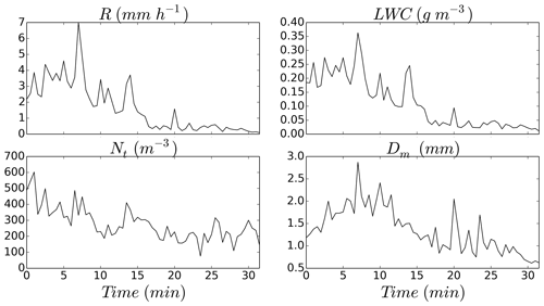
Figure 9 Illustration of the four studied rainfall quantities corresponding to a 32 min sample (i.e. 64 time steps) that occurred on 15 January 2018.

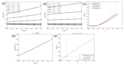
Figure 10 Results of joint multifractal analysis for ϵ_λ being the fluctuations of N_t and ϕ_λ being the fluctuations of R. (a) TM analysis, i.e. Eq. (1) in log–log plot, for ϵ_λ. (b) Same as in (a) for ϕ_λ. (c) Scaling moment functions K(q) for ϵ_λ and ϕ_λ. (d) Joint multifractal analysis (Eq. 4 in log–log) for $q=h=\mathrm{0.7}$. (e) Illustration of the estimation of a with the values r(0.7,0.7) computed in (d).

5.2 Joint analysis and discussion

Let us first discuss the results of the joint multifractal analysis carried out between N_t and R. The purpose is to check if the scale-invariant analysis of correlations is relevant for these fields and then to quantify their correlations in this framework (i.e. write the fields as in Eq. 12 (top) and estimate a, b and α_Y from the two fields only).

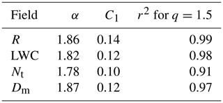
The main curves are shown in Fig. 10, with ϵ_λ being the fluctuations of N_t and ϕ_λ being the fluctuations of R. The analysis directly on the field showed that they were non-conservative, meaning that the TM and DTM analysis would be biased. Hence multifractal analysis was carried out on an approximation of the underlying conservative fields consisting of their fluctuations (Lavallée et al., 1993). Numerical values of the various parameters of the analysis are in Tables 1 and 2. R exhibits a very good scaling behaviour on the whole range of scales taken into account, as shown by the TM analysis where the coefficients of correlation r² of the linear regressions for q around 1 are all greater than 0.98 (Fig. 10b). Similar scaling behaviour was found on a previous campaign with the same devices (Gires et al., 2016). The scaling for N_t is worse, with r² values only slightly greater than 0.9, but it remains acceptable (Fig. 10a). We find α_R=1.86 and $C_{\mathrm{1},R}=\mathrm{0.14}$ and ${\mathit{\alpha }}_{N_{\mathrm{t}}}=\mathrm{1.78}$ and $C_{\mathrm{1},N_{\mathrm{t}}}=\mathrm{0.10}$. The values of UM parameters observed mean that we are in the domain of highest relevance of the framework developed in the previous section. For R, and to a lesser extent N_t, there is a clear departure of the fitted K(q) from the empirical K(q), with much greater values for the fitted curve. Furthermore the empirical K(q) values exhibit a linear behaviour for q greater than approximately 1.5 (Fig. 10c). Such behaviour is consistent with the expected one when a multifractal phase transition associated with sampling limitations occurs.

Table 1 UM parameters for the studied fields.

The joint multifractal analysis (Eq. 4 in log–log) for $q=h=\mathrm{0.7}$ of the two studied fields is displayed in Fig. 10d. The scaling is good, with a value of r²=0.97 for the linear fit. It enables the exponents a and b to be estimated at 0.33 and 0.75 respectively (Fig. 10e). The corresponding IC is equal to 0.18. In addition to quantifying the level of correlations between the two fields, it suggests how to simulate one from the other. More precisely, once a time series of fluctuations of R is available, it is possible to simulate a realistic corresponding time series of fluctuations of N_t, by raising to the power a=0.33 the R series and multiplying it with an independent random field Y with α=1.76 and C₁=0.14 raised to the power b=0.75, and renormalizing the ensemble. Formally it suggests the fluctuations of N_t can be written as

$${\displaystyle \frac{R_{\text{fluctuations}}^{\mathrm{0.33}}{Y}^{\mathrm{0.75}}}{〈R_{\text{fluctuations}}^{\mathrm{0.33}}{Y}^{\mathrm{0.75}}〉}}.$$

Such relations open the path for techniques to simulate fluctuations of N_t knowing only the temporal evolution of the rain rate.

Table 2 Numerical output of the joint multifractal analysis of the four studied fields. For each box, using the notations of Eq. (12) ϵ_λ corresponds to the field of the column and ϕ_λ to the row.

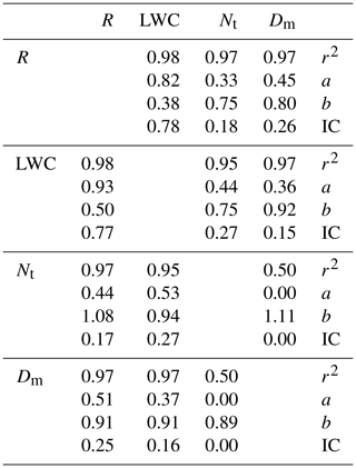
Similar qualitative results are found for the other combinations, and numerical values are reported in Table 1. Both LWC and D_m exhibit a good scaling behaviour and their UM parameters are in Table 1. As expected given the observed values of α, the ICs computed in one way or the other (i.e. inverting the role of ϵ_λ and ϕ_λ) are very similar. Furthermore the values of a^′ found using Eq. (17) (not shown) are very close to those obtained by inverting the role of the two fields. This confirms the relevancy of the framework of Sect. 4 in this case. It appears that the correlation found between R and LWC is much stronger than between R and N_t or D_m. There is no correlation between N_t or D_m which suggests but is not proof of independence (it would be proof for Gaussian variables). Note that the very bad scaling for the joint analysis of these two quantities is partially due to the very small values found for r(q,h) which are basically equal to zero. R exhibits a slightly greater correlation with D_m (IC=0.26) than with N_t (IC=0.18). It is the inverse for LWC with values of IC equal to 0.15 and 0.27 respectively.

6 Conclusions

In this paper, we used the framework of joint multifractal analysis to characterize the correlation across scales between two multifractal fields. We extended the existing framework to universal multifractals and also to analyse the correlations between two fields consisting of renormalized multiplicative power law combinations of two known UM fields. In general, the resulting fields can be well approximated by UM fields. Estimates of the corresponding pseudo-UM parameters can be theoretically computed by focusing on the behaviour for moments close to one. These estimates remain valid for a range of moments between ∼ 0.6 and ∼ 1.6 in the worst case. The closer the two α of the initial fields, the better the approximation. When both α values are equal, the approximation is exact. An analysis technique to estimate the properties of the underlying fields (UM parameters and power law exponents used in the combination) was developed and validated with the help of numerical simulations.

In a second step, this analysis was used to develop an innovative framework to investigate the correlations between two UM fields. It basically consists of looking at the best parameters, enabling one field to be written as a power law multiplicative combination of the other field and a random one. In this context, a good candidate for a simple indicator of the strength of the correlation (called IC) is the proportion of intermittency of a field explained by the other one. In the general case, this framework is not symmetric, which is a limitation. However when the α values are typically greater than ∼0.8, it is approximately symmetric, meaning that it is relevant to extract some information on the correlations between two fields.

Finally this was implemented on rainfall data collected by a disdrometer installed on the roof the Ecole des Ponts ParisTech. More precisely the correlations between R and LWC and DSD features (N_t and D_m) are investigated. First it should be mentioned that the scaling behaviour of both R and LWC is excellent, while that of the DSD features is only good. The α values are rather similar and greater than 1.7, meaning that it is a favourable context in which to use the newly developed approach. It appears that the correlation between R and LWC is as expected very strong, the one between R or LWC and the DSD features is medium, and the one between N_t and D_m is basically null. Besides quantifying these correlations, the developed framework suggests a simple technique to simulate one field from the other. Indeed, it is sufficient to compute a power law multiplicative combination between one field and a random one to obtain the other. The characteristic parameters of the random field as well as the power law exponents of the relation can be obtained through a joint multifractal analysis of the two studied fields.

Further investigations on other fields in various contexts should be carried out to confirm the ability of this framework to both characterize and simulate correlations across scales between two multifractal fields. In future work, this framework should also be extended to more than two fields.