Data assimilation of coherent structures in parametric and gridded spaces: an idealized ocean eddy study

Data assimilation (DA) combines observations and model background to estimate the state of geophysical systems. Coherent structures, such as ocean eddies, are localized geophysical features characterized by a small set of properties: position, amplitude, and shape for instance. When linear and gaussian DA is applied directly to a gridded field without prior structural adjustment, the linear combination of background and observation can distort these properties, particularly when displacement uncertainty dominates. In this work, we explore a DA framework of coherent structures in a reduced parametric space, where the state is defined by a set of parameters describing the structure. Using an idealized one-dimensional ocean eddy, we compare single-step analyses performed both in gridded and parametric spaces. Three tutorial experiments with prescribed parametric uncertainties illustrate this distortion mechanism directly. A fourth experiment, starting from noisy gridded observations, provides a more balanced evaluation using the inverse nonlinear mapping from grid to parameter space. In these idealized experiments, the parametric approach maintains a physically consistent shape after assimilation. The parametric DA requires reliable parameter extraction, and its benefits depend on the number of structures relative to grid resolution.

1 Introduction

Data assimilation (DA) is widely used in geosciences to combine observations with information from a dynamical model (the background) in a statistically optimal way (Carrassi et al., 2018). In its standard formulation, DA aims to estimate the full system state on a spatial grid.

In this study, we do not focus on the full gridded state, but rather on the estimation of specific geophysical structures (GSs), such as ocean eddies or cyclones, viewed as coherent objects characterized by a small set of parameters. When classic, linear-Gaussian DA methods, such as optimal interpolation or the Kalman filter, are applied directly to a gridded field without prior structural adjustment, the presence of a coherent structure can cause the linear combination of background and observation to distort the reconstructed structure: spatially displaced or differently-shaped realizations are averaged rather than reconciled, which smears the structure whenever displacement or shape, rather than amplitude, uncertainty dominates (Chen and Snyder, 2007; Feyeux et al., 2018).

Several strategies have been proposed to introduce structural information explicitly into the assimilation problem, spanning a spectrum from field-based to more object-oriented representations. A first family augments the state vector with structure parameters directly: Chen and Snyder (2007) added vortex position to the ensemble Kalman filter (EnKF) state, allowing the filter to separate displacement from amplitude errors. This was extended to tropical cyclones by including position, translation speed, and axisymmetric wind structure (Wu et al., 2010), and further to operationally relevant track, wind-radius, and intensity parameters (Kunii, 2015). These approaches define state variables that are directly interpretable as object properties, though they remain tied to a predefined parametric model, in a spirit close to the parametric representation adopted here. A second family instead treats structural errors through geometric transformations or alternative measures of distance in the field representation. Alignment and morphing approaches modify the field geometry to reconcile displaced or differently shaped structures (Ravela et al., 2007; Beezley and Mandel, 2008; Zhen et al., 2025), while displacement data assimilation explicitly estimates the displacement field required for such alignment while enforcing area preservation (Rosenthal et al., 2017). Alternatively, optimal-transport-based approaches modify the metric used to compare background and observations, using the Wasserstein distance to better account for positional errors of coherent structures (Feyeux et al., 2018). A third family operates on adaptive or moving computational meshes that track coherent structures rather than resolving the full domain at uniform resolution: Aydøğdu et al. (2019) developed ensemble DA for adaptive, non-conservative moving-mesh models, and mesh-node positions have since been included directly within the assimilation state itself (Sampson et al., 2021), though in this case the assimilated geometry reflects the numerical discretization rather than the structure's own properties. Feature-informed and Lagrangian-based approaches extract collective descriptors of coherent structures directly from observations, rather than assimilating raw trajectories or fields (Srivastava et al., 2023; Maclean et al., 2017). Non-Gaussian methods such as particle filters (van Leeuwen, 2010; Poterjoy, 2016) can, in principle, handle the nonlinearity associated with displacement and shape uncertainty; part of the difficulty in relating a gridded and a reduced representation, however, lies not solely in this nonlinearity, but in correctly marginalizing, rather than merely interpolating, uncertainty between the two spaces, a distinction examined further in Sect. 2.1.

Correctly linking uncertainty across representation spaces is itself motivated by a broader principle: Rao-Blackwellization (Casella and Robert, 1996) formalizes the idea of analytically marginalizing a conditionally-linear-Gaussian subset of a state while treating the remaining nonlinear component separately, seeking a representation in which a problem becomes, and remains, Gaussian-tractable. This principle underlies Rao-Blackwellized particle filters (Chen and Liu, 2000), including applications to environmental data assimilation that combine Kalman-type updates with particle-based treatment of low-dimensional non-Gaussian parameters (Šmídl and Hofman, 2011). The parametric transformation explored in this study follow this approach: rather than operating directly on the full gridded field, it seeks a lower-dimensional, physically interpretable representation in which relating background and observation uncertainty is more tractable, provided this relationship is established by propagating the full uncertainty through the mapping between spaces, rather than by a local linear approximation of it.

The goal of this study is to investigate, in a controlled and idealized framework, how the choice of representation space influences the behavior of a standard Gaussian linear DA update when applied to coherent structures with uncertain position and shape. In particular, we compare assimilation performed in the classic gridded space with assimilation performed directly in a reduced parametric space describing the structure.

The idea of working in a low-dimensional parameter space rather than on a full-state vector has a long history in the control and stochastic filtering literature (Jazwinski, 1970). However, in these frameworks, the parameters to be estimated are typically internal coefficients of a dynamical model, rather than geometric descriptors of coherent structures. The present work applies a related principle to an explicitly geometric and physically interpretable representation of a coherent structure, defined here by amplitude, position and radius.

This parametric perspective is also related to reduced-order and subspace approaches, where the system state is represented in a lower-dimensional space, such as empirical orthogonal functions or learned latent variables (Hannachi et al., 2007; Alvera-Azcárate et al., 2025). In contrast to these approaches, which define reduced coordinates in an abstract basis, the present work considers an explicit physically interpretable parameterization of the structure. This allows a direct interpretation of assimilation updates in terms of physically meaningful geometric properties.

We emphasize that this framework does not aim to replace existing Lagrangian, feature-based, or non-Gaussian DA methods, but rather to provide a simplified setting to analyze how standard Gaussian updates behave when applied either in gridded space or in a low-dimensional parameter space representing coherent structures. To the best of our knowledge, this specific comparison of the assimilation behavior between gridded space and an explicitly defined geometric parameter space of a coherent structure has not been analyzed in the literature. In this sense, the study is primarily methodological and diagnostic, focusing on the mechanism of error representation rather than on operational forecasting performance.

In the proposed framework, the state of the system is fully described by the parameters of a single idealized eddy, which allows a direct analysis of how uncertainties in amplitude, position, and radius propagate through the assimilation step in both representations. The computational implications of this lower-dimensional representation are discussed in Sect. 4.4.

We present a set of idealized numerical experiments designed to compare a single analysis step performed in the classic gridded space and in this reduced parametric space. The eddy representation and assimilation methodology are detailed in Sect. 2, the experimental setup in Sect. 3, and the results are presented in Sect. 4. Conclusions and perspectives are discussed in Sect. 5.

2 Methodology

The objective of this paper is to compare two methods of blending two sources of information, a background and an observation, using a basic DA algorithm. We focus exclusively on the analysis step and do not perform repeated assimilation cycles (forecast-analysis-reanalysis). The stability of the system over multiple cycles is beyond the scope of this study and will be investigated in future work.

We consider a simplified one-dimensional cross-shore section of an ocean eddy, described by three parameters: peak amplitude a, peak position p, and maximal velocity radius r, such that ${\mathit{x}}^{\text{param}}=(a,p,r)$. In practice, these parameters can be estimated using standard eddy detection and fitting algorithms, such as local maxima identification combined with Gaussian profile fitting (e.g. Chelton et al., 2011).

For our idealized experiments, however, the parameters are prescribed manually rather than obtained from a detection algorithm, in order to control uncertainties and systematically study the assimilation behavior. The physical profile along the cross-section is given by the mapping

$$\begin{array}{}\text{(1)}& {\displaystyle }{\displaystyle }{\mathit{x}}^{\text{grid}}=h(\mathbf{lon};{\mathit{x}}^{\text{param}})=a\exp \left(-{\displaystyle \frac{\mathrm{1}}{\mathrm{2}}}{\left({\displaystyle \frac{\mathbf{lon}-p}{r}}\right)}^{\mathrm{2}}\right),\end{array}$$

where lon is the vector of longitudinal positions along the cross-section. Here, h serves as a mapping function from the parametric space x^param to the physical gridded space x^grid. It is neither an observation operator nor a numerical dynamical model, but simply defines the physical profile corresponding to a given set of parameters. We note that the Gaussian shape assumed here for the eddy profile is a modeling choice, distinct from the Gaussian statistical assumptions made elsewhere in this study (e.g. for the background and observation error distributions); every detected or analyzed eddy is consequently constrained to this Gaussian shape by construction. The framework could in principle be generalized to other parametric profile shapes, which would only change the form of h and its Jacobian in Eq. (12) and Sect. 2.1.

Two spaces are considered for the eddy representation: the parametric space (param), of dimension n=3 corresponding to $(a,p,r)$, and the gridded space (grid), of dimension m equal to the length of the longitude vector. The notation used throughout this manuscript is summarized in Table 1.

Table 1 Symbols and associated spaces.

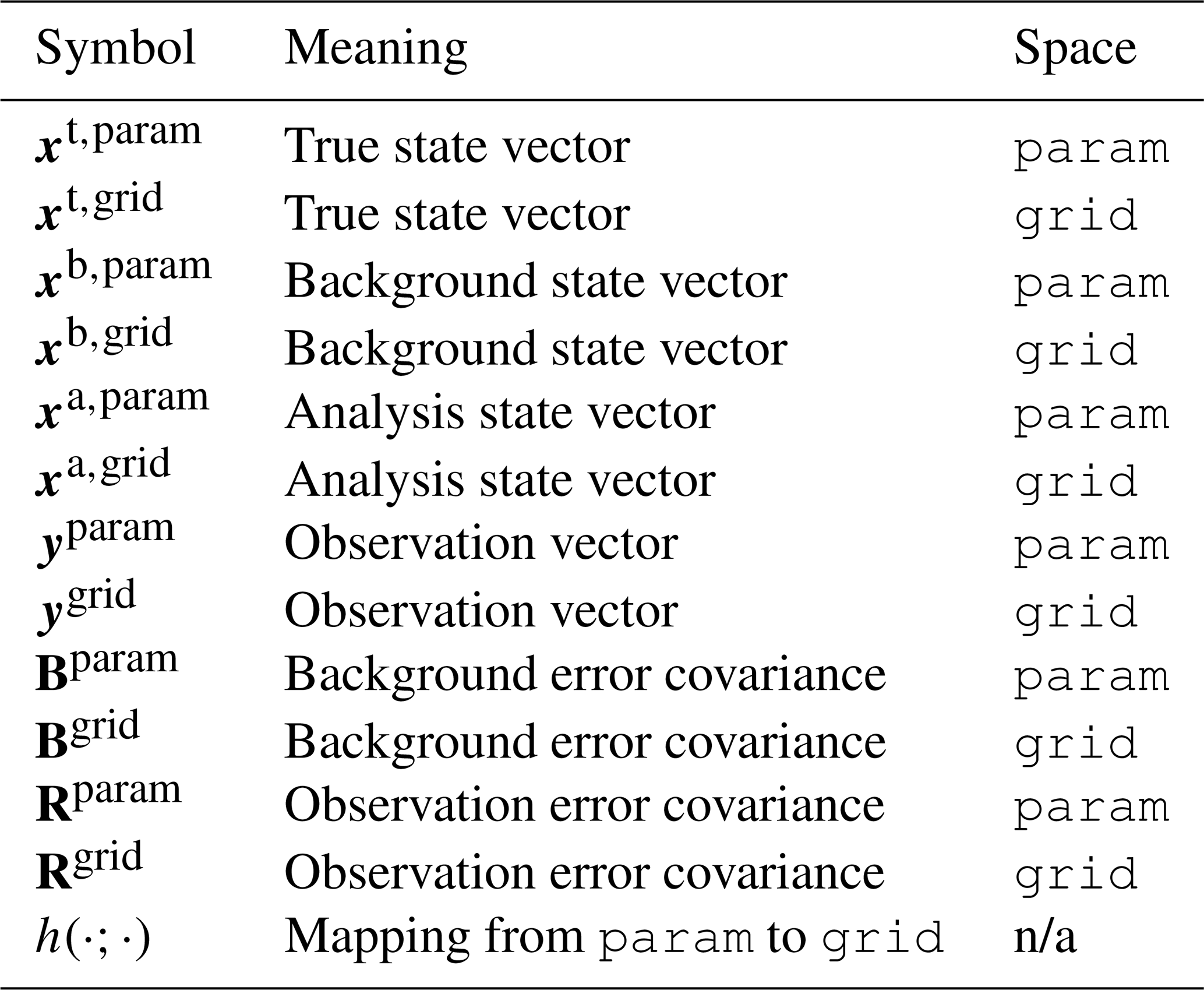
n/a: not space-specific, maps between spaces.

The background state in each space is modeled as a perturbation around a reference value:

$$\begin{array}{}\text{(2)}& {\displaystyle }{\displaystyle }\mathit{x}={\mathit{x}}^{\mathrm{b}}+{\mathit{\eta }}^{\mathrm{b}},\end{array}$$

where x^b is the reference background state and ${\mathit{\eta }}^{\mathrm{b}}\sim \mathcal{N}(\mathbf{0},\mathbf{B})$ is the background error, assumed Gaussian with covariance matrix B. The observation is related to the true state by:

$$\begin{array}{}\text{(3)}& {\displaystyle }{\displaystyle }\mathit{y}=\mathcal{H}\left(\mathit{x}\right)+\mathit{\epsilon },\end{array}$$

where ℋ is the observation operator and $\mathit{\epsilon }\sim \mathcal{N}(\mathbf{0},\mathbf{R})$ is the observation error with covariance R. Equations (2) and (3) are written generically and apply separately in each space with the appropriate superscript (param or grid) on all variables (see Table 1).

In our case, since the state vector is fully observed in both spaces, the operator ℋ is the identity matrix, leading to a simple linear observation equation.

The data assimilation is performed in each space with the appropriate superscript (param or grid) on all variables using the following cost function J:

$$\begin{array}{ll}{\displaystyle }J\left(\mathit{x}\right)=& {\displaystyle }{\displaystyle \frac{\mathrm{1}}{\mathrm{2}}}{\left(\mathit{x}-{\mathit{x}}^{\mathrm{b}}\right)}^{\mathrm{T}}{\mathbf{B}}^{-\mathrm{1}}\left(\mathit{x}-{\mathit{x}}^{\mathrm{b}}\right)\\ \text{(4)}& {\displaystyle }& {\displaystyle }+{\displaystyle \frac{\mathrm{1}}{\mathrm{2}}}(\mathit{y}-\mathit{x}{)}^{\mathrm{T}}{\mathbf{R}}^{-\mathrm{1}}(\mathit{y}-\mathit{x}).\end{array}$$

Under the assumptions of linearity and Gaussian errors, the minimizer of J is given analytically by the Best Linear Unbiased Estimator (BLUE). No iterative minimization algorithm is therefore required; the solution is computed directly for each configuration. Let ${\mathbf{X}}^{\mathrm{b}}=[{\mathit{x}}_{\mathrm{1}}^{\mathrm{b}},\mathrm{\dots },{\mathit{x}}_N^{\mathrm{b}}]$ and $\mathbf{Y}=[{\mathit{y}}_{\mathrm{1}},\mathrm{\dots },{\mathit{y}}_N]$ denote the background and observation ensemble matrices, each of size n×N (or m×N in grid space), where N is the ensemble size. The covariance matrices are estimated from these ensembles as:

$$\begin{array}{}\text{(5)}& {\displaystyle }{\displaystyle }\mathbf{B}=\text{Cov}({\mathbf{X}}^{\mathrm{b}},{\mathbf{X}}^{\mathrm{b}}),\text{ and }\mathbf{R}=\text{Cov}(\mathbf{Y},\mathbf{Y}),\end{array}$$

following the Ensemble Optimal Interpolation (EnOI) framework. The BLUE update of each ensemble member i reads:

$$\begin{array}{}\text{(6)}& {\displaystyle }{\displaystyle }{\mathit{x}}_i^{\mathrm{a}}={\mathit{x}}_i^{\mathrm{b}}+\mathbf{K}\left({\mathit{y}}_i-{\mathit{x}}_i^{\mathrm{b}}\right),i=\mathrm{1},\mathrm{\dots },N,\end{array}$$

from which the analysis ensemble mean ${\stackrel{\mathrm{‾}}{\mathit{x}}}^{\mathrm{a}}=\frac{\mathrm{1}}{N}{\sum }_i{\mathit{x}}_i^{\mathrm{a}}$ is derived, and the analysis error covariance P^a is given by:

$$\begin{array}{}\text{(7)}& {\displaystyle }{\displaystyle }{\mathbf{P}}^{\mathrm{a}}=(\mathbf{I}-\mathbf{K})\mathbf{B},\end{array}$$

where $\mathbf{K}=\mathbf{B}(\mathbf{B}+\mathbf{R}{)}^{-\mathrm{1}}$ is the Kalman gain. Equations (5)–(7) apply separately in each space with the appropriate superscript (param or grid) on all variables.

Two experimental frameworks are considered, differing in how the uncertainty is introduced and how the covariance matrices are specified, as described in the following subsections. In the tutorial framework (Sect. 2.1), the uncertainty originates in parameter space and is propagated to grid space via h. In the realistic framework (Sect. 2.2), the uncertainty originates in grid space and must be inverted back to parameter space through a fitting procedure, providing a more balanced end-to-end comparison.

2.1 Tutorial framework

This framework is designed as a controlled tutorial example to isolate the mechanism by which linear Gaussian updates can distort coherent structures in gridded space. It is not intended as a balanced end-to-end comparison of practical DA workflows, since the uncertainty is generated in parameter space and then mapped to grid space, which inherently favors the parametric approach.

In this framework, the parameters are assumed to be fully independent and to have equal uncertainties for both the background and the observation. The error covariance matrices in parameter space are therefore diagonal:

$$\begin{array}{}\text{(8)}& {\displaystyle }{\displaystyle }{\mathbf{B}}^{\text{param}}={\mathbf{R}}^{\text{param}}=\text{diag}({\mathit{\sigma }}_a^{\mathrm{2}},{\mathit{\sigma }}_p^{\mathrm{2}},{\mathit{\sigma }}_r^{\mathrm{2}})={\mathit{\sigma }}^{\mathrm{2}}{\mathbf{I}}_n,\end{array}$$

where σ=(σ_a, σ_p, σ_r) contains the prescribed standard deviations for amplitude, position and radius, respectively.

Ensemble members in param space are generated by independently sampling each parameter from a Gaussian distribution around its reference value with the prescribed standard deviation. The corresponding ensemble members in grid space are then obtained by applying the mapping h (Eq. 1) to each member, so that the gridded covariance matrices B^grid and R^grid are fully determined by the nonlinear push-forward of the parametric uncertainties. As a result, these gridded covariances are in general non-diagonal and reflect the nonlinear geometry of the eddy profile, even though the parametric uncertainties are uncorrelated.

An analytic alternative to this ensemble-based propagation would be a first- or second-order Taylor expansion of h around the reference parameter vector. We tested this local linearization and found it inadequate in the nonlinear regime relevant to this study. Because $\partial h/\partial p$ vanishes at the profile peak by symmetry, the Taylor-propagated standard deviation drops to zero with a slope discontinuity at that location for both prior covariance matrices, B^grid and R^grid, each centered on its own reference position ($p=-\mathrm{5}$ and $p=+\mathrm{5}$ km, respectively, in Experiment #2, see Sect. 3.1). In contrast, the Monte Carlo ensemble produces a smooth, non-zero local minimum there, reflecting the non-Gaussian structure induced by a displacement comparable to the eddy radius. More critically, when the background and observation are linearized separately around distinct mean positions, the resulting covariance matrices are rank-deficient and mutually asymmetric; the corresponding Kalman gain produces an unphysical negative undershoot in the analyzed height over a substantial fraction of the domain, and the posterior covariance to collapse to numerically negligible values almost everywhere (Appendix A, Fig. A1). The ensemble (Monte Carlo) approach described above does not exhibit this pathology and was therefore retained throughout this study.

Figure 1 illustrates the overall workflow comparing assimilation in the parametric and gridded spaces.

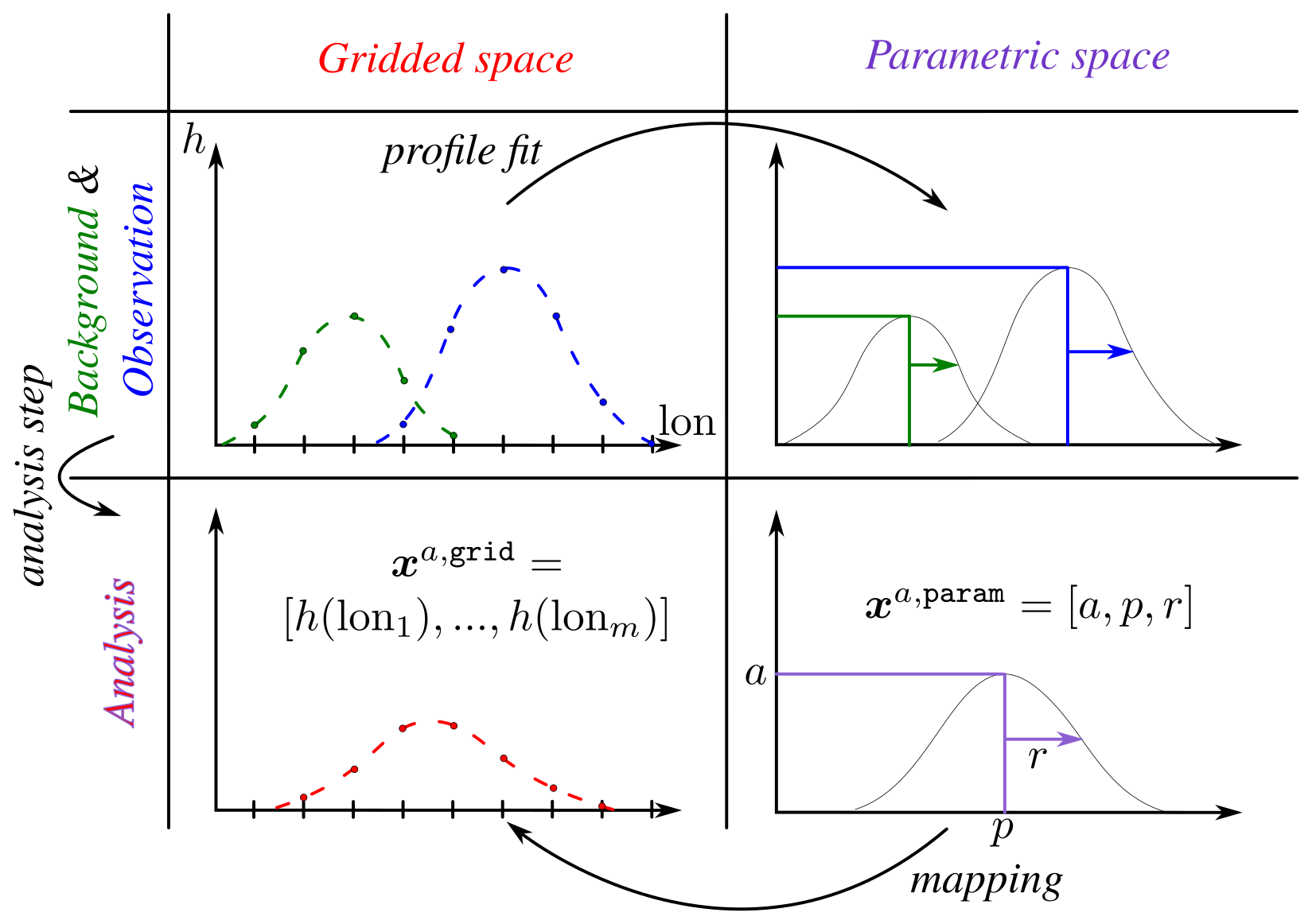
Figure 1 Schematic of the data assimilation framework comparing gridded space (left column, red) and parametric space (right column, purple). Top row: background (green) and observation (blue) eddies represented as gridded profiles (top left) and as parameter vectors (top right). The profile fit arrow indicates the nonlinear least-squares mapping from gridded observations to parameter space, as used in Experiment #4. Bottom row: analysis state from the analysis step in gridded space ${\mathit{x}}^{\mathrm{a},\text{grid}}=\left[h\right({\text{lon}}_{\mathrm{1}}),\mathrm{\dots },h({\text{lon}}_m\left)\right]$ (bottom left) and in parametric space x^a,param (bottom right). The mapping arrow indicates the projection of the parametric analysis back to gridded space via h (Eq. 1).

2.2 Realistic framework

In realistic applications, observations are available as gridded fields rather than direct eddy parameters. In this second framework, both the background and the observation start as noisy gridded profiles, and the parametric representation must be inferred from them through a fitting procedure. This constitutes a more balanced end-to-end test, since the uncertainty now originates in grid space and the inverse nonlinear mapping from grid to parameter space is explicitly accounted for.

The observed and background gridded fields are defined as:

$$\begin{array}{}\text{(9)}& {\displaystyle }& {\displaystyle }{\mathit{y}}^{\text{grid}}=h\left(\mathbf{lon};{\mathit{y}}^{\text{param},\star }\right)+{\mathit{\epsilon }}^{\text{grid}},\text{(10)}& {\displaystyle }& {\displaystyle }{\mathit{x}}^{\mathrm{b},\text{grid}}=h\left(\mathbf{lon};{\mathit{x}}^{\mathrm{b},\text{param},\star }\right)+{\mathit{\eta }}^{\mathrm{b},\text{grid}},\end{array}$$

where ${\mathit{y}}^{\text{param},\star }$ and ${\mathit{x}}^{\mathrm{b},\text{param},\star }$ are the reference observation and background parameter vectors, and ${\mathit{\epsilon }}^{\text{grid}}\sim \mathcal{N}(\mathbf{0},{\mathbf{R}}^{\text{grid}})$, ${\mathit{\eta }}^{\mathrm{b},\text{grid}}\sim \mathcal{N}(\mathbf{0},{\mathbf{B}}^{\text{grid}})$ are the respective gridded noise terms. The gridded covariance matrices are prescribed using an exponentially decaying correlation model:

$$\begin{array}{}\text{(11)}& {\displaystyle }{\displaystyle }{\mathbf{B}}_{ij}^{\text{grid}}={\mathbf{R}}_{ij}^{\text{grid}}={\mathit{\sigma }}_h^{\mathrm{2}}\exp \left(-{\displaystyle \frac{|{\text{lon}}_i-{\text{lon}}_j|}{\mathit{\lambda }}}\right),\end{array}$$

where ${\mathit{\sigma }}_h^{\mathrm{2}}$ is the surface-height variance and λ is the correlation length scale. In the gridded DA approach, y^grid is assimilated directly using Eqs. (6)–(7) with these prescribed covariances.

For the parametric DA approach, the parameter vectors are first estimated from the noisy gridded fields through a nonlinear least-squares fit of the Gaussian profile h. Specifically, for a given noisy gridded profile u, the estimated parameter vector $\widehat{\mathit{\theta }}$ minimizes:

$$\begin{array}{}\text{(12)}& {\displaystyle }{\displaystyle }\mathcal{L}\left(\mathit{\theta }\right)={∥\mathit{u}-h(\mathbf{lon};\mathit{\theta })∥}_{\mathrm{2}}^{\mathrm{2}}.\end{array}$$

The minimization is performed using the scipy.optimize.curve_fit algorithm with bounds $a\in [\mathrm{0},\mathrm{10}]$ m, $p\in [-\mathrm{50},\mathrm{50}]$ km, and $r\in [\mathrm{0.1},\mathrm{50}]$ km, ensuring physical solutions (positive amplitude and positive radius). The initial values for the fit are set as following: $[max\mathit{u},{\mathbf{lon}}_{\arg max\mathit{u}},\frac{\mathrm{1}}{\mathrm{2}}\left|{\mathbf{lon}}_{\arg max\mathit{u}}-{\mathbf{lon}}_{\arg min\mathit{u}}\right|]$ where the amplitude is initialized from the maximum value of the profile, the center from the longitude at which this maximum occurs, and the width from half the distance between the longitudes of the maximum and minimum values. This simplified initialization is appropriate given the idealized framework of the present experiment. In practice, initial values could be provided by a prior detection algorithm.

The fitting procedure is repeated over an ensemble of N noisy realizations drawn from Eqs. (9)–(10). The parametric covariance matrices are then estimated as the sample covariance of the fitted parameter ensembles, determined by the nonlinear push-forward of the gridded height uncertainties. Unlike the tutorial framework, these covariance matrices are in general non-diagonal, reflecting the nonlinear coupling between parameters introduced by the fitting procedure. The parametric DA is then performed using Eqs. (6) and (7) in param space with these estimated covariances.

3 Experiments

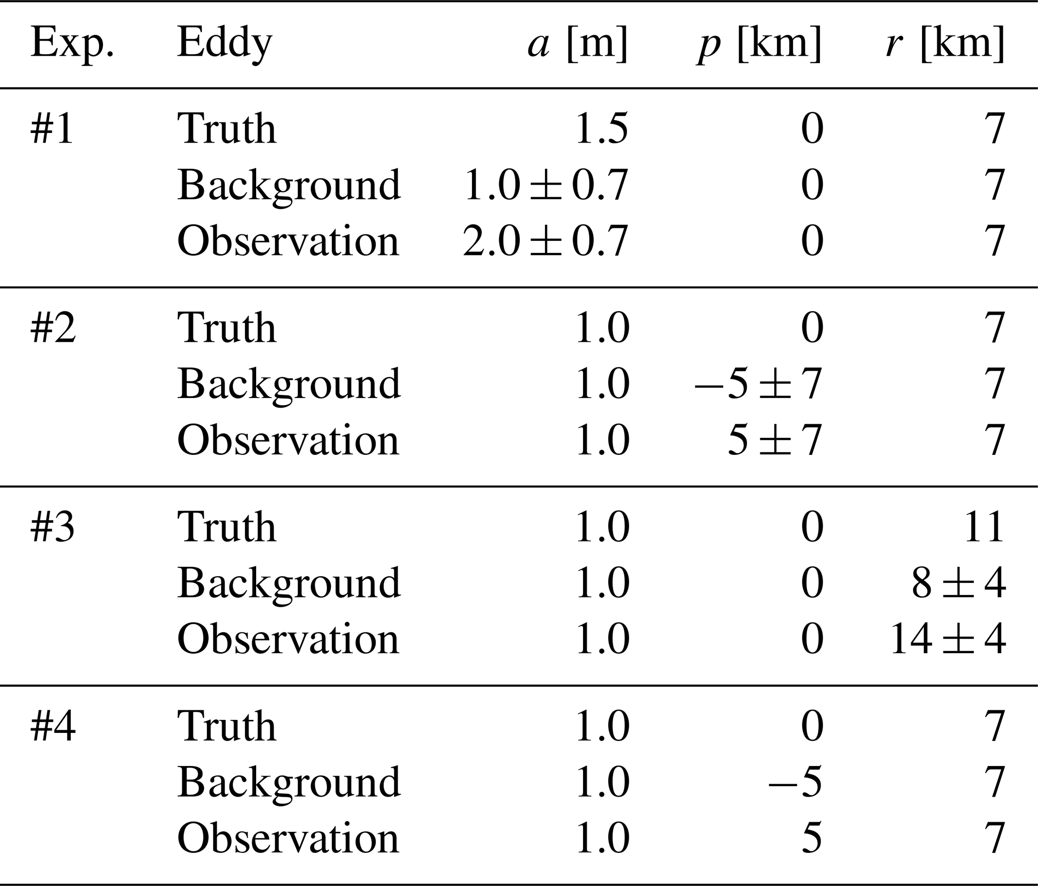
Four experiments are presented, organized into two sets corresponding to the two frameworks described in Sect. 2. Experiments #1, #2, and #3 follow the tutorial framework (Sect. 2.1) and are designed to isolate the effect of a single uncertain parameter on the assimilation outcome. Experiment #4 follows the realistic framework (Sect. 2.2) and provides a more balanced end-to-end evaluation by starting from noisy gridded observations. The parameter values for all four experiments are given in Table 2.

Table 2 True parameter values x^t,param and reference parameter values with prescribed standard deviations (±σ) for the background and observation in each experiment. The background and observation are constructed symmetrically around the truth via Eq. (13). For Experiment #4, no standard deviation is prescribed in parameter space; the uncertainty is instead introduced as additive gridded noise with amplitude σ_h=0.2 m and correlation length $\mathit{\lambda }=r/\mathrm{2}=\mathrm{3.5}$ km (see Sect. 2.2).

3.1 Tutorial experiments (#1, #2, #3)

In each of the three tutorial experiments, a single parameter carries the uncertainty, while the other two are set to their true values and are identical in the background and the observation. The uncertain parameter is, respectively: amplitude a (Experiment #1), position p (Experiment #2), and radius r (Experiment #3). This design isolates the effect of each parameter's nonlinearity on the assimilation update (see Table 2).

This setup inherently favors the parametric approach (Sect. 2.1); these experiments therefore isolate the mechanism by which a nonlinearly entering parameter causes gridded-space updates to smear the structure, rather than providing a balanced workflow comparison.

The background and observation are constructed symmetrically around a true state x^t,param by applying shifts of equal magnitude and opposite sign:

$$\begin{array}{}\text{(13)}& {\displaystyle }{\displaystyle }{\mathit{x}}^{\mathrm{b},\text{param}}={\mathit{x}}^{\mathrm{t},\text{param}}-\mathit{\delta },\text{and}{\mathit{y}}^{\text{param}}={\mathit{x}}^{\mathrm{t},\text{param}}+\mathit{\delta },\end{array}$$

where δ is the prescribed shift vector, with only the uncertain parameter having a non-zero component. The associated true gridded profile is ${\mathit{x}}^{\mathrm{t},\text{grid}}=h(\mathbf{lon};{\mathit{x}}^{\mathrm{t},\text{param}})$. This symmetric construction ensures that the background and observation errors are equal in magnitude, so that the expected BLUE analysis in parameter space recovers the truth exactly: ${\stackrel{\mathrm{‾}}{\mathit{x}}}^{\mathrm{a},\text{param}}={\mathit{x}}^{\mathrm{t},\text{param}}$.

An ensemble of N=10 000 members is used for both the background and the observation. In param space, ensemble members are generated by independently sampling each parameter from a Gaussian distribution around its reference value with the prescribed standard deviation σ_a, σ_p, or σ_r (the non-perturbed parameters having zero spread). The corresponding grid ensemble members are obtained by applying h (Eq. 1) to each parametric member, as described in Sect. 2.1. The radius is clipped to $r\ge {\mathrm{10}}^{-\mathrm{6}}$ km to prevent non-physical values.

3.2 Realistic experiment (#4)

Experiment #4 uses the same reference parameter values as Experiment #2 (position perturbation), but the uncertainty is now introduced directly in grid space following the realistic framework of Sect. 2.2. The background and observation gridded fields are generated as:

$$\begin{array}{ll}{\displaystyle }& {\displaystyle }{\mathit{x}}^{\mathrm{b},\text{grid}}=h(\mathbf{lon};(-\mathrm{5},\mathrm{1},\mathrm{7}\left)\right)+{\mathit{\eta }}^{\mathrm{b},\text{grid}},\text{and}\\ \text{(14)}& {\displaystyle }& {\displaystyle }{\mathit{y}}^{\text{grid}}=h(\mathbf{lon};(\mathrm{5},\mathrm{1},\mathrm{7}\left)\right)+{\mathit{\epsilon }}^{\text{grid}},\end{array}$$

where the noise terms are drawn from the exponentially correlated distribution of Eq. (11) with σ_h=0.2 m and $\mathit{\lambda }=r/\mathrm{2}=\mathrm{3.5}$ km.

For the parametric DA, an ensemble of N=10 000 noisy realizations is generated for both the background and the observation. Each realization is fitted independently using the procedure described in Sect. 2.2, yielding an ensemble of parameter vectors from which B^param and R^param are estimated. To assess the robustness of the results with respect to the noise realization, the full experiment is repeated n_iter=10 times with independent noise draws; quantitative diagnostics are reported as means and standard deviations over these 10 noise realizations.

3.3 Evaluation

For all four experiments, two comparisons are performed:

• Surface height reconstruction: The analysis mean is projected into grid space and compared to the true profile x^t,grid. For the parametric analysis, the projection is done by applying h (Eq. 1) to the analyzed parameter vector ${\stackrel{\mathrm{‾}}{\mathit{x}}}^{\mathrm{a},\text{param}}$. For the gridded analysis, the profile ${\stackrel{\mathrm{‾}}{\mathit{x}}}^{\mathrm{a},\text{grid}}$ is used directly. Two metrics are reported: the Root Mean Square Error (RMSE) of the analysis mean relative to x^t,grid, and the Continuous Ranked Probability Score (CRPS) of the analysis ensemble relative to x^t,grid, which jointly measures accuracy and sharpness of the probabilistic forecast.

• Parameter estimation: The estimated parameters of each analysis are compared to the true values x^t,param. For the parametric analysis, the estimated parameters are directly ${\stackrel{\mathrm{‾}}{\mathit{x}}}^{\mathrm{a},\text{param}}$. For the gridded analysis, the analyzed profile is fitted with the Gaussian function h using the least-squares procedure of Eq. (12), yielding estimated parameters ${\widehat{\mathit{\theta }}}^{\text{grid}}$. The absolute error of each analysis relative to the truth is reported for each parameter separately, defined as $|{\widehat{\mathit{\theta }}}_k^{\text{grid}}-x_k^{\mathrm{t},\text{param}}|$ and $|{\stackrel{\mathrm{‾}}{x}}_k^{\mathrm{a},\text{param}}-x_k^{\mathrm{t},\text{param}}|$ for $k\in \mathit{\{}a,p,r\mathit{\}}$.

4 Results and discussion

4.1 Tutorial experiments (#1, #2, #3)

The surface height profiles are shown in Figs. 2–4 for the amplitude, position and radius perturbation experiments, respectively. The quantitative diagnostics for all experiments are reported in Tables 3 and 4.

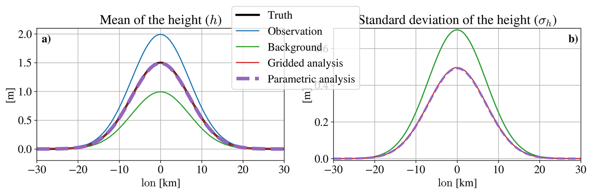
Figure 2 Results for Experiment #1 (amplitude perturbation). (a) True surface height (black), mean surface height of the observed (blue), background (green), gridded analysis (red), and parametric analysis (dashed purple) eddies along the longitude. (b) Corresponding a posteriori standard deviation ${\mathit{\sigma }}_h=\sqrt{\text{diag}\left({\mathbf{P}}^{\mathrm{a}}\right)}$.

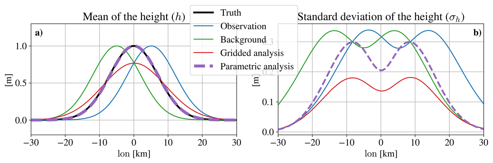
Figure 3 Results for Experiment #2 (position perturbation). Same color and panel convention as Fig. 2.

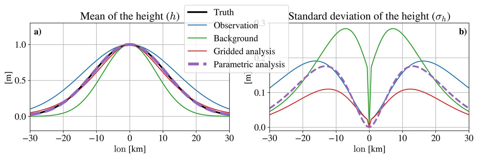
Figure 4 Results for Experiment #3 (radius perturbation). Same color and panel convention as Fig. 2.

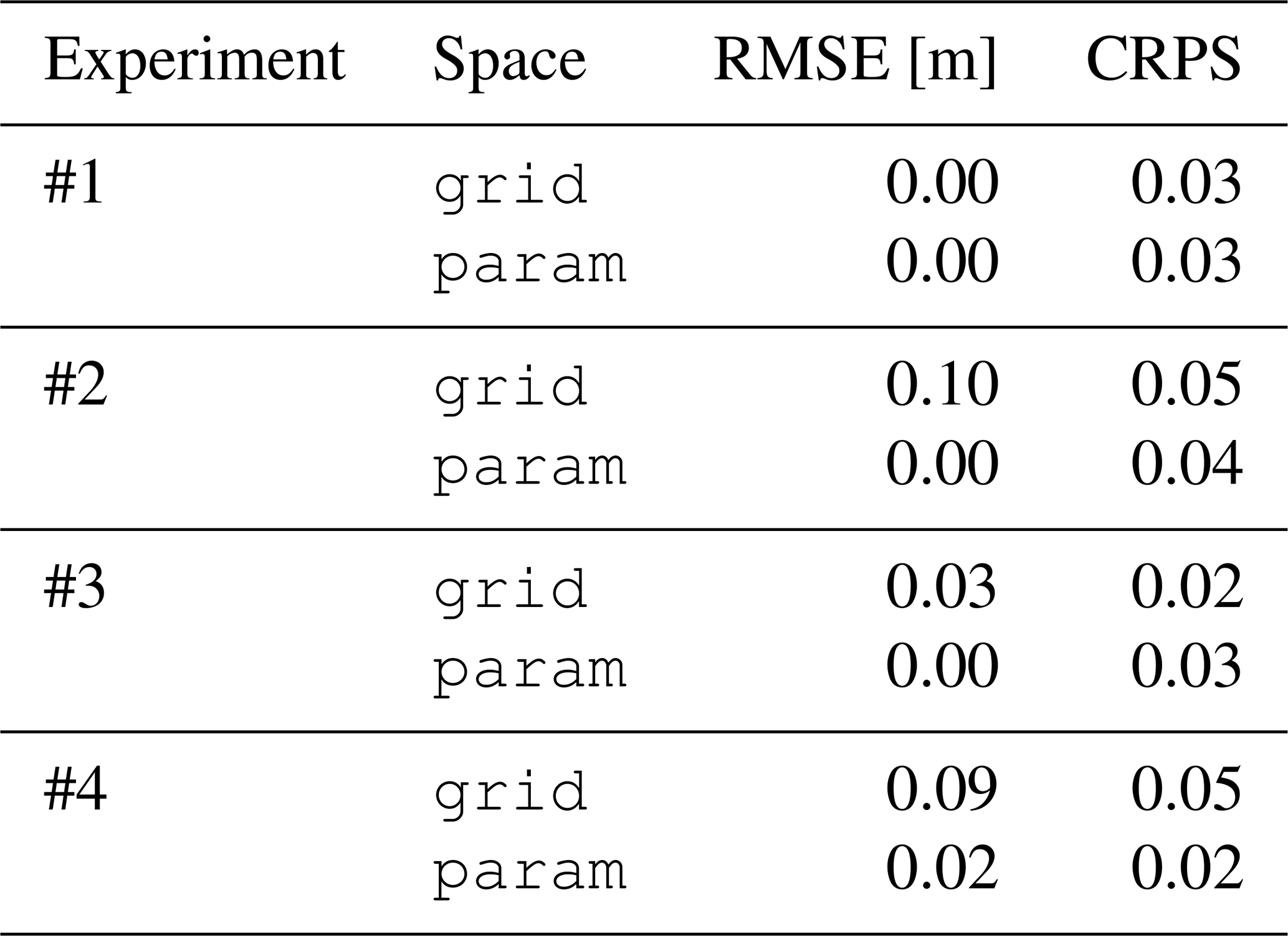
Table 3 Gridded field diagnostics for all experiments. RMSE: root-mean squared error of the analysis mean relative to the true profile x^t,grid (lower is better); CRPS: continuous ranked probability score of the analysis ensemble relative to x^t,grid (lower is better). For Experiment #4, values are means over 10 noise realizations.

Experiment #1 – Amplitude perturbation

Figure 2a shows that the analyzed profiles are identical in both param and grid spaces: the analyzed amplitude is 1.5 m, the exact mean of the background (1.0 m) and observation (2.0 m), with position and radius unchanged. Figure 2b shows identical a posteriori standard deviation profiles in both spaces. This agreement reflects the fact that amplitude is a linear parameter of h (Eq. 1): the nonlinear push-forward that distinguishes the two approaches has no effect in this case.

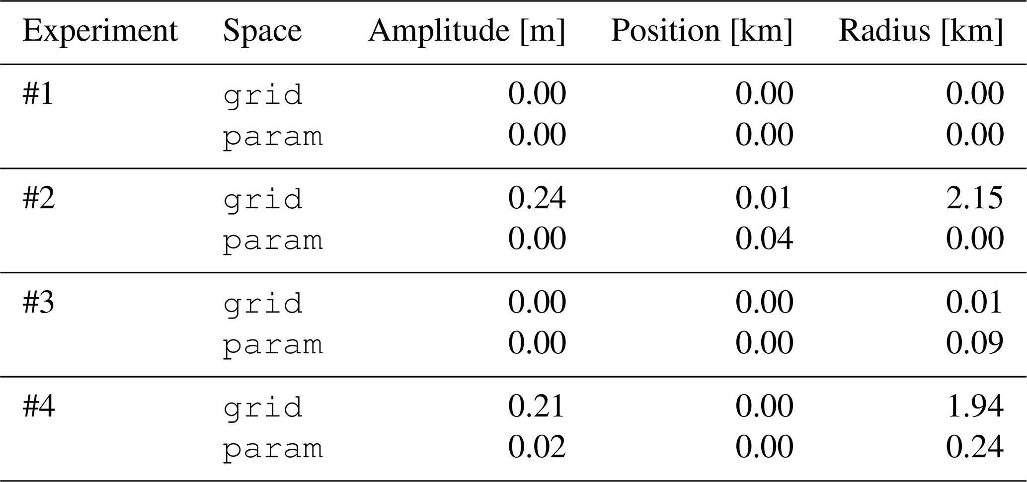
This is confirmed by the metrics in Table 3: the RMSE is 0.00 in both spaces, and the CRPS values are 0.03. The absolute error is 0.00 for all parameters (see Table 4).

Table 4 Parameter estimation diagnostics for all experiments. Values are the signed errors of the analyzed parameters relative to the truth x^t,param: $|{\widehat{\mathit{\theta }}}_k^{\text{grid}}-x_k^{\mathrm{t},\text{param}}|$ for the gridded analysis (after Gaussian fitting) and $|{\stackrel{\mathrm{‾}}{x}}_k^{\mathrm{a},\text{param}}-x_k^{\mathrm{t},\text{param}}|$ for the parametric analysis, for $k\in \mathit{\{}a,p,r\mathit{\}}$. For Experiment #4, values are means over 10 noise realizations.

Experiment #2 – Position perturbation

By contrast, Fig. 3a shows a clear difference between the two analyses. The grid analyzed profile is widened and flattened relative to both the background and the observation. A Gaussian fit of this profile yields $(a,p,r)$ ≈ (0.77 m, 0.02 km, 9.05 km): the amplitude is underestimated by 23 % and the radius overestimated by 29 % relative to the true values, even though the position is correctly recovered. This deformation is a direct consequence of the nonlinear dependence of h on position: the linear Gaussian update in grid space averages the two displaced profiles, producing a broader, lower peak, rather than a correctly shaped one.

In contrast, the param analysis recovers $(a,p,r)$ = (1.0 m, 0.0 km, 7.0 km), the exact midpoint in parameter space, with all three parameters correctly estimated. The a posteriori standard deviation in grid space (Fig. 3b) is also spatially underestimated relative to the param counterpart, indicating that the gridded analysis is overconfident about the reconstructed profile.

These differences are captured by the metrics: the RMSE increases to 0.10 m in the grid space, while it remains at 0.00 m in the param space. The CRPS is slightly better in the param space. The absolute error shows higher values for the estimation of the amplitude (0.24 m) and the radius (2.15 km) in the grid space, while the position is well-estimated (Table 4).

Experiment #3 – Radius perturbation

Figure 4a shows that the grid analyzed profile has a narrower peak with a wider tail, compared to the param profile. A Gaussian fit yields $(a,p,r)$ ≈ (0.96 m, 0.00 km, 11.09 km): the radius is correctly recovered (11.09 km, close to the expected mean of 11 km), but the amplitude is slightly underestimated (0.96 m vs. 1.0 m). More importantly, the grid analyzed profile is no longer strictly Gaussian: the profile shape is sub-Gaussian, with a narrower core and heavier tails than a Gaussian of the same standard deviation, a consequence of the nonlinear averaging of two Gaussian profiles of different widths in grid space. In the param space, the estimated radius is 11 km (the mean of 8 and 14 km) and the profile remains Gaussian. The grid RMSE is slightly higher (0.03 m), while the CRPS value is close (0.02 for the grid space and 0.03 for the param space).

4.2 Realistic experiment (#4)

Figure 5 shows the results for Experiment #4. The qualitative behavior is consistent with Experiment #2: the grid analysis produces a widened and underestimated profile (Gaussian fit: a≈0.79 m, p≈0.04 km, r≈8.96 km), while the param analysis recovers parameters close to the expected mean. These values are stable across the 10 noise realizations.

Figure 5 Results for Experiment #4 (realistic framework, position perturbation). Same color and panel convention as Fig. 2. Results are shown for a representative single noise realization; quantitative diagnostics in Tables 3 and 4 are means over 10 noise realizations.

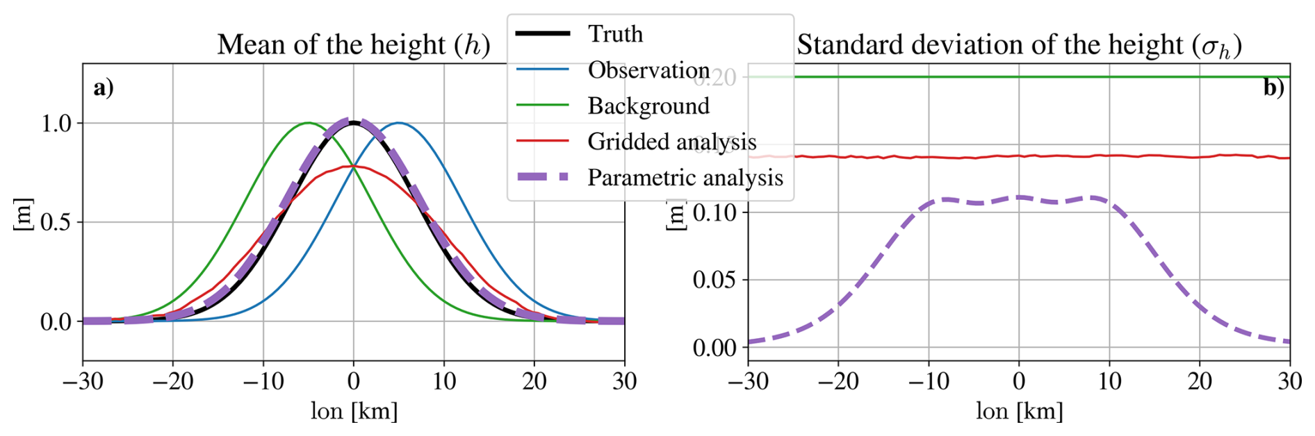
The a posteriori standard deviations differ from Experiment #2 (Fig. 5b). In the grid space, the standard deviation is spatially uniform at approximately $\mathrm{0.2}/\sqrt{\mathrm{2}}$ m, reflecting the prescribed exponentially correlated noise structure. In the param space, the standard deviation is spatially varying, with larger values in the region spanned by the background and observation positions: this spatial structure directly reflects the positional uncertainty of the eddy, and is a distinctive feature of the parametric representation.

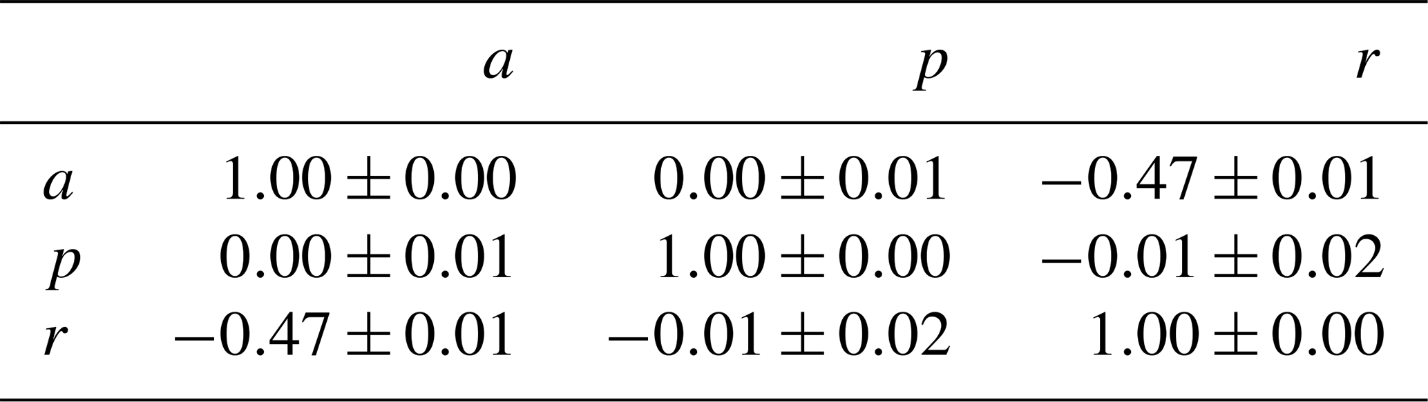
The mean correlation matrix of the fitted parameters, estimated over the 10 noise realizations, is reported in Table 5. The dominant off-diagonal correlation is between amplitude a and radius r ($-\mathrm{0.47}\pm \mathrm{0.01}$): wider fits tend to produce lower peak amplitudes, reflecting a geometric coupling introduced by the nonlinear fitting procedure. The correlation between position p and the other parameters is negligible ($<\left|\mathrm{0.01}\right|$), consistent with the symmetry of the Gaussian profile. This non-diagonal covariance structure means that B^param and R^param are no longer diagonal, unlike in the tutorial experiments.

Table 5 Mean parameter correlation matrix ${\stackrel{\mathrm{‾}}{\mathbf{P}}}^{\mathrm{a},\text{param}}$ estimated from the fitting ensemble, averaged over 10 noise realizations (Experiment #4). Values are mean and standard deviations across realizations.

After assimilation, the posterior covariance P^a,param shows variances approximately halved relative to the prior, consistent with the expected uncertainty reduction for equal background and observation errors. Diagnostic tests on the fitted parameter ensembles further reveal that this fitting-induced structure is not fully Gaussian: the radius parameter, in particular, shows significant skewness and excess kurtosis (Shapiro–Wilk normality test $p<{\mathrm{10}}^{-\mathrm{30}}$), although the ensemble mean used by the EnOI update exhibits only a small bias relative to the generating value.

The metrics for Experiment #4 (Tables 3 and 4) confirm the qualitative observations. The RMSE increases to 0.09 m in grid (compared to 0.02 m in the param space). The CRPS in both spaces remains low, with still a higher difference between the grid space (0.05) and the param space (0.02). The parameter estimation in the grid space shows similar values compared to Experiment #2, with slightly improved performance (0.21 m instead of 0.24 m for the amplitude and 1.94 km instead of 2.15 km for the radius). Compared with the analytically prescribed covariance, estimating the parameter covariance from a noisy fitting procedure results in larger errors for the amplitude (0.02 m) and radius (0.24 km).

Overall, Experiment #4 shows that the parametric approach recovers the coherent structure properties when starting from noisy gridded observations.

4.3 Physical illustration: Eddy Kinetic Energy

The profile deformations observed in Experiments #2, #3, and #4 have consequences for the physical properties of the reconstructed eddy. As an illustration of this effect, we compute the geostrophic velocity and associated Eddy Kinetic Energy (EKE) from the analyzed height profiles. The geostrophic velocity is given by:

$$\begin{array}{}\text{(15)}& {\displaystyle }{\displaystyle }{v}_{\mathrm{g}}\left(x\right)=-{\displaystyle \frac{g}{f}}{\displaystyle \frac{\partial h}{\partial x}},\end{array}$$

where g=9.81 m s⁻² is gravitational acceleration and $f={\mathrm{10}}^{-\mathrm{4}}$ s⁻¹ is the Coriolis parameter. The EKE per unit volume and the total integrated EKE are then:

$$\begin{array}{ll}{\displaystyle }& {\displaystyle }\text{EKE}\left(x\right)={\displaystyle \frac{\mathit{\rho }}{\mathrm{2}}}{v}_{\mathrm{g}}(x{)}^{\mathrm{2}},\\ \text{(16)}& {\displaystyle }& {\displaystyle }{\text{EKE}}_{\text{tot}}=\underset{\text{lon}}{\int }\text{EKE}\left(x\right)\mathrm{d}x,\end{array}$$

with ρ=1000 kg m⁻³.

This diagnostic is not used here as a validation metric, but as a concrete illustration of how structural distortions in the gridded analysis propagate into physically relevant quantities. Because EKE scales as the square of the height gradient, even moderate profile deformations can have a disproportionate impact on this quantity. Values are given in Table 6.

Table 6 EKE [kJ m⁻²]: total integrated eddy kinetic energy computed from the analysis mean profile, reported as a physical illustration. For Experiment #4, values are means over 10 noise realizations.

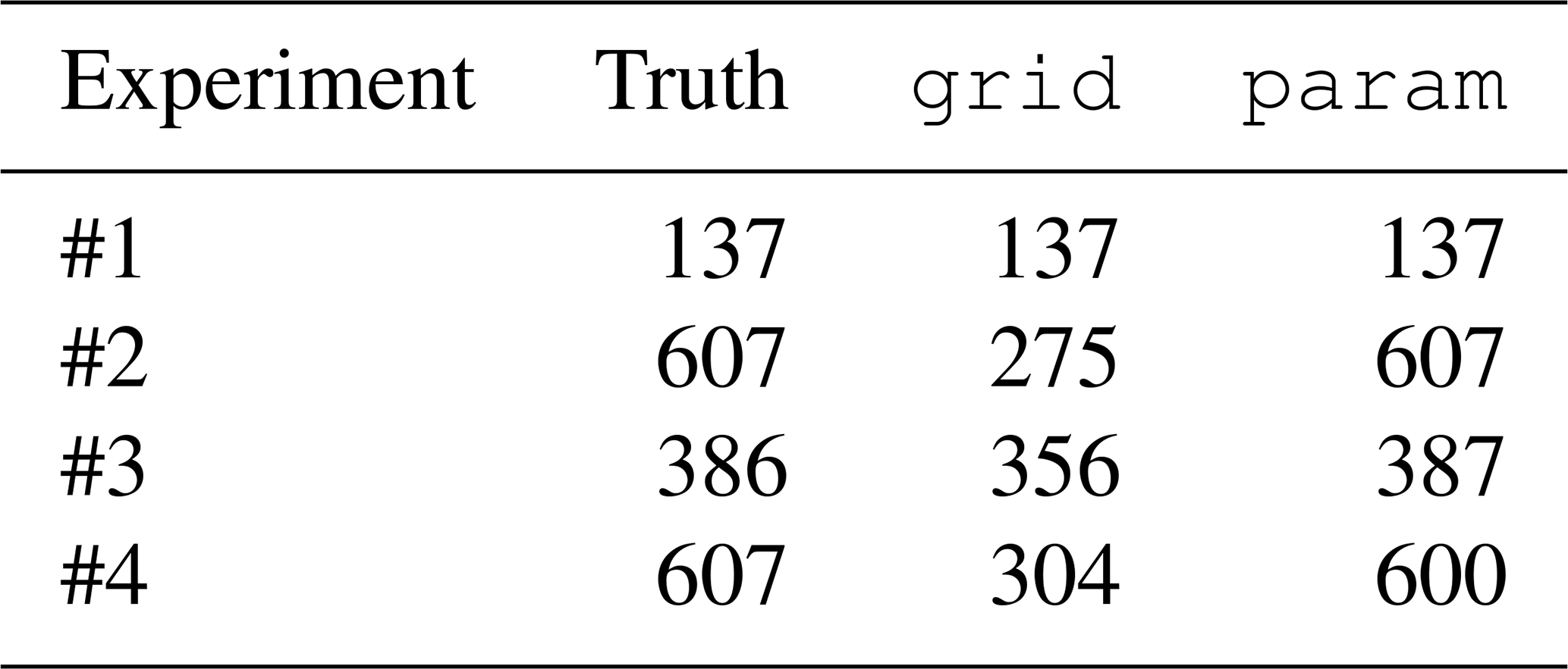
In Experiment #2, the widened and flattened grid analyzed profile produces smaller height gradients and therefore weaker geostrophic currents. The resulting total EKE is reduced by 55 % relative to the value computed from the true profile. In Experiment #3, the sub-Gaussian shape similarly reduces the peak gradient, leading to an 8 % reduction in total EKE relative to the true value. For both experiments, EKE estimations from the param projected profile have the same values as the truth. Similarly to Experiment #2, the flattened grid analyzed profile induces an EKE reduction of 50 % while the slightly lower peak of the param projected profile reduces the EKE by only 1 %. These reductions would directly affect estimates of lateral transport, air-sea interactions, and the mesoscale energy budget.

4.4 Computational complexity

We provide a theoretical, order-of-magnitude comparison of the computational costs associated with the Eulerian, Arbitrary Lagrangian–Eulerian (ALE) (Hirt et al., 1974), and parametric representations considered in this study. This is not intended as a numerical benchmark, since a fair comparison of wall-clock times would require complete implementations of the three approaches.

Consider a coherent structure of characteristic radius r in a domain of size L, discretized with a numerical scheme of order q, the relative discretization error scales as

$$\begin{array}{}\text{(17)}& {\displaystyle }{\displaystyle }\mathit{\epsilon }\sim {\left({\displaystyle \frac{\mathrm{\Delta }\mathbf{lon}}{r}}\right)}^q,\end{array}$$

so that the grid spacing required to achieve a tolerance ε scales as

$$\begin{array}{}\text{(18)}& {\displaystyle }{\displaystyle }\mathrm{\Delta }\mathbf{lon}\sim r{\mathit{\epsilon }}^{\mathrm{1}/q}.\end{array}$$

In d dimensions, the number of grid points per spatial direction is $L/\mathrm{\Delta }\mathbf{lon}\sim (L/r){\mathit{\epsilon }}^{-\mathrm{1}/q}$, so a fixed Eulerian grid covering the full domain therefore requires

$$\begin{array}{}\text{(19)}& {\displaystyle }{\displaystyle }{m}_{\text{Eulerian}}\left(d\right)\sim (L/r{)}^d{\mathit{\epsilon }}^{-d/q},\end{array}$$

degrees of freedom.

An ALE representation (Aydøğdu et al., 2019), which concentrates the resolution around each of K tracked structures, requires instead

$$\begin{array}{}\text{(20)}& {\displaystyle }{\displaystyle }{m}_{\text{ALE}}\left(d\right)\sim K{c}^d{\mathit{\epsilon }}^{-d/q},\end{array}$$

where c=O(1) characterizes the size of the refined region relative to the structure radius.

The parametric representation used here reduces the state to n_param=3K parameters, independently of the grid resolution and physical dimension. Thus, in terms of state dimension, the parametric representation is substantially smaller than both the Eulerian and ALE representations.

The computational cost of the assimilation step nevertheless depends on the ensemble size and on the dimension of the state being updated. For an ensemble-based linear update implemented in the N-dimensional ensemble subspace, rather than by explicitly forming and inverting the full m×m covariance matrix (e.g. via the Sherman–Morrison–Woodbury identity), a representative scaling is O(N²m) (Evensen, 2003; Nino Ruiz et al., 2015), compared to O(m³) for a direct, non-ensemble-subspace implementation. The corresponding costs therefore scale as

$$\begin{array}{ll}{\displaystyle }& {\displaystyle }{C}_{\text{Eulerian}}=O\left(N^{\mathrm{2}}{m}_{\text{Eulerian}}\right),\\ \text{(21)}& {\displaystyle }& {\displaystyle }{C}_{\text{ALE}}=O\left(N^{\mathrm{2}}{m}_{\text{ALE}}\right),\end{array}$$

whereas the parametric analysis itself costs only

$$\begin{array}{}\text{(22)}& {\displaystyle }{\displaystyle }{C}_{\text{param}}=O\left(N^{\mathrm{2}}{n}_{\text{param}}\right).\end{array}$$

The parametric approach, however, requires an additional parameter-extraction step before the analysis. In the present framework, each ensemble member is fitted to the parametric structure using nonlinear least squares (Eq. 12). If m denotes the resolution of the input grid, the cost of this step can be approximated as

$$\begin{array}{}\text{(23)}& {\displaystyle }{\displaystyle }{C}_{\text{fit}}=O\left(Nm{n}_{\text{iter}}\right),\end{array}$$

where m is the resolution of the input grid and n_iter is the number of nonlinear solver iterations. The total cost of the proposed approach is therefore

$$\begin{array}{}\text{(24)}& {\displaystyle }{\displaystyle }{C}_{\text{total,param}}=O\left(Nm{n}_{\text{iter}}+N^{\mathrm{2}}{n}_{\text{param}}\right).\end{array}$$

This comparison highlights the main computational trade-off of the proposed representation. The analysis step becomes substantially cheaper because it is performed in a low-dimensional parameter space, but this reduction comes at the expense of the additional parameter-extraction step applied to each ensemble member. The overall computational benefit therefore depends on the relative cost of these two stages, and hence on the grid resolution, the ensemble size, and the cost of the nonlinear fit.

5 Conclusions

This study investigates data assimilation (DA) performed in a reduced parametric space as well as classic linear and Gaussian DA in gridded space, focusing on a simplified one-dimensional representation of an ocean eddy and on a single analysis step.

The results obtained in this idealized framework indicate that DA in gridded space provides satisfactory reconstructions when uncertainty mainly affects linear parameters such as amplitude, as illustrated by Experiment #1, where both approaches yield identical results (RMSE = 0.00 m, zero parameter error). However, when uncertainty involves nonlinear geometric parameters such as position and radius, the gridded-space update leads to a deformation of the reconstructed structure. In Experiment #2, the gridded analysis underestimates the amplitude by 23 % (error of 0.24 m) and overestimates the radius by 29 % (error of 2.15 km), while the RMSE relative to the true profile reaches 0.10 m, compared with 0.00 m in parametric space. In Experiment #3, the analyzed profile is no longer Gaussian, and the RMSE in gridded space (0.03 m) exceeds that in parametric space (0.00 m). These structural distortions affect derived physical quantities: the total EKE is reduced by 67 % in Experiment #2 and by 11 % in Experiment #3 relative to the parametric analysis. These EKE figures are reported as an illustration of the physical consequences of the profile deformation, rather than as validation metrics.

The tutorial experiments (#1–3) are useful to isolate and illustrate this mechanism, but they do not constitute a balanced end-to-end comparison, since the uncertainty originates in parameter space and is propagated to grid space. Experiment #4, which starts from noisy gridded observations, provides a more symmetric test. The parametric approach retains its qualitative advantage: the RMSE of the gridded analysis (0.09 m) remains higher than that of the parametric analysis (0.02 m), and the gridded analysis underestimates the amplitude by 0.21 m and overestimates the radius by 1.94 km relative to the truth, compared to errors of 0.02 m and 0.24 km for the parametric analysis. However, the calibration of the parametric error covariances is reduced compared to the tutorial experiments, due to the additional uncertainty introduced by the nonlinear fitting step. Conclusions drawn from this study should therefore be understood as pertaining to these specific idealized configurations and not as general statements about the relative performance of gridded and parametric DA approaches.

In contrast, the parametric formulation provides a direct update of the structure-defining parameters in this controlled setting. This leads to a more consistent representation of amplitude, position and radius within the assumptions of the experiments. In this idealized setting, the parametric formulation also operates in a lower-dimensional space than the gridded approach (n=3 vs. m=101).

In the above experiments the assimilation in the parametric space presents several advantages. The structure is analyzed directly through a small set of physically interpretable parameters, and structural consistency is preserved in this space: the analyzed profile remains Gaussian by construction (Experiment #3), with the associated EKE diagnostic (Table 6) deviating from the truth by at most 1 %, compared with reductions of up to 55 % in gridded space. The parametric formulation also operates in a markedly lower-dimensional space (n=3 vs. m=101), which reduces the cost of the analysis step. This reduction comes at the expense of the additional parameter-extraction step required for each ensemble member. As discussed in Sect. 4.4, the overall computational benefit therefore depends on the relative cost of parameter extraction and analysis, and hence on the grid resolution and ensemble size.

The Rao-Blackwellization principle introduced in Introduction to motivate the parametric transformation used in this study suggests a concrete direction for extending it. As noted in Sect. 4.2, this transformation only partially achieves Gaussian tractability, the radius parameter, in particular, remains significantly non-Gaussian after fitting, unlike the exact conditional Gaussianity that Rao-Blackwellization guarantees by construction; identifying a transformation that more fully achieves this property, or a marginalized/Rao-Blackwellized particle filter (Šmídl and Hofman, 2011) that treats the residual non-Gaussianity explicitly, is a natural target for future work. We emphasize that the comparison in Sect. 2.1 concerns the propagation of uncertainty through an explicitly known analytic mapping h, for which the failure of local linearization could be directly diagnosed against a Monte Carlo reference. In realistic applications, however, the correspondence between gridded and parametric (or feature-based) representations of a coherent structure is generally not available in closed form. In that setting, more general nonlinear, non-Gaussian approaches would be needed to relate uncertainty between representation spaces directly from data, rather than through explicit parametric fitting as done here. Diffusion maps, which construct data-driven geometric embeddings relating different function spaces (Coifman and Lafon, 2006) and have recently been combined with generative particle systems to produce non-Gaussian samples directly from data (Li and Marzouk, 2025), or transport-map-based methods that characterize non-Gaussian joint distributions across representations via measure transport (Parno et al., 2016), remain candidate tools for this purpose. Exploring either avenue lies beyond the scope of the present idealized study and is identified as a direction for future work.

This work is intentionally limited to a controlled and idealized setting and does not include sequential assimilation cycles or prognostic model dynamics. Future work will investigate the extension of this framework to realistic, time-evolving situations, where eddy parameters must be inferred from observations through detection and fitting procedures, and updated sequentially. In such a context, more general dynamical models for parameter evolution will be required, which may include stochastic parameter models, reduced-order models, tracking-based models, or hybrid approaches, rather than being restricted to any specific method. In particular, the dynamics of eddy parameters in a sequential context are expected to be strongly nonlinear, which may necessitate ensemble-based or nonlinear assimilation methods. The stability of the system over multiple cycles will also be investigated in future work, when this parametric approach is applied in an operational, sequential assimilation context.

Finally, the parametric and gridded formulations provide two complementary perspectives: the former emphasizes the evolution of physically interpretable structure parameters, while the latter operates directly on spatial fields. Depending on the application, analyses can be projected back into gridded space for diagnostic purposes or retained in parameter space for object-oriented applications that directly exploit coherent structure properties.

Appendix A: Taylor-linearized vs. ensemble-based uncertainty propagation

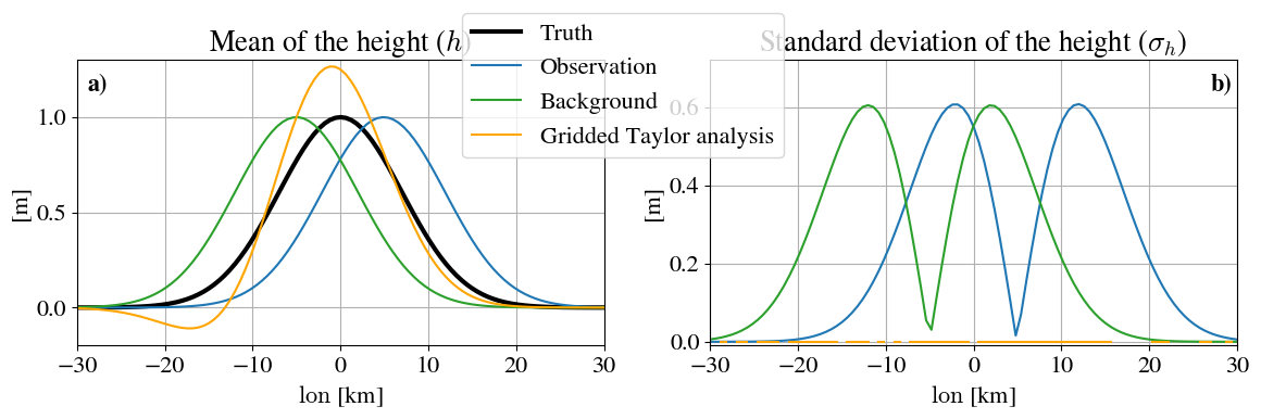
Figure A1 Taylor-linearized uncertainty propagation for the position-perturbation configuration (Experiment #2); see Fig. 3 for the corresponding ensemble-based propagation. (a) Background mean, observation mean, and the resulting Taylor-linearized BLUE analysis mean height: the Taylor-linearized BLUE analysis (orange) exhibits an unphysical negative undershoot on 28.7 % of grid points. (b) Taylor-propagated standard deviation of the background and observation (prior), and of the resulting analysis (posterior); note the vertical scale extends to twice the maximum of Fig. 3b, reflecting the larger peak values of the Taylor-propagated prior standard deviations. The prior curves drop to zero with a slope discontinuity at their respective peaks ($p=-\mathrm{5}$ and $p=+\mathrm{5}$ km, where $\partial h/\partial p=\mathrm{0}$ by symmetry), while the posterior standard deviation collapses to numerically negligible values almost everywhere, reflecting the rank-deficiency of the underlying covariance matrices.

Figure A1 illustrates the Taylor-linearized propagation discussed in Sect. 2.1, for the position-perturbation configuration (Experiment #2); the corresponding ensemble-based (Monte Carlo) propagation for the same configuration is shown in Fig. 3 (Sect. 4.1) and is not repeated here. The pathology extends to the posterior covariance itself: because ${\mathbf{B}}_{\text{Taylor}}^{\text{grid}}$ and ${\mathbf{R}}_{\text{Taylor}}^{\text{grid}}$ are each rank-1 (only p is uncertain), their sum is at most rank 2, and the resulting posterior covariance collapses to numerically negligible values (diagonal entries of order 10⁻¹⁶–10⁻¹⁸, occasionally slightly negative due to floating-point cancellation in the near-singular pseudo-inverse) almost everywhere on the grid, a spuriously overconfident analysis, rather than merely a biased one.